Polarimetry as a Tool for Observing Orographic Gravity Waves on Venus

HAL Id: insu-03226091

https://hal-insu.archives-ouvertes.fr/insu-03226091

Submitted on 14 May 2021

HAL is a multi-disciplinary open access

archive for the deposit and dissemination of

sci-entific research documents, whether they are

pub-lished or not. The documents may come from

teaching and research institutions in France or

abroad, or from public or private research centers.

L’archive ouverte pluridisciplinaire HAL, est

destinée au dépôt et à la diffusion de documents

scientifiques de niveau recherche, publiés ou non,

émanant des établissements d’enseignement et de

recherche français ou étrangers, des laboratoires

publics ou privés.

Distributed under a Creative Commons Attribution - NonCommercial| 4.0 International

for Observing Orographic Gravity Waves on Venus. The Planetary Science Journal, IOP Science, 2021,

2, 96 (12p.). �10.3847/psj/abf4cf�. �insu-03226091�

Polarimetry as a Tool for Observing Orographic Gravity Waves on Venus

1

Faculty of Aerospace Engineering, Delft University of Technology, Delft, The Netherlands;G.Mahapatra@tudelft.nl

2

Department of Physics, Oxford University, Oxford, UK 3

CNRS/INSU, LATMOS-IPSL, Guyancourt, France 4

Laboratoire de Météorologie Dynamique(LMD/IPSL), Sorbonne Université, Centre National de la Recherche Scientifique, École Polytechnique, École Normale Supérieure, Paris, France

5_{Institut Universitaire de France, Paris, France}

Received 2020 May 26; revised 2021 March 16; accepted 2021 March 30; published 2021 May 13

Abstract

Planet-wide stationary gravity waves have been observed with the thermal camera on the Akatsuki spacecraft. These waves have been attributed to the underlying surface topography and have successfully been reproduced using the Institut Pierre Simon Laplace(IPSL) Venus Mesoscale Model (VMM). Here, we use numerical radiative transfer computations of the total and polarized fluxes of the sunlight that is reflected by Venus under the conditions of these gravity waves to show that the waves could also be observed in polarimetric observations. To model the waves, we use the density perturbations computed by the IPSL VMM. We show the computed wave signatures in the polarization for nadir-viewing geometries observed by a spacecraft in orbit around Venus and as they could be observed using an Earth-based telescope. We find that the strength of the signatures of the atmospheric density waves in the degree of polarization of the reflected sunlight depends not only on the density variations themselves, but also on the wavelength and the cloud top altitude. Observations of such wave signatures on the dayside of the planet would give insight into the occurrence of the waves and possibly into the conditions that govern their onset and development. The computed change in degree of polarization due to these atmospheric density waves is about 1000 ppm at a wavelength of 300 nm. This signal is large enough for an accurate polarimeter to detect.

Unified Astronomy Thesaurus concepts: Venus(1763);Polarimetry (1278);Radiative transfer (1335); Planetary atmospheres(1244)

1. Introduction

Gravity waves are thought to play a key role in the transfer of energy and momentum from the lower to the upper parts of the Venus atmosphere, and through this would influence the super-rotation in the atmosphere(Hou & Farrell1987; Peralta et al.2008). Multiple and different types of observations have

shown that the upper atmosphere of Venus carries various types of gravity waves (Kasprzak et al. 1988; Piccialli et al.

2014; Peralta et al. 2017). Some wave patterns were found in

images of the clouds (Markiewicz et al. 2007; Peralta et al.

2008, 2020; Piccialli et al. 2014), and others revealed their

presence through the variations they leave in the local temperatures. In particular, the JAXA Akatsuki spacecraft’s Longwave Infrared Camera observed huge waves covering the planet almost from the southern to the northern poles(Fukuhara et al. 2017) on 2015 December 7, just five hours after the

spacecraft’s orbital insertion. These waves and the associated local density variations are what we focus on in this paper.

First in situ measurements of variations in the local temperatures and wind profiles that were attributed to atmo-spheric waves were made by the Pioneer Venus orbiter (Seiff et al. 1985). In particular, the Orbiter Neutral Mass

Spectro-meter(ONMS) measured variations in gas density in the upper atmosphere(Kasprzak et al.1988), and during the aerodynamic

drag experiments that were performed in the last orbits of

ESA’s Venus Express mission, wave-like perturbations were detected in the thermosphere(Müller-Wodarg et al.2016).

Small-scale(<100 km) waves in the Venus atmosphere have been studied with a turbulence-resolving numerical model that included a convective layer within the clouds(Imamura et al.

2014; Lefèvre et al.2018,2017). The formation of this

planet-wide wave observed by the Akatsuki spacecraft was attributed to the underlying mountainous Aphrodite Terra region (Fukuhara et al. 2017; Kouyama et al. 2017b; Lefèvre et al.

2020), see Figure1. Anomalies at the cloud tops that appeared to be associated with mountain waves were observed above the Beta Regio area with the IR2 instrument(2.02 μm wavelength, Satoh et al.2017) and above Aphrodite Terra, Atla, and Beta

Regio with the UV imager on the Akatsuki spacecraft(Kitahara et al. 2019). Indeed, stationary waves above the main

topographical features on the southern hemisphere of Venus were also detected by VIRTIS on the Venus Express mission (Peralta et al.2017).

The mountain waves’ dynamics was studied using limited-area mesoscale numerical modeling by Lefèvre et al. (2020). The

modeling shows that these waves are generated by the interaction between the windflow and the topography, with a peak of activity in the late afternoon controlled by the atmospheric stability. The waves propagate vertically to the cloud tops. At the cloud tops, the waves can perturb the local cloud altitudes by as much as 600 m and the local temperatures by± 2 K. Temperature anomalies larger than 0.5 K can remain present for about 10 Earth days (Kouyama et al.2017a; Lefèvre et al.2020). The waves transport

upward heat and momentum that affect the circulation and even the length of the Venus day, as was demonstrated by global climate modeling(Navarro et al.2018). It is clear that observing

© 2021. The Author(s). Published by the American Astronomical Society.

Original content from this work may be used under the terms of theCreative Commons Attribution 4.0 licence. Any further distribution of this work must maintain attribution to the author(s) and the title of the work, journal citation and DOI.

and characterizing these waves is crucial for a better under-standing of the current Venus atmosphere as well as its evolution. In this paper, we study the use of reflected sunlight, and in particular, polarimetry, i.e., the measurement of the state of polarization of light, for the detection and characterization of these gravity waves. Polarimetry has been successfully used to determine the Venus cloud particle refractive index, size distribution, cloud top altitude, and the nature of overlying haze particles (Hansen & Hovenier 1974; Kawabata et al. 1980; Knibbe et al.1995; Braak et al.2002; Rossi et al.2015). The state

of polarization of this light is sensitive to the optical properties of the particles that scatter the light, the scattering angle, and the number of times that the light is scattered. In particular, light that has been scattered by gaseous molecules can have a high degree of(linear) polarization (Hansen & Travis1974), depending on the

scattering angle. Because the gravity waves such as those observed by the Akatsuki spacecraft (Fukuhara et al.2017) are

in essence density variations in the atmospheric gas(Lefèvre et al.

2020), these waves are expected to cause a variation in the state

of polarization of the reflected light. We present results of computations of the total and polarized fluxes and the degree of polarization of the sunlight that is reflected by Venus in the presence of these gravity waves as computed with the Venus Mesoscale Model(VMM; Lefèvre et al.2020).

The outline of this paper is as follows. In Section 2 we describe our numerical method, including the properties of our model atmosphere and our use of the numerical results of the VMM, i.e., the local atmospheric density variations due to the gravity waves. In Section 3 we present and discuss our numerical results. Section4finally contains a summary and our

conclusions.

2. Description of the Numerical Method 2.1. Definitions of Fluxes and Polarization

Our aim is to compute the total and linearly polarizedfluxes of sunlight that is reflected by Venus when gravity waves travel

through its atmosphere. We describe the total and polarized fluxes of light with the following Stokes (column) vector F (see Hansen & Travis1974):

[ ] ( )

=

F F Q U V, , , , 1 with F the totalflux, Q and U the linearly polarized fluxes, and V the circularly polarized flux. In general, the Stokes vector elements depend on the wavelengthλ. Element V of sunlight that is reflected by Venus is very small and varies within a few dozen parts per million (ppm) depending on the atmosphere and observation geometry (Kemp et al. 1971; Kawata 1978; Rossi & Stam2018).

We assume that the sunlight that is incident on Venus is unidirectional and unpolarized (e.g., Kemp et al.1987), such

thatF0= F0[1, 0, 0, 0] = F01, withπF0the total incident solar flux measured perpendicularly to the direction of propagation of the light. Thus the reflected fluxes shown here are normalized fluxes and the actual values can be obtained in a straightforward manner by scaling them to the actual value of incoming sunlight in W m−2on Venus.

The linearly polarized fluxes Q and U of the reflected sunlight are defined with respect to a reference plane. We perform our model calculations for local reflected light with a nadir-viewing direction and a few solar zenith angles, as could be observed by a spacecraft orbiting Venus, and for a distant view, as would be observable with an Earth-based telescope. In our computations of locally reflected light, the reference plane is the local meridian plane, i.e., the vertical plane containing the local zenith direction and the direction to the observer. In our computations of light reflected by Venus as a whole as observable with an Earth-based telescope, the reference plane is the planetary scattering plane, i.e., the plane containing the centers of the Sun, Venus, and the Earth.

The degree of(linear) polarization of the reflected light is in general defined as the ratio of (linearly) polarized fluxes to the

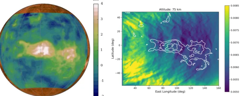
Figure 1.Elevation(in km) of the Aphrodite Terra region mapped on the Venus sphere (on the left), and the corresponding computed pressure map (in atm) at an altitude of 75 km, with Aphrodite Terra outlined in white(on the right). The pressure contours have been derived from isopotential temperature surface fields (Lefèvre et al.2020). The covered area (on the right) spans 108° in latitude and 144° in longitude. The orographic wave peaks above the Aphrodite Terra pressure map (on the

totalflux, as follows:

( )

= +

P Q2 U2 F. 2

For the results with the local viewing geometry, however, the illumination and viewing geometries in combination with our choice of reference plane are such that the linearly polarizedflux U is always zero. We therefore use a definition of the degree of polarization that includes information about the direction of polarization in this case,

( ) =

-PS Q F. 3

If PS> 0 (PS< 0), the light is polarized perpendicular (parallel) to the reference plane.

2.2. Optical Properties of the Model Atmosphere The model atmosphere of Venus is composed of a stack of 71 horizontally homogeneous layers that contain gas and, optionally, cloud or haze particles. The optical properties of each of the layers are described by the layer’s optical thickness b, the single-scattering albedo, and the single-scattering matrix S of the particles in the layer. The atmosphere is bounded below by a horizontally homogeneous surface, which we assume to be black(because of the high optical thickness of the clouds, the actual value of the surface albedo is irrelevant).

The total optical thickness b of an atmospheric layer at wavelengthλ is given by the sum of the layer’s gaseous optical thickness, bm, and the layer’s aerosol (i.e., cloud or haze) optical thickness, ba, as follows:

( )l = ( )l + ( )l ( )

b bm ba . 4

The layers of our model atmosphere all contain pure carbon-dioxide(CO2) gas. For our radiative transfer computations, we use wavelengths where CO2 does not have any significant absorption; the single-scattering albedo of the gas is thus 1.0. The gas optical thickness, bm, of an atmospheric layer is computed as

( )l = s l( ) ( )

bm Nm m , 5

with Nmthe layer’s gaseous column number density (in m−2), and σm the scattering cross-section of the gas molecules (in m2), which is given by (see, e.g., Stam et al.1999)

( ) ( ( ) ) ( ( ) ) ( ) ( ) ( ) s l p l l l d l d l = -+ + -N n n 24 1 1 2 6 3 6 7 , 6 m 3 L2 4 2 2 2 2

with NL Loschmidt’s number, n the refractive index of CO2 under standard conditions, and δ the depolarization factor of CO2. For both n and δ, we use the wavelength-dependent values of Sneep & Ubachs (2005). Under assumption of

hydrostatic equilibrium, a layer’s gas column number density Nmis computed according to ( ) = -N N p p mg , 7 m A bot top

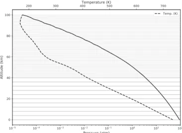
with NAAvogadro’s number, pbotand ptopthe pressures at the bottom and top of the atmospheric layer, respectively, m the average molar mass of the gas, i.e., 44.01 g mol−1for CO2, and g the acceleration of gravity, which we assume to be altitude independent and equal to 8.87 m s−2. Figure2shows the standard (i.e., unperturbed by a gravity wave) pressure and temper-ature profiles across our model atmosphere (Seiff et al. 1985)

and the geometrical thickness of the atmospheric layers. Note that the total and polarizedfluxes of the light that is reflected by Venus are virtually insensitive to the atmospheric composi-tion and density below the main cloud deck, thus below 40–50 km.

The gravity waves cause variations in the local atmospheric pressure, and hence in the local gas density and the gas optical thickness bmof the atmospheric layers through which the wave travels. We compute the local variations in bm of the whole range (0–100 km) of the atmosphere using the local pressure variations resulting from the gravity wave model computations described by Lefèvre et al.(2020). They used the Institut Pierre

Simon Laplace(IPSL) VMM to simulate the orographic wave that was observed 15° west of the Aphrodite Terra region of Venus by the Akatsuki spacecraft (Fukuhara et al. 2017; Kouyama et al.2017b).

In the VMM, the nonhydrostatic WRF dynamical core (Skamarock & Klemp 2008) is coupled with the radiative

transfer code of the IPSL Venus General Circulation Model (GCM; Lebonnois et al.2015) to compute the solar heating and

the thermal radiationfield of the atmosphere. Furthermore, the latitudinal varying cloud model of Haus et al.(2014,2015) is

implemented. The initial and horizontal boundary conditions are determined by the GCM(Garate-Lopez & Lebonnois2018),

which is updated every 1/100 Venus day, thus about every 28 Earth hours. Lefèvre et al.(2020) computed the wave over

Aphrodite Terre with a spatial resolution of 40× 40 km2and 300 levels in the vertical direction.

Lefèvre et al.(2020) found that the isopotential temperature

can be used as a tracer for the deformation of the cloud top by waves. Thus, by choosing one value for the isopotential temperature, corresponding temperature and pressure maps can be reconstructed. We use the pressure values corresponding to isopotential temperature maps over Aphrodite Terra in the radiative transfer computations. Figure 1 illustrates the local pressure variations with isopotential temperature due to the wave over the Aphrodite Terra region at an altitude of 75 km. Note that at low altitudes, the pressure variations follow the topography of the underlying Aphrodite Terra area, and at higher altitudes, such as at 75 km, the variations are due to the orographic waves. Figure3shows the map of bm, as perturbed

Figure 2.Vertical profiles of the pressure (solid line) and the temperature (dashed line) across our unperturbed Venus model atmosphere (Seiff et al.1985). The horizontal lines indicate the geometrical thicknesses of the

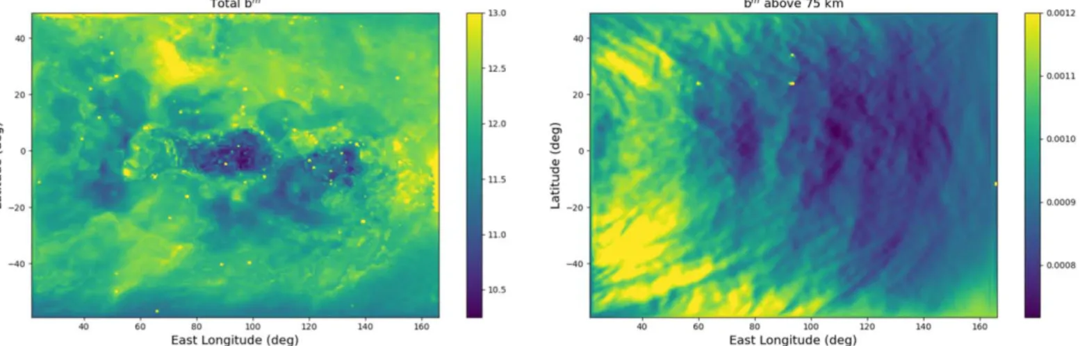
due to the gravity wave over the Aphrodite Terra region (see Figure 1), computed for the whole atmosphere and for the

atmosphere above 75 km. In the latter, the density wave is clearly visible. The maximum change in pressure from the wave perturbation occurs at 80° longitude.

Figure 4 shows our cloud and haze vertical profiles. The aerosol (i.e., cloud or haze) optical thickness ba has been adapted from in situ measurements by Knollenberg & Hunten (1980). For the cloud and haze, bais 30 and 0.1, respectively. In principle, these optical thicknesses depend (somewhat) on the wavelength, but we keep them constant for this invest-igation. Both the cloud and haze particle densities decrease exponentially with altitude with a scale height of 4 km (see Figure 4). We define the cloud top altitude as the altitude at

which the cloud optical thickness equals 1.0 measured from the top of the atmosphere (ignoring the haze).

The cloud and haze particles are assumed to be spherical, with their sizes described by a log-normal size distribution (Hansen & Travis1974) with a modal radius rgand a variance σ. Following Pollack et al. (1980) and Fedorova et al. (2016),

we use rg= 1.05 μm and σ = 1.21 for the cloud particles, and rg= 0.15 μm and σ = 1.91 for the haze particles, which is derived from the observations of cloud particle size-distribution by the LCPS instrument on board the Pioneer Venus mission

(Knollenberg & Hunten1980). For the refractive index of both

the cloud and haze particles, we use values that are wavelength dependent and representative for 75% sulphuric acid solution (Palmer & Williams1975). We compute the optical properties

of the cloud and haze particles, i.e., their scattering cross-section and single-scattering matrix, using the Mie-algorithm as described by De Rooij & Van der Stap(1984). To account for

the absorption by the cloud and haze particles atλ = 300 nm, we take a nonzero value for the imaginary part of the refractive index, ni= 0.0007, which yields a planet spherical albedo of 0.4 (Pollack et al. 1980). The planet spherical albedo was

accounted for using the similarity relation described in Hansen & Hovenier (1974), which was also applied by Bailey et al.

(2018) for their polarized flux computations of Venus. At

λ = 600 and 900 nm, the imaginary part of the refractive index equals zero, and the single-scattering albedo of the cloud and haze particles is thus one. At 300 nm, the single-scattering albedo of the cloud and haze particles is ∼0.972. Figure 5

shows the phase function(i.e., the scattered flux) and degree of polarization of incident unpolarized light that is singly scattered by the cloud and haze particles at the wavelengths of our interest.

The single-scattering matrix of the scatterers in the layer is computed using ( ) ( ) ( ) ( ) ( ) ( ) ( ) l l l l l l = + S b S b S b , 8 m m sca a a

with Smthe single-scattering matrix of the gas, for which we use the anisotropic Rayleigh scattering matrix as described by Hansen & Travis(1974), and Sathe single-scattering matrix of the aerosol, i.e., the cloud or haze particles. b_scaa ( )l is the wavelength-dependent aerosol scattering optical thickness.

2.3. The Radiative Transfer Algorithm

The reflected flux vector F (Equation (1)) strongly depends

on the illumination and viewing geometries, in addition to the optical properties of the model atmosphere. These geometries are defined with the following angles: θ0is the angle between the local zenith and the direction to the Sun, θ is the angle between the local zenith and the direction to the observer, and f is the azimuthal angle between the direction of propagation of the incident light and the direction toward the observer. Because our plane-parallel model atmosphere is rotationally

Figure 3.Left: the total gas optical thickness bmof the Venus atmosphere. Right: the gas optical thickness of the atmosphere above 75 km. These optical thicknesses pertain toλ = 600 nm, and have been calculated for an afternoon pressure map of the Aphrodite Terra region (Lefèvre et al.2020), as shown in Figure1.

Figure 4.Sample vertical distribution of the cloud and haze particles. Both the cloud and the haze have a scale height H of 4 km. The (wavelength-independent) optical thicknesses of the cloud and the haze are 30 and 0.1, respectively.

symmetric around the local vertical, only the difference between the azimuthal directions of the incident and the reflected light (f − f0) is relevant.

We use an efficient adding-doubling algorithm (de Haan et al.1987) to compute the light that is reflected by Venus. The

algorithm fully accounts for polarization in all orders of scattering. We used the PyMieDAP code (Rossi et al. 2018),

which is an open-source version of the adding-doubling algorithm. For our computations of locally reflected light, we use a nadir-viewing geometry, thus with θ = 0°, and vary θ0 between 0° and 90° (f − f0is thus undefined and set equal to 0°). For our computations for Earth-based Venus observations, we use the planetary phase angleα, measured between the Sun and the Earth from the center of Venus (0° „ α „ 180°), to describe the illumination and viewing geometries of the planet. We use 80 Gaussian quadrature points for interpolating between subgrid geometries in all of our computations.

3. Results

3.1. Sensitivity of F, Q, and PSto the Total Gas Optical Thickness

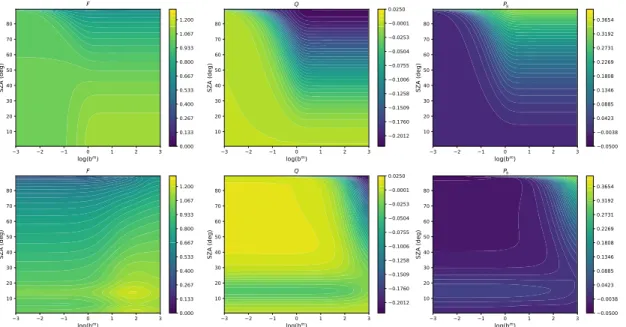
Before discussing the signatures of gas density variations due to gravity waves in reflected sunlight, we discuss how the total and polarizedfluxes F and Q and the degree of polarization PSdepend on the gas optical thickness bm. The top row in Figure6shows the dependence of F, Q, and PS on bmabove a white, Lambertian reflecting surface. We use this surface instead of an aerosol layer to avoid introducing angular effects due to the scattering of light by the cloud and haze particles. These effects have been included in the bottom row of Figure6, where a thick cloud layer replaces the white surface. The solar zenith angleθ0ranges from 0° and 90°, and the viewing zenith angle θ is zero (nadir view, thus U equals zero). Note that bm above 65 km in the unperturbed atmosphere is about 0.01 atλ = 600 nm.

Figure 6.Totalflux F (left column), linearly polarized flux Q (middle column), and degree of polarization PS(right column) as functions of the atmospheric gas

optical thickness bm_{and the solar zenith angleθ}

0. The viewing zenith angleθ is 0° (nadir view). In the top row, the atmosphere is cloud free and the surface reflects

Lambertian with an albedo of 1.0. In the bottom row, the atmosphere contains an additional optically thick cloud with its top at 65 km.

Figure 5.Phase function(left) and degree of polarization (right) of incident unpolarized light that is singly scattered by the cloud particles (solid colored lines), haze particles(dashed colored lines), and the gaseous molecules (solid black lines) at three wavelengths. Note that the wavelength dependence of the molecular scattering (through depolarization factor δ) is so small that we show only one line. All particles are distributed in size according to a log-normal distribution. The phase functions have been normalized such that averaged over all scattering directions, they equal 1.0(see Hansen & Travis1974).

Figure6shows that with a white surface instead of a cloud and forθ0Š 50°, the total flux F increases with increasing bm because of the increase in scattering in the atmosphere in combination with the short path-length through the atmosphere and the white surface. For larger θ0, F decreases with increasing bm both because the incident flux decreases (measured parallel to the atmosphere) and because the contribution of the surface reflection decreases. When bm is approximately larger than 10, F has reached its asymptotic value and is virtually constant for a given value ofθ0. Without a cloud, Q is negative for all θ0 and bm because the only scatterers are gas molecules. For small bm, Q is close to zero because of the unpolarized surface reflection. With increasing bm, |Q| increases due to the increased scattering by the gas, except for the lowest values of θ0, where the single-scattering PS is very small (see Figure 5). Like F, Q reaches an asymptotic value when bm‹ 10. The degree of polarization PS increases with bm, except for the smallest θ0, where P≈ 0 because|Q| ≈ 0.

With a thick cloud instead of a white surface(the bottom row of Figure6), F, Q, and PSare strongly influenced by scattering in the cloud, especially when bmandθ0are small. In particular, for 0.1Š bmŠ 1 and θ0‹ 20°, F, Q, and PS appear to be insensitive to bm because they are mostly determined by the scattering by the cloud particles. For higher values of bm, F, Q, and PStend to their values with the white surface instead of the cloud underneath the atmosphere. Whenθ0≈ 15°, F, Q, and PS all show the glory. This feature is also prominent in the single-scattering curves of the cloud particles(Figure5) and is thought

to be due to interference of EM waves that traveled across the surface of the spherical particles(for an in-depth discussion of

this optical feature, see Laven2005). The detection of the glory

has been well documented on Venus (see Hansen & Hovenier 1974; García Muñoz et al. 2014; Petrova et al.

2015; Rossi et al.2015; Satoh et al.2015; Lee et al.2017).

3.2. Sensitivity of F, Q, and PSto the Vertical Distribution of the Gas Optical Thickness

The amplitude of a density perturbation caused by an atmospheric gravity wave increases exponentially with altitude (Frits & Alexander 2003). We have performed a sensitivity

study of the influence of the altitude of a density variation on F, Q, and PS by increasing the gas density and hence the gas optical thickness of single atmospheric layers by 1% in 2 km thick layers between 60 and 90 km (above 90 km, the gas density is too low to leave any effect) and by computing the resulting F, Q, and PSof the reflected light. At 60 km (90 km), the unperturbed gas density is 0.47 kg m−3 (0.00114 kg m−3), and we thus increase it to 0.474 7 kg m−3 (0.00115 kg m−3). The viewing angleθ is 0°, like before.

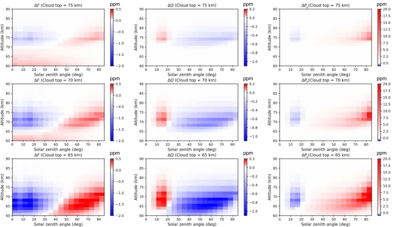
Figure7shows the relative differences in F, Q, and PSdue to the 1% gas density increases in single atmospheric layers for three different cloud top altitudes. It can be seen that a density increase in the lower atmospheric layers generally has a larger influence on F, Q, and PS, when the cloud top is lower. The reason is that with a lower cloud top altitude, the upper atmospheric layers contain fewer cloud particles, and the contribution of scattering by gas molecules is larger. When θ0Š 40°, increasing the density decreases F of the reflected light (at θ = 0°), except when the cloud top is high and the density increase is in the lower atmospheric layers(the top row

Figure 7.ΔF (left column), ΔQ (middle column), and ΔPS(right column; all in ppm) upon increasing the gas density or bscam in an atmospheric layer by 1 % as functions ofθ0for different cloud top altitudes: 75 km(top row), 70 km (middle row), and 65 km (bottom row). The cloud and haze scale heights are 4 km. The

wavelength is 600 nm, and the viewing angleθ = 0°. A positive/red (negative/blue) color indicates an increase (decrease) in F, Q, or PSwith an increase in b m

of Figure 7). The polarized flux Q increases with increasing

density when θ0 is smaller than about 25° (except when θ0≈ 0°, where Q is virtually zero), and Q decreases with

increasing density when θ0‹ 25°. The degree of polarization PSdecreases where Q increases. The change in PSis largest for the highest values ofθ0.

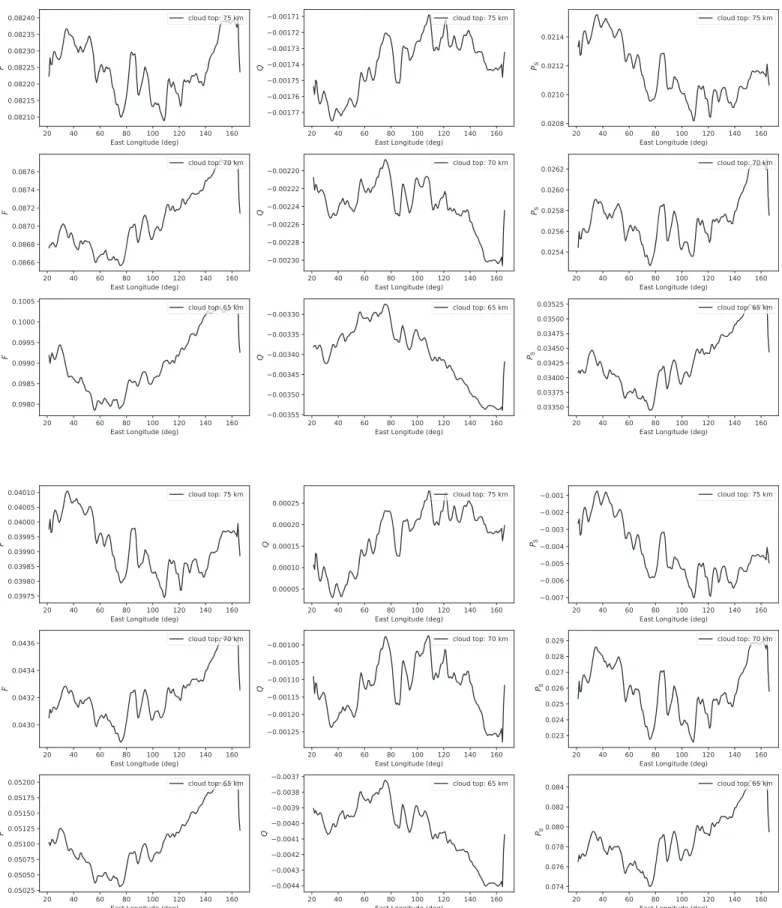
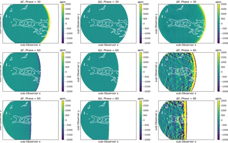
Figure 8. F(left column), Q (middle column), and PS(right column) at λ = 300 nm across the afternoon pressure map of Aphrodite Terra at a latitude of 0° for cloud

top altitudes of 75 km(top row), 70 km (middle row), and 65 km (bottom row). The viewing zenith angle θ is 0° (nadir view). For the top three rows, the solar zenith angleθ0= 30°, and for the bottom three rows, the solar zenith angle θ0= 60°. The maximum intensity of the wave occurs around 80° longitude.

3.3. F, Q, and PSAcross Aphrodite Terra

Here we present F, Q, and PS of the reflected sunlight as computed across Aphrodite Terra, using the density waves shown in Figure3. Figure8 shows longitudinal cross-sections pertaining to the latitude 0° for θ0= 30° and 60°, respectively, and for cloud top altitudes of 75, 70, and 65 km. The viewing zenith angle θ is, as before, 0°. As can be seen, for a given cloud top altitude andθ0, the patterns of F and Q, and PSare not correlated with wave structure across the latitude. This is due to the altitude dependence of the sensitivity of F and Q to density variations (see Figure 7). In particular, F shows

smaller-scale wave features than Q and PS, which are caused by the horizontal altitude variations of the underlying surface(see Figure10). The pattern of PSappears to be the inverse of that of Q, which is a consequence of the negative sign introduced in Equation (3). We recall that positive PS denotes polarization perpendicular to the reference plane. Changing the cloud top altitude changes F, but not the general pattern variation with longitude. The influence of the cloud top altitude is stronger on Q than on F: the overall shape of the curves changes significantly with changing cloud top altitude, and while some peaks and dips appear to be relatively insensitive to the cloud top altitude, their strengths with respect to other features change. The anticorrelation of F and Q increases with decreasing cloud top altitude caused by the reflected light from density waves deeper in the atmosphere. The PScurves behave similarly to those of Q.

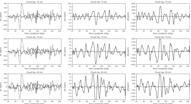
In Figure9the background continuum of theθ0= 60° curves in Figure8has been removed to better show the variations. For each data point, the background continuum was computed by averaging the 12 surrounding data points, or equivalently, across 4°.2 of longitude. In addition to the curves for 300 nm,

we have added those for wavelengths of 600 and 900 nm. It can be seen that the variations in Q and PSare largest at 300 nm and smallest at 900 nm. This is due to the 1/λ4dependence of the Rayleigh scattering cross-section, see Equation (6) and

Figure 6: with increasing λ for a given gas density, b_scam decreases, and hence|Q| and PSdecrease. For F, the variations are largest at 600 nm and smallest at 300 nm. This is due to an interplay between the scattering by gas (F decreases with increasingλ), clouds (F increases with increasing λ), and the observational geometry. Figure9also shows that the variations in Q and PS increase with decreasing cloud top altitude (see Figure7). In particular, the variations in PSare on the order of 100 ppm for the highest clouds shown here, and a few times larger for the lowest clouds. The variations in F appear to be independent of the cloud top altitude.

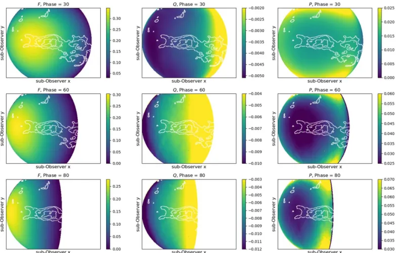
Figure10 shows F, Q, and PS across the Aphrodite Terra region for three values of θ0. Here, λ = 300 nm, where the variations in Q and PSare largest(see Figure9), and the cloud top is at 65 km. The maps of F for the different θ0 show different patterns: in particular, with increasingθ0, the surface features become less apparent as the scattering in the atmosphere increases. The patterns across the maps of Q show hardly any dependence on θ0, except for the absolute values: with increasing θ0, the single-scattering angle increases, and |Q| of the light scattered by the gas molecules increases (see Figure5). The maps of Q also reveal the wave pattern clearer

than F, while the underlying topography is indistinguishable because Q originates from higher altitudes than F. The maps of PS are similar to those of Q. As we have seen before in Figure9, the strength of the variations in Q and PSincreases withθ0. Figure11shows PSatθ0= 60° from Figure10with the background signal removed. We used two different

Figure 9.Similar to Figure8, but the background is subtracted(for each data point, the background is the average of the 12 surrounding data points), and for 300 nm (solid lines, see Figure8), 600 nm (dashed lines), and 900 nm (dotted lines). The solar zenith angle θ0is 60° and the viewing angle θ = 0°. The values are shown

Gaussian background removal filters: a high-pass filter and a low-passfilter. The high-pass filter has a σ = 15 and low-pass filter has. σ = 3. The choice of filter affects the substructure in the wave pattern in PS, but does not change the absolute change in PS.

Figures 7–11 showed the reflected light signals for a local viewing geometry with the local viewing angle fixed to nadir view (θ = 0) and a constant solar zenith angle. We use a

constant viewing geometry in each map so as to determine the contribution of the signal due to the waves. Figure 12shows the signals as they would be observable from Earth(e.g., from an Earth-orbiting telescope or from the ground) for three planetary phase angles α. Here, the local solar zenith and viewing angles thus depend on the location on the planetary disk. Please note that here we add the contribution of U(which is generally nonzero for the planet-wide view) in calculating

Figure 11.Map of the change in PSfrom Figure10forθ0= 60° with two different filters applied to remove the background signal: a high-pass filter with σ = 15 (left)

and a low-passfilter with σ = 3 (right). The values are shown in ppm. The maximum change in PSin the low-passfilter (right) is 2000 ppm at around 80° east

longitude.

Figure 10. F(first column), Q (second column), and PS(third column; all in ppm) across Aphrodite Terra. The cloud top is at 65 km, and the wavelength λ is 300 nm.

our degree of polarization P and thus use the formula in Equation (2). Figure 13 is similar to Figure 12, but the background is removed with a Gaussianfilter with σ = 3. Note that these computations do not include turbulence in the Earth’s atmosphere, which would decrease the spatial resolution when observing the planet with a ground-based telescope.

In Figure 12hardly any wave-like patterns are visible. The main variations in F, Q, and P are smooth and due to the variation of the illumination and viewing angles across the disk. In Figure13Q and especially P do show patterns due to the density variations of the gravity wave. The pattern strength increases with increasing α, as the average θ0, across the planetary disk increases and the average single-scattering angle thus decreases (see Figure10).

4. Summary and Conclusions

We have used pressure variations due to atmospheric gravity waves as computed by the VMM(Lefèvre et al.2020), which

successfully simulated waves over the Venus Aphrodite Terra region as observed at IR wavelengths by the JAXA Akatsuki spacecraft (Fukuhara et al. 2017; Kouyama et al. 2017b) to

investigate the use of reflected sunlight observations for the detection of such waves. Waves in the upper tenuous part of the Venus atmosphere (∼70 km) will escape methods such as IR observations, which were successful in detecting waves in the lower, denser parts of the Venus atmosphere. Observations of reflected sunlight will also allow detecting the waves on the

dayside of Venus, which would help understanding the atmospheric conditions that trigger their appearance.

Our numerical simulations indicate that the (linearly) polarizedflux and the degree of polarization P of sunlight that is reflected by Venus are indeed sensitive to variations in the gas density, and through this, to variations of the gas optical thickness bmabove the Venusian clouds, while the totalflux F is more sensitive to the properties of the clouds themselves. The polarized flux increases with increasing atmospheric gas density above the clouds as more light is scattered by gas molecules, except for geometries where the light that has been singly scattered has a very low degree of polarization, such as when the Sun is overhead for a nadir-looking instrument on a spacecraft orbiting or flying past Venus. The degree of polarization P of the reflected sunlight shows a similar behavior as the polarized flux: P increases with increasing gas optical thickness bm, except in the back-scattering direction because there the single-scattering P equals zero.

For a nadir-viewing mode, the variations in F, Q(U equals zero in our geometries), and PSincrease with increasing solar zenith angle as the gas density along the optical path increases. Varying the vertical location of the gas density variations shows that F appears to be slightly more sensitive to waves in deeper atmospheric layers than Q and PS.

The variations in F, Q, and PS decrease with increasing wavelength. This is not surprising because the Rayleigh scattering cross-section of the gaseous molecules also decreases with increasing wavelength. At 300 nm, variations in F are in the order of a few 100 ppm, in|Q| in the order of 50 ppm, and

Figure 12.Similar to Figure10, except for an Earth-based observer line of sight for three planetary phase anglesα: 30° (top row), 60° (middle row), and 80° (bottom row). Only the illuminated and observable part of the planetary disk is shown.

in PS in the order of 500 ppm. The variations in Q and PSat 300 nm are a factor of about 10 stronger than at 600 nm and a factor of about 100 stronger than at 900 nm. In F, the variations at 300 nm are about twice as strong as those at 600 nm and about four times as strong as those at 900 nm. Observations at shorter wavelengths would thus be better suited for detecting these waves.

For our simulations, we assumed a constant cloud top altitude across each scene on the planet. In reality, the Venusian clouds show spatial variability(Sato et al.2020; Fedorova et al.

2016): the average cloud top altitudes decrease with increasing

latitude, ranging between 75 to 65 km. Our results show that the strength of the wave variations in the polarized flux and degree of polarization increases with decreasing cloud top altitude (see Figure 9). If the cloud top altitude were to vary

across an observed scene, the strength of the observed variations would thus also depend on the variations in the cloud top altitude. Distinguishing the variations due to gas density variations from those due to cloud top variations would be possible when the density wave moves with respect to the underlying clouds because the typical wind speeds range from 100 to 350 km h−1near the cloud tops(Sánchez-Lavega et al.

2017; Garate-Lopez & Lebonnois 2018; Horinouchi et al.

2018).

We based our analysis of orographic gravity waves over the Aphrodite Terra region as observed by Akatsuki (Fukuhara et al. 2017; Kouyama et al. 2017b) and modeled by Lefèvre

et al.(2020). The scope of our analysis extends to gas density

variations due to other types of atmospheric waves. For example, the Pioneer Venus ONMS instrument observed

wave-like density fluctuations in the Venus thermosphere that were linked to the vertical propagation of inertial gravity waves (Kasprzak et al.1988). The Venus Express Aerobreaking Drag

Experiment registered local density perturbations (Müller-Wodarg et al. 2016) in the uppermost atmosphere of Venus

in an altitude region of 130–200 km. Although the density variations would be too small to yield measurable signal variations(see Figure7) at these high altitudes, polarimetry that

is sensitive to upper atmospheric variations might be a powerful tool for detecting them in the future and for providing more information about them.

Our computations offlux and polarization signals across the disk of Venus due to the waves at different planetary phase angles (Figure 13) show variations in P on the order of

100 ppm at intermediate to large phase angles (60°–80° in Figure 13). Such variations are achievable with modern-day

polarimeters on Earth-based telescopes even though Earth’s atmosphere introduces some spatial blurring. One such example of a highly sensitive instrument is the experimental ExPo instrument, which had a polarimetric signal sensitivity better than 100 ppm(Rodenhuis et al.2008).

Of course, Venus is not the only planet with gravity waves traveling through its atmosphere. Many detections of such waves in the Earth’s atmosphere have been reported (Gong et al.2015; Chou et al.2017), and high-precision polarimetry

from an Earth-orbiting satellite could help to further character-ize such waves on the dayside.

Funding support for G.M. was provided by NWO, the Netherlands Organization for Scientific Research. M.L.

Aymeric Spiga https://orcid.org/0000-0002-6776-6268

Daphne M. Stam https://orcid.org/0000-0003-3697-2971

References

Bailey, J., Kedziora-Chudczer, L., & Bott, K. 2018,MNRAS,480, 1613

Braak, C., de Haan, J., Hovenier, J., & Travis, L. 2002,JGRE,107, 5029

Chou, M. Y., Lin, C. C., Yue, J., et al. 2017,GeoRL,44, 1219

de Haan, J. F., Bosma, P., & Hovenier, J. 1987, A&A,183, 371

De Rooij, W., & Van der Stap, C. 1984, A&A,131, 237

Fedorova, A., Marcq, E., Luginin, M., et al. 2016,Icar,275, 143

Frits, D. C., & Alexander, M. J. 2003,RvGeo,41, 1003

Fukuhara, T., Futaguchi, M., Hashimoto, G. L., et al. 2017,NatGe,10, 85

Garate-Lopez, I., & Lebonnois, S. 2018,Icar,314, 1

García Muñoz, A., Pérez-Hoyos, S., & Sánchez-Lavega, A. 2014, A&A,

566, L1

Gong, J., Yue, J., & Wu, D. L. 2015,JGRD,120, 2210

Hansen, J. E., & Hovenier, J. 1974,JAtS,31, 1137

Hansen, J. E., & Travis, L. D. 1974,SSRv,16, 527

Haus, R., Kappel, D., & Arnold, G. 2014,Icar,232, 232

Haus, R., Kappel, D., & Arnold, G. 2015,P&SS,117, 262

Horinouchi, T., Kouyama, T., Lee, Y. J., et al. 2018,EP&S,70, 10

Hou, A. Y., & Farrell, B. F. 1987,JAtS,44, 1049

Imamura, T., Higuchi, T., Maejima, Y., et al. 2014,Icar,228, 181

Markiewicz, W., Titov, D., Limaye, S., et al. 2007,Natur,450, 633

Müller-Wodarg, I. C., Bruinsma, S., Marty, J.-C., & Svedhem, H. 2016,NatPh,

12, 767

Navarro, T., Schubert, G., & Lebonnois, S. 2018,NatGe,11, 487

Palmer, K. F., & Williams, D. 1975,ApOpt,14, 208

Peralta, J., Hueso, R., Sánchez-Lavega, A., et al. 2008,JGRE,113, E00B18

Peralta, J., Hueso, R., Sánchez-Lavega, A., et al. 2017,NatAs,1, 0187

Peralta, J., Navarro, T., Vun, C., et al. 2020,GeoRL,47, e87221

Petrova, E. V., Shalygina, O. S., & Markiewicz, W. J. 2015,P&SS,113, 120

Piccialli, A., Titov, D. V., Sanchez-Lavega, A., et al. 2014,Icar,227, 94

Pollack, J. B., Toon, O. B., Whitten, R. C., et al. 1980,JGR,85, 8141

Rodenhuis, M., Canovas, H., Jeffers, S., & Keller, C. 2008, Proc. SPIE,

7014, 70146T

Rossi, L., Berzosa-Molina, J., & Stam, D. M. 2018,A&A,616, A147

Rossi, L., Marcq, E., Montmessin, F., et al. 2015,P&SS,113, 159

Rossi, L., & Stam, D. M. 2018,A&A,616, A117

Sánchez-Lavega, A., Lebonnois, S., Imamura, T., Read, P., & Luz, D. 2017,

SSRv,212, 1541

Sato, T., Satoh, T., Sagawa, H., et al. 2020,Icar,345, 113682

Satoh, T., Ohtsuki, S., Iwagami, N., et al. 2015,Icar,248, 213

Satoh, T., Sato, T. M., Nakamura, M., et al. 2017,EP&S,69, 154

Seiff, A., Schofield, J., Kliore, A., et al. 1985,AdSpR,5, 3

Skamarock, W. C., & Klemp, J. B. 2008,JCoPh,227, 3465

Sneep, M., & Ubachs, W. 2005,JQSRT,92, 293