HAL Id: hal-02955490
https://hal.archives-ouvertes.fr/hal-02955490
Submitted on 1 Oct 2020
HAL is a multi-disciplinary open access
archive for the deposit and dissemination of
sci-entific research documents, whether they are
pub-lished or not. The documents may come from
teaching and research institutions in France or
abroad, or from public or private research centers.
L’archive ouverte pluridisciplinaire HAL, est
destinée au dépôt et à la diffusion de documents
scientifiques de niveau recherche, publiés ou non,
émanant des établissements d’enseignement et de
recherche français ou étrangers, des laboratoires
publics ou privés.
supernovae
Luc Dessart, D. John Hillier
To cite this version:
Luc Dessart, D. John Hillier. Radiative-transfer modeling of nebular-phase type II supernovae:
Depen-dencies on progenitor and explosion properties. Astronomy and Astrophysics - A&A, EDP Sciences,
2020, 642, pp.A33. �10.1051/0004-6361/202038148�. �hal-02955490�
Astronomy
&
Astrophysics
https://doi.org/10.1051/0004-6361/202038148© L. Dessart and D. J. Hillier 2020
Radiative-transfer modeling of nebular-phase type II supernovae
Dependencies on progenitor and explosion properties
Luc Dessart
1and D. John Hillier
21Institut d’Astrophysique de Paris, CNRS-Sorbonne Université, 98 bis boulevard Arago, 75014 Paris, France
e-mail: [email protected]
2 Department of Physics and Astronomy & Pittsburgh Particle Physics, Astrophysics, and Cosmology Center (PITT PACC),
University of Pittsburgh, 3941 O’Hara Street, Pittsburgh, PA 15260, USA Received 11 April 2020 / Accepted 3 July 2020
ABSTRACT
Nebular phase spectra of core-collapse supernovae (SNe) provide critical and unique information on the progenitor massive star and its explosion. We present a set of one-dimensional steady-state non-local thermodynamic equilibrium radiative transfer calculations of type II SNe at 300 d after explosion. Guided by the results obtained from a large set of stellar evolution simulations, we craft ejecta models for type II SNe from the explosion of a 12, 15, 20, and 25 M star. The ejecta density structure and kinetic energy, the56Ni mass,
and the level of chemical mixing are parametrized. Our model spectra are sensitive to the adopted line Doppler width, a phenomenon we associate with the overlap of FeIIand OIlines with Ly α and Ly β. Our spectra show a strong sensitivity to56Ni mixing since it determines where decay power is absorbed. Even at 300 d after explosion, the H-rich layers reprocess the radiation from the inner metal rich layers. In a given progenitor model, variations in56Ni mass and distribution impact the ejecta ionization, which can modulate the
strength of all lines. Such ionization shifts can quench CaIIline emission. In our set of models, the [OI] λλ 6300, 6364 doublet strength is the most robust signature of progenitor mass. However, we emphasize that convective shell merging in the progenitor massive star interior can pollute the O-rich shell with Ca, which would weaken the OIdoublet flux in the resulting nebular SN II spectrum. This process may occur in nature, with a greater occurrence in higher mass progenitors, and this may explain in part the preponderance of progenitor masses below 17 M that are inferred from nebular spectra.
Key words. radiative transfer – line: formation – supernovae: general
1. Introduction
Nebular-phase spectroscopy provides critical information on the properties of massive star explosions and type II supernovae (SNe). Originally cloaked by a massive, optically-thick ejecta, the inner metal-rich layers of the SN are revealed after about 100 d as the H-rich material fully recombines and becomes transparent in the continuum. During this phase forbidden line emission, following collisional excitation and non-thermal exci-tation and ionization, is the dominant cooling process balancing
56Co decay heating1. Such line emission conveys important
information on the composition and the yields, the large-scale chemical mixing, the explosion geometry, and, ultimately, the progenitor identity (for a review, seeJerkstrand 2017). In type II SNe, this is also the time when the original 56Ni mass can be
nearly directly (in the sense that it does not require any modeling of the SN radiation) extracted from the inferred SN luminosity 1 In this study we use the electron energy balance (e.g., Osterbrock
1989;Hillier & Miller 1998) to discuss heating and cooling processes. In this equation (and in addition to the usual terms) the energy absorbed from radioactive decays appears as a heating term, while non-thermal excitation and ionization appear as coolant terms. Emission in Hα does not appear as an explicit coolant. It is primarily produced via recom-bination but its strength is implicitly linked to non-thermal processes through the coupling between the electron energy balance equation and the rate equations. In practice a significant fraction of the absorbed decay energy is emitted as Hα.
(converting SN brightness to luminosity requires an estimate of the reddening and distance, and of the flux falling outside of the observed spectral range).
Nebular-phase spectroscopic modeling started in earnest with SN 1987A, for which information has been gathered through continuous photometric and spectroscopic monitoring (for reviews, see for example Arnett et al. 1989 and McCray 1993). Numerous studies were focused on the nebular-phase radi-ation properties of SN 1987A (see, for example, Fransson & Chevalier 1987;Kozma & Fransson 1992;Li et al. 1993;Li & McCray 1992,1993,1995), and led to a refined understanding of the physical processes at play at these late times (for an extended discussion, see for example Fransson & Chevalier 1989). The main conclusions from these studies is that under the influence of56Co decay heating, the various metal-rich and H-rich shells
of the ejecta cool primarily through forbidden line emission of neutral and once-ionized species. Chemical mixing is inferred, although limited to large-scale macroscopic mixing and absent at the microscopic level. More advanced calculations have been performed since, with a more accurate and richer description of the ejecta composition, the atomic processes involved, and the atomic data employed (Kozma & Fransson 1998;Jerkstrand et al. 2011). A more extensive analysis of SNe II-P and the physics rel-evant to nebular-phase modeling has been presented in a series of papers by Jerkstrand et al. (2014, 2012, 2015a). This work was also made possible by the acquisition of nebular-phase spec-tra for nearby SNe, although, even today, the published sample
A33, page 1 of22
remains limited to a handful of objects (see, for example, the dataset presented bySilverman et al. 2017).
An important conclusion drawn from these works is that the [OI] λλ 6300, 6364 doublet flux, or its ratio with that of
[CaII] λλ 7291, 7323, can be used to constrain the progenitor
mass. Applied to the existing dataset, nebular-phase modeling indicates initial progenitor masses below about 17 M , with a
noticeable absence of 20−25 M progenitors (e.g., Jerkstrand
et al. 2015a; see also Smartt 2009). A notable exception is the type II SN 2015bs, for which a high mass progenitor of 20−25 M seems a plausible explanation for its unprecedented
large [OI] λλ 6300, 6364 doublet flux (Anderson et al. 2018).
With CMFGEN (Hillier & Dessart 2012), we have conducted numerous simulations for type II SNe (Dessart & Hillier 2011,
2019a;Dessart et al. 2013,2018;Lisakov et al. 2017) but gener-ally limited these to the photospheric phase. At nebular times, our models match quite closely the observations of standard type II SNe like 1999em (see, for example,Dessart et al. 2013
andSilverman et al. 2017). With the treatment of non-thermal processes, CMFGEN predicts a strong Hα line at nebular times (say 300 d after explosion), while that line is absent in previ-ous CMFGEN simulations in which non-thermal processes were ignored (Dessart & Hillier 2011). We shied away from the nebular phase because of our inability, in 1D, to treat chem-ical segregation satisfactorily. Indeed, in CMFGEN, we simulta-neously enforce macroscopic and microscopic mixing, which conflicts with the properties of mixing seen in multidimensional simulations of core-collapse SN explosions (see, for example,
Wongwathanarat et al. 2015). This reluctance is, however, ques-tionable. First of all, our models match quite closely most of the observed SNe II at nebular times. Secondly, it is possible to intro-duce two different levels of mixing in our simulations. We may for example apply strong mixing of56Ni and daughter isotopes,
but impose a very low level of mixing for all other species (in the current context of CMFGEN, this mixing is microscopic and macroscopic). This is not fully satisfactory in that we then micro-scopically mix56Ni,56Co, and56Fe throughout the ejecta, but of
these three species, Fe dominates at nebular times of 300 d2. This
Fe is already present at the microscopic level with a mass frac-tion of at least ∼ 0.001 throughout most of the ejecta – this floor value is the solar-metallicity value (see Sect.2.4for a discussion on the limitations of this statement). Hence, this approach is not so far from what takes place in nature. We believe there is a clear interest in presenting a grid of simulations for SNe II at nebular times and exploring the sensitivity of SN radiation to our various ejecta properties. Such a grid has never been published.
In the next section, we present the numerical setup used for the ejecta and for the radiative transfer modeling. In Sect. 3, we discuss the influence of the adopted Doppler width on the resulting ejecta and radiation properties. For most models in this paper, we adopt a low value of 2 km s−1. In Sect.4, we describe
in detail the results for a SN II from a 20 M star on the
zero-age main sequence (ZAMS). This case, taken as a reference, is used to discuss the physics controlling nebular-phase spectra, the line formation process at nebular times, and to identify the predicted nebular lines in the optical and near-infrared ranges. Section5discusses the critical impact of the O/Ca ratio in the O-rich shell on the [OI] λλ 6300, 6364 doublet strength. Section6
discusses the impact of the H-rich envelope mass on the nebular-phase properties, which is relevant for comparing the emission 2 The importance of56Ni mixing is mitigated by the ability of γ-rays to
travel some distance before being absorbed, so that the distribution of decay-power absorbed tends to be more extended than that of56Ni.
properties of SNe II arising from progenitors of lower and higher mass (say between a 12 and a ≥ 25 M star). We then discuss the
influence of the adopted56Ni mixing and of the56Ni mass on
our nebular-phase spectra in Sects.7and8. While all previous simulations were performed at a SN age of 300 d, Sect.9 dis-cusses the evolution of SN II properties from 150 to 500 d after explosion. We discuss the influence of the progenitor mass (for a fixed56Ni mass and ejecta kinetic energy) on the nebular-phase
spectra in Sect.10. Section11presents a succinct comparison of our crafted nebular models with the observations of a few well observed SNe II at about 300 d after explosion. Finally, we present our conclusions in Sect.12.
2. Context and numerical setup
2.1. Properties of massive star progenitors at core collapse: results from a grid of MESA models
We performed stellar evolution simulations with MESA (Paxton et al. 2011,2013,2015,2018) version 10108 for a 12, 15, 20, 25, 27, and 29 M star on the ZAMS. All models were evolved until
iron core formation and collapse (i.e., when the maximum infall velocity is 1000 km s−1). We assumed a solar metallicity
mix-ture with Z = 0.014 and no rotation. We used the approx21.net nuclear network. We used the default massive star parame-ters in MESA with the following exceptions. As in our previous works, we used a mixing length parameter of three (seeDessart et al. 2013), which leads to smaller RSG surface radii. This modification was also used by Paxton et al. (2018) for their simulations of SNe II-P progenitors. We modified the parame-ters overshoot_f0_above_nonburn_core to be 0.001 instead of 0.0005 (same for overshoot_f0_above_burn_h_core, overshoot_f0_above_burn_he_core and overshoot_f0_ above_burn_z_core). We also modified overshoot_f_ above_burn_z_core and related quantities (counterparts for “h” and “he”) to be 0.004. With these slight enhancements in overshoot, the stability of the code is improved during the advanced burning stages and the nucleosynthesis is somewhat boosted (in both respects, enhanced overshoot has a similar impact as introducing some rotation in the progenitor star on the ZAMS). We used the “Dutch” recipe for mass loss, with a scal-ing factor “du” that we varied between zero (no mass loss) and one (we use factors of 0, 0.3, 0.6, 0.8, and 1.0). This allows us to gauge the influence of mass loss on the properties of the star (and thus to address the large uncertainty in mass loss rates) and, in particular, the stellar core at death.
In about 50% of the models produced with these parame-ters, the Si-rich and the O-rich shells merged during Si burning, producing a single Si-rich and O-rich shell with a nearly uni-form composition (all elements are microscopically mixed). This has a considerable impact on the appearance of a core-collapse SN at nebular times (Fransson & Chevalier 1989). Indeed, Ca then becomes abundant throughout the merged shell, and the [CaII] λλ 7291, 7323 doublet becomes the primary coolant,
inhibiting the cooling through other lines and in particular the [OI] λλ 6300, 6364 doublet (see Sect. 5). Ca is also produced
during the explosion, together with Si and similar elements. However, during the explosion there is no microscopic mixing of the Si-rich material with the O-rich shell because the mixing is exclusively macroscopic.
In this study, we wanted to exclude such configurations to keep this complexity aside. The general wisdom so far has been to assume that these deep convective burning shells do not merge (see for exampleFransson & Chevalier 1989, but see discussion
Table 1. Shell masses and abundance ratios in our grid of massive star models.
Minit Z du Mfinal H-rich shell He-rich shell O-rich shell Si-rich shell Fe core
[M ] [M ] [M ] [M ] {N/He} [M ] {Mg/O} {O/Ca} [M ] {Ca/Si} [M ]
12 0.014 0.0 12.0 8.60 1.33 7.64(−3) 0.37 7.81(−2) 1.53(−4) 0.10 6.26(−2) 1.52 12 0.014 0.6 10.3 6.98 1.39 5.85(−3) 0.36 1.00(−1) 1.63(−4) 0.10 6.16(−2) 1.50 12 0.014 0.8 9.7 6.30 1.41 7.38(−3) 0.38 1.04(−1) 1.95(−4) 0.09 6.69(−2) 1.50 12 0.014 1.0 9.2 5.83 1.44 2.37(−3) 0.29 1.15(−1) 2.62(−4) 0.09 6.63(−2) 1.50 15 0.014 0.0 15.0 10.24 1.60 6.43(−3) 1.14 7.84(−2) 3.13(−4) 0.21 9.24(−2) 1.63 15 0.014 0.6 12.4 7.70 1.59 5.44(−3) 1.15 8.37(−2) 2.56(−4) 0.16 8.59(−2) 1.59 15 0.014 0.8 11.3 6.69 1.58 5.76(−3) 1.02 5.58(−2) 3.94(−4) 0.23 9.48(−2) 1.65 15 0.014 1.0 10.3 5.68 1.66 2.44(−3) 1.07 7.49(−2) 1.95(-4) 0.20 8.16(−2) 1.62 20 0.014 0.0 20.0 12.73 2.19 2.31(−3) 2.91 6.50(−2) 1.92(−4) 0.36 8.00(−2) 1.74 20 0.014 0.6 15.4 8.22 2.17 2.40(−3) 2.89 4.14(−2) 1.38(−4) 0.28 7.94(−2) 1.69 20 0.014 0.8 13.4 6.27 2.11 2.67(−3) 2.77 5.70(−2) 1.65(−4) 0.37 7.73(−2) 1.75 20 0.014 1.0 11.6 4.43 2.13 2.75(−3) 2.86 4.28(−2) 1.28(−4) 0.29 7.71(−2) 1.69 25 0.014 0.0 25.0 14.82 2.72 2.29(−3) 4.89 5.26(−2) 3.05(−4) 0.69 9.38(−2) 1.94 25 0.014 0.6 17.7 7.86 2.70 2.39(−3) 5.02 5.15(−2) 1.60(−4) 0.38 8.83(−2) 1.75 25 0.014 0.8 15.0 5.20 2.59 2.50(−3) 4.69 6.74(−2) 2.31(−4) 0.60 8.64(−2) 1.88 25 0.014 1.0 12.6 2.86 2.53 2.46(−3) 4.78 5.97(−2) 2.01(−4) 0.49 8.41(−2) 1.82 27 0.014 0.0 27.0 15.85 2.72 5.97(−3) 5.82 5.49(−2) 3.00(−4) 0.70 9.76(−2) 1.93 27 0.014 0.6 18.6 7.59 2.80 2.26(−3) 5.68 5.12(−2) 2.35(−4) 0.59 9.30(−2) 1.87 27 0.014 0.8 15.9 5.11 2.69 2.34(−3) 5.50 5.96(−2) 2.68(−4) 0.65 9.16(−2) 1.91 27 0.014 1.0 13.7 3.05 2.67 2.27(−3) 5.48 5.73(−2) 2.47(−4) 0.62 8.96(−2) 1.88 29 0.014 0.0 29.0 16.56 2.98 2.49(−3) 6.82 4.28(−2) 3.05(−4) 0.75 1.02(−1) 1.97 29 0.014 0.6 20.3 8.21 2.83 2.28(−3) 6.73 4.88(−2) 1.91(−4) 0.50 9.56(−2) 1.82 29 0.014 0.8 17.7 5.69 2.89 2.13(−3) 6.67 4.65(−2) 1.89(−4) 0.50 9.74(−2) 1.82 29 0.014 1.0 15.7 3.89 2.83 2.22(−3) 6.47 5.12(−2) 1.96(−4) 0.59 9.31(−2) 1.87
Notes. The quantity {X/Y} corresponds to the total mass of element X over the total mass of element Y in the shell for the corresponding column. Numbers in parenthesis correspond to powers of ten.
in Sects.5and12). Hence, to prevent the merging of the Si-rich shell and the O-rich shell during Si burning with MESA we set min_overshoot_qto 1 and mix_factor to 0 when the central
28Si mass fraction first reaches 0.4. All simulations discussed
in this section were produced in this manner and exhibit clearly distinct Si-rich and O-rich shells. The resulting model proper-ties are given in Table1, including initial and final masses, the main shell masses, and some ratios of mean mass fractions of important species within these shells. Multidimensional simula-tions of the last burning stages of massive stars prior to collapse are needed to determine the level of mixing, if any, of the Si-rich and O-Si-rich shells (e.g.,Meakin & Arnett 2007;Couch et al. 2015;Chatzopoulos et al. 2016;Müller et al. 2017;Yoshida et al. 2019). A recent 3D simulation finds violent merging of the O and Ne shells in a star with an initial mass of 18.88 M (Yadav et al.
2020).
With the adopted variation in mass-loss rate, the mass of the H-rich shell (or progenitor envelope) covers a large range from ∼ 3 up to ∼ 17 M . Stellar winds in this mass range, metallicity,
and adopted mass-loss rate recipes, do not peel the star all the way down to the He core so the He-rich shell and deeper metal-rich shells are not directly affected by mass loss. The mass of the He shell falls in a narrow range between about 1.3 to 3.0 M . The
mass of the O-rich shell follows a much greater variation, grow-ing from around 0.3 in the 12 M progenitor and rising to about
6.8 M in the 29 M progenitor, more than 20 times greater. The
Si-rich shell follows a similar trend but increases by only a fac-tor of six between 12 and 29 M progenitors (i.e., it goes from
about 0.1 to 0.6 M ). Excluding the artificial models that ignore
mass loss, these shell masses do not vary much with the different scalings adopted (see third column in Table1).
In the O-rich shell, O is about 104times more abundant than
Ca, whose mass fraction in that shell is equal to the original metallicity in our MESA simulations (set to solar in this work; see, however, Sect.2.4). If the Si-rich and O-rich shells were fully mixed, the same models would yield an O/Ca mass ratio in the range 60−200, so typically 100 times smaller than the O/Ca in the unadulterated O-rich shell.
The Mg to O mass ratio in the O-rich shell is comparable to the Ca to Si mass ratio in the Si-rich shell and is equal to about 0.05−0.1. While the Mg to O mass ratio tends to decrease with main sequence mass the adopted mass-loss rate introduces a small scatter at a given progenitor mass. Finally, the N to He mass ratio in the He-rich shell is around 0.005, with a scatter of about 50% from low to high mass progenitors.
These are representative composition properties for our set of MESA simulations evolved with the network approx21.net, which is routinely used for massive star explosions. We do not attempt in this study to further adjust the composition to reflect additional nuclear processes not accounted for by the network approx21.net. Using state-of-the-art explosion models with a fully consistent composition computed with a huge network is straightforward but is delayed to our next study.
2.2. A simplified description of core-collapse supernova ejecta
Using a physical model of the explosion has the advan-tage of consistency. The ejecta structure and composition are determined by the laws that govern stellar evolution, stellar struc-ture, and radiation hydrodynamics of stellar explosions. How-ever, important insights can be gained by using an alternative
Table 2. Pre-SN progenitor properties for our model set. MH,erefers to
the H-rich envelope in the type II SN models.
Model Mtot MH,e MHe,c MCO,c MSi,c
Type II SN progenitors
m12 12.4(a) 9.0 3.4 1.9 1.6
m15 13.5 9.0 4.5 2.8 1.75
m20 15.9 9.0 6.9 4.9 2.0
m25 18.3 9.0 9.3 7.1 2.3
Notes. The He, CO, and Si core masses correspond to Lagrangian masses.(a)The type II SN model m12 has a total mass greater than the
initial mass by 0.4 M because of the adopted H-rich envelope mass. Its
core properties are, however, compatible with the results from our MESA grid. Such a model could arise from a merger (Menon & Heger 2017).
approach in which the ejecta properties are defined analytically by using insights from progenitor and explosion models as a guide. One can then modulate such models without any effort. For example, one can vary the abundance profiles, the abundance ratios, the composition, or the chemical mixing without having to produce a new progenitor with a stellar evolution code and a new ejecta with a radiation hydrodynamics code for each new model.
In this work, we use the shell masses and representative abundance ratios of the main shells (as obtained in the grid of models presented in the previous section) to craft our ejecta com-position. We assume that the ZAMS mass determines the final core properties. We further assume that the effect of mass loss is limited to trimming the star, thus causing no impact on the final core properties. This is largely corroborated by our MESA simu-lations of single stars – all models in the 10−25 M range start
losing mass when reaching the RSG phase, and continue to lose mass until core collapse. In practice, mass loss can make a mas-sive star evolve as if it was of a lower mass. However, this latter assumption only implies a shift between the ejecta properties and its corresponding ZAMS mass. Similar shifts can be caused by rotation, in the sense that a rotating star tends to produce core properties similar to those of a more massive but non-rotating star. These slight shifts in shell masses or final masses do not have any significance for the results discussed in this paper.
We generate ejecta models corresponding to 12, 15, 20, and 25 M stars. The assigned masses for the He, CO, and Si cores
are based on the values obtained in the stellar evolution calcula-tions with MESA and described in the previous section (see also Table 2). We add a fixed H-rich shell of 9 M to the He-core
(some type II SN models are also done by forcing the total ejecta mass to be 10 M ). Although the Fe-core mass covers the range
1.5−1.97, we set it to 1.5 M for all SN models. Table2
sum-marizes the basic progenitor properties adopted in our grid of models. We adopt a fixed ejecta kinetic energy of 1051erg and a
fixed56Ni mass of 0.08 M
for all models unless otherwise stated
(Sect.8describes the influence of varying the56Ni mass on the
SN radiation properties).
A further simplification is to limit the composition to the main elements witnessed in core-collapse SN spectra at nebu-lar times. The radiative transfer process is the transformation of the decay power absorbed by the ejecta into escaping low-energy radiation. So, the gas properties are controlled by the coolants that balance the instantaneous decay heating (this balance is exact at nebular times). For the present exploration, we limit the composition to those atoms and ions that produce visible features
in type II SN spectra at nebular times. In full simulations, left to a forthcoming study, we will include all species that play a role at some depth in the ejecta, even if those species produce no spectral mark.
We thus limit the composition of our ejecta to H, He, N, O, Mg, Si, Ca, Fe, Co, and Ni. We then prescribe the mass ratio for the dominant species of each shell, following the results from our MESA calculations. The H-rich shell is made of 68% H and 28% He (all meant by mass). The He-rich shell is made of 99% He and 0.5% N (some models were inadvertently made with 2% N). The O-rich shell is made of 90% O and 10% Mg. The Si-rich shell is made of 90% Si and 10% Ca. We prescribe a56Ni profile
(function of the adopted mixing; see below). At nebular epochs,
56Ni has decayed into a mix of56Fe,56Co, and56Ni that have the
same distribution in velocity space and a cumulative mass equal to the initial56Ni mass (58Ni and59Co are also included as part
of the solar metallicity mixture).
In all shells we include the metals at their solar metallicity value whenever their atomic mass is greater than that of the dom-inant element in that shell (for example, we set Ca at the solar metallicity value in the O-rich shell but the O mass fraction is zero in the Si-rich shell). This property is motivated by our MESA results (see Sect.2.4for limitations of this choice). Computing models with a different metallicity is straightforward. Once all these mass fractions are set in each shell, we renormalize to unity at each depth (this introduces a change at the 10% level). The mass ratios and shell masses define the default setup for all mod-els. One can easily adjust a given abundance ratio or a shell mass to test the influence on the resulting SN observables.
Having set the distribution of elements in mass space, we then set the density versus velocity with the constraint that the kinetic energy should be 1051erg. We primarily focus on one
epoch, 300 d after the explosion. However, we also investigate the evolution with time in Sect.9. The radius of each ejecta shell is directly set by the velocity for homologous expansion.
The specification of the density versus velocity follows the approach ofChugai et al.(2007). The ejecta density distribution ρ(V) is given by
ρ(V) = ρ0
1 + (V/V0)k, (1)
where ρ0 and V0 are constrained by the adopted ejecta kinetic
energy Ekin, the ejecta mass Mej, and the density exponent k (set
to eight) through Mej=4πρ0(V0t)3Cm; Ekin =12CCe mMejV 2 0, (2) and where Cm= k sin(3π/k)π ; Ce= k sin(5π/k)π . (3)
Finally, our guess for the initial temperature was a uniform value of 5500 K. Under all conditions tested, this allows CMFGEN to converge steadily and robustly to the solution. With this choice, the converged temperature tends to be lower in the inner metal rich regions and higher as we progress in the H-rich shell, though the temperature typically stays within a few 1000 K at most of this initial guess of 5500 K. The final temperature profile (and the ionization, etc.) depends on many ejecta properties including the mass of56Ni and its distribution within the ejecta.
The composition that results from the above prescriptions presents a jump at the edge of each shell. We use a Gaussian
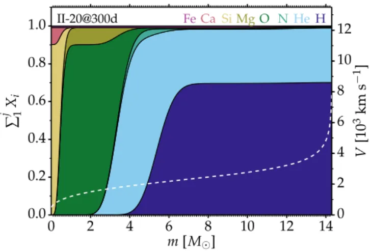
0 2 4 6 8 10 12 14 m [M ] 0.0 0.2 0.4 0.6 0.8 1.0 ∑ j 1X i H He N O Mg Si Ca Fe II-20@300d 0 2 4 6 8 10 12 V [10 3km s − 1]
Fig. 1.Cumulative composition and velocity profiles versus Lagrangian mass in the ejecta of the SN II model based on the 20 M ZAMS star.
The sum for each plotted element i includes the mass fractions for all plotted elements that have a lower atomic mass.
smoothing to broaden the composition profiles to mimic mix-ing. This is a tunable parameter so weak mixing (Gaussian width of 100 km s−1) or strong mixing (Gaussian width of 400 km s−1)
were implemented. For greater freedom, the mixing of56Ni and
other species is chosen to be independent. The adopted initial profile for56Ni is of the form
X(56Ni) ∝ exp(−Y2) with Y = V − VNi
∆VNi ; V ≥ VNi, (4) and connects continuously to a constant 56Ni mass fraction for
V < VNi. The normalization is set by the specified56Ni mass
ini-tially, which is 0.08 M by default. By varying VNi and ∆VNi,
we can enforce various levels of mixing of56Ni and its
daugh-ter elements, and therefore tune the spatial distribution of the absorbed decay power. Figure1illustrates the composition strat-ification for the type II SN ejecta corresponding to the 20 M
ZAMS mass.
2.3. Radiative transfer modeling during the nebular phase with CMFGEN
Using the ejecta configurations described above, we solve the non-local thermodynamic equilibrium (non-LTE) radiative transfer problem with CMFGEN (Hillier & Miller 1998;Dessart & Hillier 2005;Hillier & Dessart 2012). Unlike in recent years, we here assume steady state so that a large number of simulations can be done independently without any knowledge of the pre-vious evolution. We use the fully relativistic transfer equations which are solved in a similar manner to the transfer equations discussed in Hillier & Dessart (2012) and references therein. During the nebular phase, and at the typical velocities encoun-tered in SNe, these give, for all practical purposes, the same results as found using the time-dependent transfer equation.
We treat non-thermal processes as per normal (Dessart et al. 2012; Li et al. 2012). We limit the radioactive decay to the
56Ni chain. For simplicity, we compute the non-local energy
deposition by solving the grey radiative transfer equation with a grey absorption-only opacity to γ-rays set to 0.06 Yecm2g−1,
where Yeis the electron fraction. The model atoms included are:
HI(26,36), HeI(40,51), HeII(13,30), NI(44,104), NII(23,41), OI (19,51), OII (30,111), MgI (39,122), MgII (22,65), SiI
(100,187), SiII(31,59), CaI(76,98), CaII(21,77), FeI(44,136),
FeII(275, 827), FeIII(83, 698), CoII(44,162), CoIII(33,220), NiII (27,177), and NiIII (20,107). The numbers in
parenthe-ses correspond to the number of super levels and full levels employed (for details on the treatment of super levels, seeHillier & Miller 1998).
Obviously, with the limited composition (and associated limited model atom), some lines will not be predicted in our simulations. This includes, for example, NaID so that the fea-ture we predict around 5900 Å is primarily due to HeI5875 Å.
Line blanketing associated with TiIIis also neglected, although
it tends to be much weaker at nebular times. Simulations with a detailed composition and the associated detailed model atom will be used in a forthcoming study.
For the initial conditions needed by CMFGEN, we assume a uniform temperature of 5500 K throughout the ejecta, partial ionization of the gas, and all level populations are at their LTE value. Convergence to the non-LTE solution with a new temper-ature and electron density profile takes about 200 iterations, but only 12h of computing time for a Doppler width of 50 km s−1
(see Sect.3). However, once a given model is converged, vari-ants of that model (for example the same ejecta model but with a different56Ni mass or metallicity, etc.) can be computed quickly
by adopting this converged model as an initial guess for the temperature, level populations, etc.
2.4. Caveats
In our simplified approach, the properties of our adopted ejecta are not accurate nor consistent. We use the pre-SN composi-tion of the main shells (which result from hydrostatic burning) to describe the SN ejecta composition (which results in part from explosive burning), with only one change associated with the presence of a56Ni-rich shell. In practice, this simplification
amounts to introducing a56Ni-rich shell at the base of the ejected
He-core material, leaving the composition of this pre-collapse He core unchanged.
This departs from what may occur in realistic explosions, whereby a large fraction of the Si-rich shell collapses into the compact remnant, while the 56Ni-rich and Si-rich shells are
recreated from explosive burning at the base of the O-rich shell. Strictly speaking, the yields from explosive and hydrostatic burn-ing differ (see, e.g.,Arnett 1996), but these differences are small to moderate. For the current study, the essence is simplification so that we can explore a variety of sensitivities of SN radiation to ejecta properties, focusing on the strength of the strongest lines, the influence of56Ni on Ca ionization and other ejecta properties.
We have already performed simulations with a state-of-the-art ejecta composition (based on the ejecta models ofWoosley & Heger 2007) and these do not yield critical differences that would impact the conclusions drawn in this paper (Dessart & Hillier, in prep.).
Another limitation in our work is that the original shell com-positions are based on MESA simulations that are performed with a small nuclear network of only 21 isotopes. Although incom-plete, it is standard practice in the community for core-collapse SN simulations since it captures the key physics while keeping the computing time small. It is well known that both resolution and network size alter the results of simulations of massive star evolution (Farmer et al. 2016) and explosion (Paxton et al. 2015), but not to an extent that would alter the results of the present study. For example, the s-process can lower the Ca and Fe abun-dance within the O-rich shell. The s-process is ignored by our small network and we find instead that the Ca and Fe mass frac-tions in the O-rich shell are essentially constant in our MESA
simulations. In the SN model s15 ofWoosley & Heger(2007), based on a 15 M star initially, the s-process influences the Ca
and Fe abundances so that they show a depression relative to solar by a factor of 5−10 in the O/C shell, and by a factor of 2−3 in the O/Ne/Mg shell. Ultimately, such features should be prop-erly handled, but we ignore them for the time being. Since the Ca abundance is already 10 000 times lower than the O abundance in the O-rich shell (in the absence of shell merging), a further reduction by a factor of a few does not appear a critical change. When crafting our models, the same assumptions are applied to all ejecta models. Our study focuses on trends, not on accurate quantitative assessments of line fluxes and ejecta yields. Slight offsets in abundances are therefore irrelevant for the conclusions we make.
2.5. Set of simulations
The parameter space that can be explored with our setup is large. One can change parameters in isolation and then try all possible permutations in a systematic way. We choose to be selective and vary parameters that reflect the range of possibilities consistent with our current understanding of stellar evolution and explosion physics. This includes the level of mixing of all species and the separate issue of56Ni mixing, as well as the influence of mass
loss in peeling the star’s envelope, yielding a pre-SN star with various amounts of H-rich material.
In the sections below we present results for simulations in which we varied the adopted Doppler width; the level of mixing either of all species or of56Ni or sometimes both; the mass of
the H-rich envelope in the progenitor; the mass of56Ni; and the
initial star mass. The mass fraction of elements within shells was also varied, in particular to test the influence of the O/Ca mass fraction ratio in the O-rich shell. We varied the metallicity from 0.1 to 2 times solar but found no influence on our results. For all simulations presented here, we set the metallicity to solar. Unless otherwise stated, all simulations adopt a SN age of 300 d.
We do not provide a summary table of all models presented since the models have many properties. Instead, in each section, we emphasize the given parameter that is varied while other parameters are kept identical. Our interest is in the influence of that varying parameter, not the numerous other parameters characterizing each individual model. In each section, the model nomenclature is clear enough to interpret the results and identify each model.
3. Influence of the adopted Doppler width
For nebular phase radiative transfer modeling, most codes use the Sobolev approximation (e.g.,Jerkstrand et al. 2011), which is equivalent to assuming an intrinsic line width of zero. In CMFGEN, this approximation is not used and all lines have a finite width.
Two terms control the intrinsic3broadening of lines. The first
one is associated with the thermal velocity of the corresponding atom or ion, and typically amounts to a few km s−1at the low
temperatures of SN ejecta at nebular times. This velocity width scales with 1/√A, where A is the atomic mass, so the line width of iron group elements is roughly a factor eight narrower than those of hydrogen at the same gas temperature. The other term is associated with turbulence. In our simulations we typically use the same broadening for all lines, and do this by ignoring the 3 Intrinsic in the sense that it applies in the comoving or gas frame, and
is thus present even if the gas is as rest.
thermal contribution and by setting the turbulence to 50 km s−1.
This choice is motivated by speed, and the need to have a “rea-sonable” number of frequency points (still of order 105) to cover
the full spectrum from the far ultraviolet to the far infrared. Tests in this study show that the adopted Doppler width influences the resulting spectra at nebular times The choice of 0 km s−1implied by the Sobolev approximation is the opposite
extreme and is probably not optimal since it prevents any line overlap (and hence interaction) within the Sobolev resonance zone. We adopted a value comparable to that implied by the thermal motions of the gas for IGEs.
In this work, we first converged all models using a fixed Doppler width of 50 km s−1 for all species. This produces a
converged model that is pretty close to the true solution (the essential part of the solution being the converged temperature, ionization, and level populations). This converged model is then used as initial conditions for a new CMFGEN model in which a fixed Doppler width of 2 km s−1is used for all species (in cases
where the impact on the gas properties was large, this reduction was done in a few steps)4. The frequency grid is set so that all
lines are resolved, irrespective of their widths. So, reducing the Doppler width of lines from 50 to 2 km s−1leads to an increase
in the number of frequency points from 49 352 to 841 208 in the present simulations. This model takes much longer per iteration but it requires fewer iterations to converge since it starts with a better guess. With the lower Doppler width, the temperature and ionization are slightly modified and cause a sizable change in the strength of the strongest lines and the FeIIemission for-est around 5000 Å. The evolution can be nonlinear, in the sense that reducing the line Doppler width can yield a non-monotonic increase or decrease in the flux of [OI] λλ 6300, 6364, Hα, or
[CaII] λλ 7291, 7323.
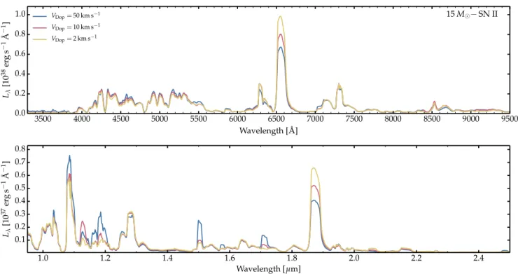
Figure2shows the influence on the optical and near-infrared spectrum of changing the Doppler width from 50 to 10 and 2 km s−1 in a strongly mixed ejecta model corresponding to
a 15 M progenitor. Reducing the Doppler width leads to a
strengthening of Hα and Pa α (and a weakening of the near-infrared MgIlines) which may have resulted from the increase
of the electron density and the H ionization in the recombined H-rich layers of the ejecta. The same test in a model with weaker mixing would yield a different impact because the modified mix-ing has a strong influence on the emergent spectrum. So, for example, in a weakly mixed model, the reduction of the Doppler width leads to a reduction of HeI7068 Å and MgIlines in the
near infrared, a strengthening of the CaIIlines in the optical, but has little impact on the HIlines. It is thus important to realize
that the adopted Doppler width can influence nebular line ratios. The influence of line overlap on non-LTE processes is well documented. For example, overlap of an OIII line with HeII
Ly α in planetary nebula leads to anomalous line strengths for several optical OIIIlines (e.g.,Bowen 1934;Osterbrock 1989).
In some O stars the chance overlap of FeIV lines with the HeI
resonance transition at 584 Å influences the strength of HeI
sin-glet transitions in the optical (particularly those involving the 1s 2p1Po level; Najarro et al. 2006). Another example, is the
overlap of an OIline with Ly β which can, for example, influence
the strength of OIλ8446 (e.g.,Osterbrock 1989). As discussed byJerkstrand et al.(2012), a significant concern for modeling the nebular phase of Type IIP SNe is the overlap of some FeIIand 4 We also run tests in which the Doppler width was determined based
on the species atomic mass and a microturbulent velocity of 2 km s−1.
This is similar to using a Doppler width of ∼10 km s−1for H, 5 km s−1
3500 4000 4500 5000 5500 6000 6500 7000 7500 8000 8500 9000 9500 Wavelength [ ˚A] 0.0 0.2 0.4 0.6 0.8 1.0 Lλ [10 38er g s − 1˚ A − 1] 15 M − SN II VDop=50 km s−1 VDop=10 km s−1 VDop=2 km s−1 1.0 1.2 1.4 1.6 1.8 2.0 2.2 2.4 Wavelength [µm] 0.1 0.2 0.3 0.4 0.5 0.6 0.7 0.8 Lλ [10 37er g s − 1˚ A − 1]
Fig. 2.Influence of the adopted Doppler width on the resulting optical and near-infrared spectra for a SN II model arising from a 15 M progenitor.
A weak mixing of all species is used except for56Ni for which we adopt a strong mixing. The increase in Hα line flux with decreasing V Dopis at
the expense of a decrease in flux from a forest of FeIIlines in the 4000−6000 Å region. Other lines affected are HeI1.083 µm, OI1.129 µm, FeI lines around 1.165 µm, MgIlines at 1.183, 1.502, 1.577, 1.711, HI1.875 µm. Note that about 70% of the total flux falls in the optical range.
OIlines with Ly α and Ly β. We verified the cause of the spectral changes by running test calculations which used a Doppler width of 50 km s−1and modified model atoms for which we artificially
reduced the oscillator strengths (effectively setting them to zero) of FeIIand OIlines overlapping with Ly α and Ly β.
4. Discussion of model results from a 20 M type II
SN model
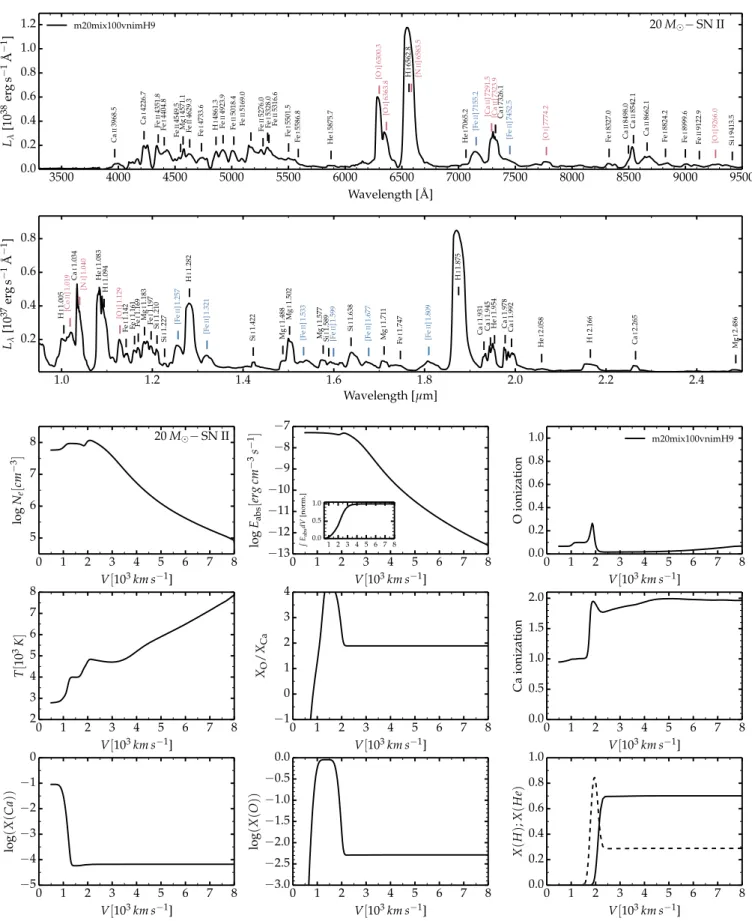
We first describe the case of a type II SN ejecta from a 20 M
ZAMS star. The model is named m20mix100vnimH9, where “mix100” means that the Gaussian smoothing uses a character-istic width of 100 km s−1(this mixing is applied to all species),
“vni” means that the additional mixing applied to 56Ni was
strong (VNi=2500 km s−1and ∆VNi=1000 km s−1; see Eq. (4)),
and “mH9” means that the pre-SN progenitor had a 9 M
H-rich outer shell. The ejecta has a kinetic energy of 1051erg and
contains 0.08 M of56Ni initially.
A summary of results for this reference model is shown in Fig. 3. The top two panels show the optical and near-infrared spectral properties. Throughout the paper, we show luminosi-ties Lλ(in erg s−1Å−1) rather than scaled or normalized fluxes
because its integral over wavelength yields the bolometric lumi-nosity and thus the decay power absorbed by the ejecta. Varia-tions in56Ni mass or γ-ray trapping efficiency will yield different
brightnesses, which can be assessed from Lλ. The bottom panels
show various properties of the ejecta, including the ionization level (electron density, O and Ca ionization), the temperature, the composition (for H, He, O, or Ca, and for the ratio of O/Ca, which is relevant for the [OI] λλ 6300, 6364 doublet strength in core-collapse SNe; see next section), and the profile of the decay power absorbed.
The total radial electron scattering optical depth for this 300 d-old ejecta is 0.4. Under such conditions, the ejecta no
longer traps radiation so the energy balance is set by the distri-bution of decay power absorbed at that time in the ejecta and the reprocessing of this power by the gas in the form of low-energy, mostly optical, photons – whatever is absorbed is instantaneously radiated and the balance is zero. Because of the strong56Ni
mix-ing and some non-local energy distribution, the decay power is absorbed throughout the ejecta. Relative to the total energy absorbed, the Si-rich layers below 1000 km s−1 get ∼20%, the
O-rich layers between 1000 and 1800 km s−1get ∼40%, the
He-rich layers between 1800 and 2100 km s−1 get ∼10%, and the
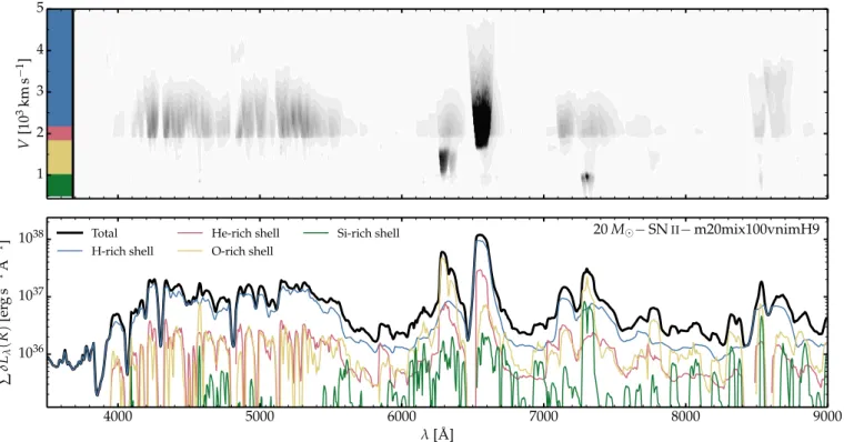
outer H-rich layers receive the remaining ∼30%. Interestingly, the amount of radiation escaping to infinity and arising from these shells is very different, as shown in Fig.4. In other words, there is a significant reprocessing of these low-energy photons by the ejecta.
Figure 4 illustrates the spatial origin of the emerging flux and more specifically the quantity δLλ(R) – it illustrates the
loca-tion of the last interacloca-tion (not necessarily the localoca-tion where the photon was originally emitted). The fractional contribution to the total flux at wavelength λ from a narrow ejecta shell at radius R is:
δLλ(R) = 8π2
Z
∆z η(p, z, λ) e−τ(p,z,λ) p dp , (5)
where ∆z is the projected shell thickness for a ray with impact parameter p, η is the emissivity along the ray at p and z, and τ is the total ray optical depth at λ (i.e., the integral is performed in the observer’s frame) at the ejecta location (p, z). Figure 4
shows that the bulk of the flux emerges from the H-rich ejecta layers, which is 61% of the total and thus about twice as much as deposited by γ-rays and positrons. The He-rich layers radi-ate 15% of the total, compared to the 10% of the decay power that they absorb. The O-rich (Si-rich) layers radiate 20% (4%) of the total, compared to the 40% (20%) of the decay power that
3500 4000 4500 5000 5500 6000 6500 7000 7500 8000 8500 9000 9500 Wavelength [ ˚A] 0.0 0.2 0.4 0.6 0.8 1.0 1.2 Lλ [10 38 er g s − 1˚ A − 1] 20 M − SN II Ca II 3968.5 Ca I 4226.7 Fe II 4351.8 Fe I 4404.8 Fe II 4549.5 Mg I 4571.1 Fe II 4629.3 Fe I 4733.6 H I 4861.3 Fe II 4923.9 Fe II 5018.4 Fe II 5169.0 Fe II 5276.0 Fe I 5328.0 Fe II 5316.6 Fe I 5501.5 Fe I 5586.8 He I 5875.7 [O I ]6300.3 [O I ]6363.8 H I 6562.8 [N II ]6583.5 He I 7065.2 [Fe II ]7155.2 [Ca II ]7291.5 [Ca II ]7323.9 Ca I 7326.1 [Fe II ]7452.5 [O I ]7774.2 Fe I 8327.0 Ca II 8498.0 Ca II 8542.1 Ca II 8662.1 Fe I 8824.2 Fe I 8999.6 Fe II 9122.9 [O I ]9266.0 Si I 9413.5 m20mix100vnimH9 1.0 1.2 1.4 1.6 1.8 2.0 2.2 2.4 Wavelength [µm] 0.2 0.4 0.6 0.8 Lλ [10 37er g s − 1˚ A − 1] H I 1.005 [CoII ]1.019 Ca I 1.034 [N I ]1.040 He I 1.083 H I 1.094 [O I ]1.129 Fe I 1.142 Fe I 1.161 Fe I 1.169 Mg I 1.183 Fe I 1.197 Si I 1.210 Si I 1.227 [Fe II ]1.257 H I 1.282 [Fe II ]1.321 Si I 1.422 Mg I 1.488 Mg I 1.502 [Fe II ]1.533 Mg I 1.577 Si I 1.589 [Fe II ]1.599 Si I 1.638 [Fe II ]1.677 Mg I 1.711 Fe I 1.747 [Fe II ]1.809 H I 1.875 Ca I 1.931 Ca I 1.945 He I 1.954 Ca I 1.978 Ca I 1.992 He I 2.058 H I 2.166 Ca I 2.265 Mg I 2.486 0 1 2 3 4 5 6 7 8 V[103km s−1] 5 6 7 8 log Ne [c m − 3] 20 M − SN II 0 1 2 3 4 5 6 7 8 V[103km s−1] 2 3 4 5 6 7 8 T [10 3K ] 0 1 2 3 4 5 6 7 8 V[103km s−1] −13 −12 −11 −10 −9 −8 −7 log Eabs [e rg cm − 3s − 1] 1 2 3 4 5 6 7 8 0.0 0.5 1.0 R E abs dV [norm.] 0 1 2 3 4 5 6 7 8 V[103km s−1] −1 0 1 2 3 4 XO / XCa 0 1 2 3 4 5 6 7 8 V[103km s−1] 0.0 0.2 0.4 0.6 0.8 1.0 O ionization m20mix100vnimH9 0 1 2 3 4 5 6 7 8 V[103km s−1] 0.0 0.5 1.0 1.5 2.0 Ca ionization 0 1 2 3 4 5 6 7 8 V[103km s−1] −5 −4 −3 −2 −1 0 log (X (C a) ) 0 1 2 3 4 5 6 7 8 V[103km s−1] −3.0 −2.5 −2.0 −1.5 −1.0 −0.5 0.0 log (X (O )) 0 1 2 3 4 5 6 7 8 V[103km s−1] 0.0 0.2 0.4 0.6 0.8 1.0 X (H ); X (H e)
Fig. 3.Illustration of properties for the reference model m20mix100vnimH9 discussed in Sect.4. In this and similar figures, the top panels show the luminosity Lλ(integrating over wavelength yields the bolometric luminosity) in the optical (upper) and the near infrared (lower). The line
identifications are indicative only since in numerous cases multiple lines contribute (we give the primary component to most features). Forbidden lines are shown in red for all ions and atoms apart from Fe (shown in blue). Bottom panels: some ejecta properties computed with CMFGEN.
4000 5000 6000 7000 8000 9000 λ[ ˚A] 1036 1037 1038 ∑ δL λ ( R ) [er g s − 1˚ A − 1] 20 M −SNII−m20mix100vnimH9 Total H-rich shell He-rich shell O-rich shell Si-rich shell 1 2 3 4 5 V [10 3km s − 1]
Fig. 4.Illustration of the spatial regions (here shown in velocity space) contributing to the emergent flux in a 20 M type II SN model characterized
by weak mixing for all non-IGE species, strong mixing for IGE species, and with a 9 M H-rich envelope mass (model m20mix100vnimH9). Top
panel: observer’s frame luminosity contribution δLλ,R (Eq. (5); the map maximum is saturated at 20% of the true maximum to bias against the
strong Hα line and better reveal the origin of the weaker emission) versus wavelength and ejecta velocity. The four contributing shells in this type II SN model are clearly seen (see vertical colored stripe at left), although the H-rich layers contribute most of the emergent flux. Bottom panel: emergent luminosity integrated over each shell, together with the total luminosity. In this model, the fraction of the total power emerging from the Si-rich, O-rich, He-rich and H-rich shells is 4, 20, 15, and 61%, respectively. This illustrates the contribution to the emergent total flux from the main ejecta shells (this may also be inferred from the width of lines but complicated when multiple regions contribute or when there is line overlap). Note that with our approach, IGEs are present in all shells and thus FeIand FeIIflux contribution is present throughout the ejecta. One can also see that the flux from the Si-rich shell is mostly radiated by CaIand CaII(together with FeIand FeII, rather than by the dominant species Si).
they absorb. In the absence of optical depth effects, the power from each shell would be equal to the decay power absorbed in each corresponding shell. With a total electron-scattering opti-cal depth of 0.4 at the SN age of 300 d, the ejecta is not thin. It is not optically thick enough to cause radiation storage and diffusion with a sizable delay, but it is optically thick enough to cause strong reprocessing of UV and blue optical photons, which benefits the emission from the outer layers in this model. Such optical depth effects and their wavelength-dependent impact are illustrated in Fig.5.
Figure4also illustrates the complicated line formation pro-cess at nebular times. It helps in solving the problem of line overlap since a feature may appear broad with a narrow peak because it forms throughout the ejecta (from small to large velocities) or because it forms in a single narrow shell but overlaps with adjacent lines. Let us consider the formation of the strongest optical lines, which are mostly forbidden. The [OI] λλ 6300, 6364 doublet forms primarily in the O-rich shell
(yellow line in Fig.4), with a small contribution at large velocity from the H-rich shell (blue line) and a small contribution at low velocity from the He-rich shell (red line). This contribution from the He shell arises from our imposed mixing and is confined to the region at the interface between the two shells (Fig.1).
The [CaII] λλ 7291, 7323 doublet forms throughout the
ejecta – from the outer part of the Si-rich shell and the inner part of the O-rich shell, and from the H-rich shell (very broad component). The [CaII] λλ 7291, 7323 doublet emission extends
4000 5000 6000 7000 8000 9000 Wavelength [ ˚A] −1 0 1 2 3 4 5 6 7 log τ (V > Vmin ) Vmin=0 km s−1 Vmin=1780 km s−1 Vmin=2150 km s−1
Fig. 5.Illustration of the total (i.e., accounting for all opacity sources) radial optical depth integrated from the outer ejecta boundary to the innermost boundary (i.e., the base of the ejecta; blue), to the He/O shell interface at 1780 km s−1(red), and to the He/H shell interface at
2150 km s−1(yellow) for the reference model m20mix100vnimH9. up to 7400 Å because of the contribution from the H-rich shell but also because of the influence of electron scattering in the fast moving H-rich layers. The emission further to the red is due to FeII(strongest component at 7452 Å). The He-rich shell,
which is nearly exclusively He with a small amount of N, con-tributes mostly through the emission of NII6548 Å, but this
emission overlaps with the strong and broader Hα line seen at all times in SNe II. The NII identification is thus nontrivial in SNe II, but it is observed and explained in some SNe IIb (Jerkstrand et al. 2015b). Below 6000 Å, most of the flux emerges from the H-rich layers and stems mostly from FeIand FeIIline emission (with a mix of permitted and forbidden transitions). The strongest FeIIline is an isolated forbidden line at 7155.2 Å.
There is a weak MgI4571 Å line from the O-rich shell (as well as the OI 7774 Å further to the red). The nucleosynthetic signa-tures of the explosion and the pre-SN evolution are thus quite limited, with the main features being [OI] λλ 6300, 6364 and [CaII] λλ 7291, 7323. A more extensive list of line identifications
is provided in the upper panels of Fig.3.
In the near infrared, the synthetic spectrum shows lines from the Paschen series of HI, HeI1.083 µm, OI1.129 µm,
MgI1.488, 1.502 and 1.711 µm, SiI at 1.227 and 1.422 µm,
numerous CaI lines just short of 2 µm, as well as numerous
FeIand FeII lines spread throughout the near infrared. These identifications are often ambiguous since most features are a composite of different lines.
One aspect that controls the radiative properties of the nebular phase spectrum is the ionization (shown for O and Ca in the bottom panels of Fig.3). Here, the mass density is con-stant below about 2000 km s−1so the variations of the electron
density below 2000 km s−1 reflect the change in ionization and
mean atomic weight as we proceed through the He-rich shell, the O-rich shell, and the Si-rich shell. Oxygen is primarily neutral in the O-rich shell but Ca is once ionized in the Si-rich shell. The jump in ionization and temperature in the He-rich shell arises because the dominant species in that shell (i.e., He) is a poor coolant.
At all depths in the ejecta, the heating source is radioactive decay. However, because of the stratification in composition and the range of densities between inner and outer ejecta, the sources of cooling vary drastically with depth. In the H-rich layers, we find that the cooling is done through non-thermal excitation and ionization (primarily in association with HI, and by a factor of
ten weaker with HeI), and collisional excitation of FeII(and to
a lesser extent MgIIand OI). In the He-rich shell, the cooling
is done through collisional excitation of FeIIand non-thermal
processes tied to HeI. In the O-rich shell, cooling arises primar-ily from collisional excitation of OIand non-thermal processes
tied to OI, and then from collisional excitation of MgI and FeII. In the Si-rich shell, the cooling is done primarily through
collisional excitation of CaII as well as CaI, plus non-thermal
processes tied to SiI. Figure6 illustrates these various cooling
components at different ejecta depths in this reference model m20mix100vnimH9.
The above results need to be considered in view of our assumptions. First, the ejecta composition is limited to H, He, N, O, Mg, Si, Ca, and the56Ni decay chain elements so the lines
present in the models are by design limited to these elements (in their neutral or once ionized state). The second aspect is that we adopt a strong mixing of56Ni with a weak mixing of the other
(lighter) elements. This gives some preference to the intermedi-ate and high velocity layers of the ejecta (although we have seen that the outer layers do a lot of reprocessing of the radiation emit-ted from the inner layers). Finally, because of the weak mixing of species other than56Ni, the metal-rich layers retain an onion-like
shell structure. With macroscopic mixing only, material from all shells in the pre-SN star would coexist at a given velocity. The
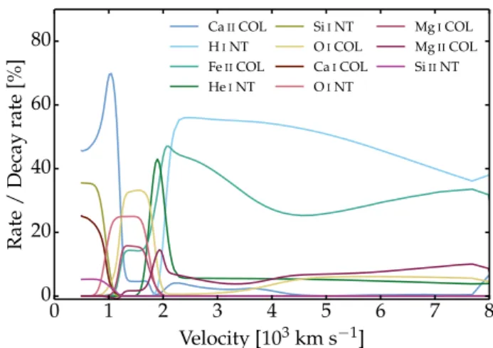
0 1 2 3 4 5 6 7 8 Velocity [103km s−1] 0 20 40 60 80 Rate / Decay rate [%] CaIICOL HINT FeIICOL HeINT SiINT OICOL CaICOL OINT MgICOL MgIICOL SiIINT
Fig. 6. Illustration of the main cooling processes balancing the radioactive decay heating at all ejecta depths in the reference model m20mix100vnimH9. We show each dominant cooling rate (stepping down from the rate having the largest peak value at any depth) nor-malized to the local heating rate. The term “NT” stands for non-thermal processes (in this context non-thermal excitation and ionization) and “COL” stands for collisional processes (i.e., collisional excitation).
reprocessing of radiation from the inner ejecta by the various lumps of material would be much more complex than in the present configuration of shells of distinct composition stacked on top of each other.
5. Importance of the Ca mass fraction in the O-rich shell
Converting line strengths into abundances of the associated ion and species is one of the principal goals of nebular phase spec-troscopy for any type of SN. There are however many caveats associated with this task. First, the radiation emitted by any ion is very dependent on the atomic physics of that ion. Second, it depends on the efficiency of other species that are radiating from the same region. Third, it depends on where the radioactive decay power emitted is absorbed by the ejecta. Hence, a funda-mental aspect of nebular line emission is how the56Ni is mixed
through the ejecta and how far the emitted γ-rays can travel in the ejecta.
Having determined the non-local distribution of this decay power and which fraction of the total is shared between each dominant ejecta shell (H-rich shell, He-rich shell, O-rich shell, and the Si-rich shell), the radiation emitted in each shell will occur through the lines that have the strongest cooling power. The cooling efficiency of a given forbidden line depends of course on the abundance of the corresponding ion (hence a func-tion of mass fracfunc-tion and ionizafunc-tion level), but also on atomic properties of the ion levels (oscillator strength, critical density, etc.). In practice, type II SN ejecta exhibit a wide disparity in ion-ization, composition, and density, and the various constituents have widely different atomic properties so that even trace ele-ments can dominate the cooling of the gas (the same holds in HII
regions, whose cooling is controlled to a large extent by emis-sion in lines of NII, OIIand OIII while the dominant species
are instead H and He;Osterbrock 1989).
Below, we discuss the case of the doublet forbidden transi-tions [OI] λλ 6300, 6364 and [CaII] λλ 7291, 7323 because they
are the strongest optical lines in type II SN spectra at nebular times (if we exclude Hα) and also because they are routinely
Table 3. Atomic properties associated with the [OI] λλ 6300, 6364 and [CaII] λλ 7291, 7323 doublet transitions.
Species Transition Levels λ Aul Υ(T4= 0.5) Ne(crit)(T4= 0.5)
[Å] [s−1] [s−1] [cm−3] OI 3P2–1D2 1−4 6300.3 5.096 × 10⁻³ OI 3P1–1D2 2−4 6363.8 1.639 × 10⁻³ 0.124(T4/0.5)(a) 2.2 × 10⁶ OI 3P0–1D2 2−4 6391.7 7.230 × 10⁻⁷ CaII 2S1/2–2D3/2 1−2 7323.9 0.795 4.58 5.8 × 10⁶ CaII 2S1/2–2D5/2 1−3 7291.5 0.802 6.79 5.8 × 10⁶ Notes. (a)The value listed is the total collision strength for the3P to1D transition.
used to set constraints on nucleosynthesis and progenitor proper-ties. We then present simulations in which various amounts of Ca are introduced into the O-rich shell. These simulations show the strong impact Ca can have on OIline emission. We then discuss
the implications and comment on previous work. 5.1. The cooling power of [OI]λλ 6300, 6364 and
[CaII]λλ 7291, 7323
Let us consider a small gas volume of uniform composition with a gas temperature T (or T4 when expressed in units of 104K)
and electron density Ne. Below, we study how the emissivity of
(or the cooling rate associated with) the [OI] λλ 6300, 6364
dou-blet compares with that of the [CaII] λλ 7291, 7323 doublet. We
assume optically-thin emission in this simplified analysis. This approximation may not hold strictly, in particular for large Ca densities.
The collisional de-excitation rate per unit volume per unit time from the upper level “u” to the lower level “l” is given by NuCul= 8.67 × 10 −8 √T 4 Υlu gu NeNu, (6)
where Nu is the upper level population and Υlu is the effective
collision strength for the transition (data for collision strengths are taken fromMendoza 1983for O Iand fromMeléndez et al. 2007for Ca II; energy levels are from NIST, while Aulvalues for
OIare fromOsterbrock 1989and those for CaIIare similar to those inLambert & Mallia 1969)5.
At the critical density, this rate is equal to NuAul. Thus
Ne(crit) = 1.16 × 10⁷guAul
√T
4
Υlu cm
−3. (7)
For OIwe sum the Aul values for the two transitions, to get a
critical density. For Ca II, we treat the upper level as a single level (A = P guAul/Pgu, and Υ = P Υlu). In the following, we
assume OI and Ca IIare the dominant ionization stages, and
5 The values listed in the table are those used in the present
calcu-lations. Experimental lifetime measurements, and theoretical calcula-tions, suggest that a better estimate for A for the CaIItransitions is 1.1 (see Meléndez et al. 2007). The value listed in the NIST database is 1.3 (Kramida & NIST ASD Team 2019). It comes from a calculation by
Osterbrock(1951) and has an indicated error of greater than 50%. The OIvalues are slightly lower than those in the NIST databaseKramida
& NIST ASD Team(2019) (5.6 × 10⁻³and 1.8 × 10⁻³; E < 7%)
how-ever Baluja et al. (1988) suggest even higher values (6.7 × 10⁻³ and
2.3 × 10⁻³). While the adoption of different cross-sections will (slightly)
alter line strengths, they will not affect any of the conclusions made in this paper.
that levels other than those listed above can be neglected. We use the atomic properties listed in Table3.
We may consider two limiting cases for the strength of these forbidden lines, corresponding to electron densities much higher or much lower than the critical density of the transition.
Case 1: Ne Ne(crit).In this case we can assume the upper
level is in LTE relative to the ground state. Thus, the OI line
emissivity is given by η(OI) = hνulNuAul= gu gl hνulAulNO exp − hνul kT ! , (8) or η(OI) = 5 9hνulAulNOexp λ(µm)T−1.43884 ! . (9)
Similarly, for the CaIIline (gu/gl=10/2), we have
η(CaII) = 5 hνulAulNCaexp −1.4388
λ(µm)T4
!
. (10)
Integrating these line emissivities over the O-rich shell volume yields the line luminosities L. Taking the ratio we obtain,
L(OI) L(CaII) =1.08 × 10 −3NO NCaexp −0.309 T4 ! . (11)
Case 2: Ne Ne(crit).In this case, the line emissivity is
η = 8.67 × 10√ −8 T4 Υlu gl NeNlhνulexp −1.4388 λ(µm)T4 ! , (12)
since every excitation gives a line photon. Thus, the ratio of line luminosities is now L(OI) L(CaII) =2.81 × 10 −3NO NCaexp −0.309 T4 ! . (13)
In this case we could add a factor like (T4/0.5)0.5 since the OI
collision strength grows faster than that of CaII. A factor of 2.5
(i.e., 40/16) is introduced if we express Eqs. (11) and (13) with mass fractions.
In the optically-thin limit, the luminosity contrast between these two lines would be huge if Ca was as abundant as O in the O-rich shell (in practice, line optical depth effects would reduce this CaIIemission). Equations (11) and (13) show that the CaII
line would dominate over the OIline if the Ca abundance is at least ∼1% of the O abundance in the O-rich shell. This situation does not occur if Ca has the solar abundance in the O-rich shell,
but the merging of the Si-rich and O-rich shells may change this. The impact would depend on the mass of the Si-rich and O-rich shells in the pre-SN star (and prior to merging). These shells masses grow with the progenitor mass, with a 2−3 times faster increase for the O-rich shell mass.
5.2. The influence of O/Ca in the O-rich shell: numerical simulations with CMFGEN
Using as a reference the model m20mix100mH9 produced with the prescriptions stipulated in Sect.2.2, we produce three other models in which the Ca mass fraction in the O-rich shell is raised from its solar value of 6.4 × 10⁻⁵ to 0.0007 (model suffix Cal),
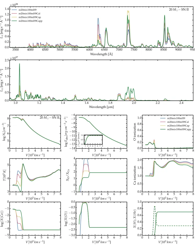
0.007 (suffix Cap), and finally 0.07 (suffix Capp). The CMFGEN results for both the optical and near-infrared radiation and the gas properties are shown in Fig.7.
As expected, raising the Ca mass fraction in the O-rich shell has a dramatic effect on the [OI] λλ 6300, 6364 doublet strength
(note that the distribution of the decay power absorbed is the same in all four models since we switch O for Ca but at constant density and mass; see middle panel). The effect is present even for an O/Ca mass fraction ratio in the O-rich shell of 1000. The influence on Hα is negligible, which is expected since the H-rich layers were not modified. The CaIIlines are strengthened, but
for the higher Ca enhancement, their strength decreases to the benefit of CaIlines (mostly present in the near infrared; bottom spectral panel of Fig.7). The ionization is still primarily Ca+, but
there is a small inflection in the ionization, the electron density, and in the temperature in the O-rich shell. The most likely reason for this saturation and even reduction of the CaIIflux is that both
doublet components are optically thick (Fig.8). 5.3. Implications and comparison to previous work
A number of points need to be made at this stage. Rather than being secondary and irrelevant, the Ca mass fraction in the O-rich shell is a critical matter because it affects the OIdoublet, which is used for constraining the progenitor mass. In the above experiment, the mass of the O-rich shell is the same in all four ejecta models and yet the OI doublet flux varies by a factor of
about five just by tuning the Ca/O ratio in the O-rich shell. Some of the adopted Ca mass fractions in this experiment are probably too large. However, stellar evolution simulations frequently produce a large Ca mass fraction in the O-rich shell. This occurred in half the MESA simulations we ran for this study. The cause is the merging of the Si-rich shell and the O-rich shell during Si burning, producing a Ca mass fraction of a few 0.001 in the O-rich shell, so that the O/Ca mass fraction ratio drops by a factor of 100 compared to the case of no shell merging (the total Ca mass is however unchanged by this merging). A similar feature was observed byFransson & Chevalier(1989) in some of their models (computed with KEPLER and presented inEnsman & Woosley 1988).Collins et al. (2018) report a higher occur-rence of merging for the O, Ne, and C burning shells in higher mass progenitors between 16 and 26 M , yielding a large Si mass
fraction in a large part of the O-rich shell – this is the same as what we observe in our MESA simulations. Similarly, Yoshida et al.(2019) obtain distinct composition profiles within the Si-and O-rich shells depending on the adopted convective overshoot strength and progenitor mass.
In the absence of such a merging, the Ca mass fraction in the O-rich shell is typically at the original value on the ZAMS (i.e., at the solar metallicity in our models; see Sect. 2.4 for departures from a solar value), but one can wonder whether this
feature would persist in 3D hydrodynamical simulations treating physically the processes of convection and overshoot. Even with strong overshoot from the Si-rich shell, it is not clear that mixing could take place down to the microscopic level given the short time until collapse and explosion (typically a day from the onset of Si burning; see, e.g.,Arnett 1996orCollins et al. 2018) – the mixing might instead be partial and truncated at some spatial scale.
The origin of CaIIemission is a related issue. In the
exper-iment above, if the Ca mass fraction is large in the O-rich shell (say with a ∼ 0.01 mass fraction), most of the power absorbed by the O-rich shell is radiated through CaIIlines (this process can
be mitigated by line optical depth effects). Otherwise, we obtain CaIIemission from the Si-rich shell, the interface between the
Si-rich shell and the O-rich shell (where the Ca mass frac-tion is around or above 0.01), and from the He-rich and H-rich shells.
Li & McCray(1993) and others argue that the CaIIemission
arises primarily from the Ca in the H-rich envelope. The main limitation for Ca emission from the rich shell is that the Si-rich shell is of low mass, and hence it absorbs a small fraction of the total decay power. Even if Ca were the sole coolant in that Si-rich shell, the total power that it would radiate would be a small fraction of the total, typically smaller than the power absorbed in the H-rich layers (though this can depend on the mass of the CO core and the level of mixing). More importantly, the main competitor is the CO core mass, which in massive progenitors may absorb most of the decay power (again a function of mix-ing, etc.). Whether Ca emission comes from the H-rich envelope is not just a matter of Ca being a strong coolant. It depends pri-marily on where the decay power is absorbed. For a larger He core mass (a higher mass progenitor), for a larger ejecta mass, or for a weaker level of56Ni mixing, a larger fraction of the decay
power may be absorbed in the core rather than the H-rich layers. In this situation, the H-rich ejecta layers would only reprocess the radiation impinging from below.
The origin of the CaII emission would be altered in the
case of Ca pollution into the O-rich shell prior to core collapse. This would enhance the [CaII] λλ 7291, 7323 doublet flux at the
expense of the [OI] λλ 6300, 6364 doublet flux. If the process of shell merging had a higher occurrence rate in higher mass progenitors (Collins et al. 2018), it would provide a natural expla-nation for the lack of SNe II with strong [OI] λλ 6300, 6364 at
nebular times, and inferred progenitor masses below 17 M . 6. Influence of the H-rich envelope mass
In our toy setup, we either force the ejecta mass to be 10 M
(and we adjust the H-rich envelope mass) or we force the H-rich envelope mass to be 9 M (and we adjust the ejecta mass to be
the sum of the H-rich envelope mass plus the He-core mass). The latter might be a good description of single stars initially in the mass range between 12 and about 20 M and the latter more
suit-able to higher mass stars but still dying as RSGs (Woosley et al. 2002;Dessart & Hillier 2019b). Since we assume the same ejecta kinetic energy, variations in total mass or envelope structure will impact the distribution of elements in velocity space.
Figure 9 illustrates the impact of the H-rich envelope mass of the progenitor (or the total mass of the ejecta) for a 25 M progenitor model (this defines the core properties).
The low-envelope mass model is m25mix100vni (total ejecta mass is 9.9 M ) and the high-envelope mass model is
m25mix100vnimH9 (total ejecta mass is 16.7 M ) in our
3500 4000 4500 5000 5500 6000 6500 7000 7500 8000 8500 9000 9500 Wavelength [ ˚A] 0.0 0.2 0.4 0.6 0.8 1.0 1.2 1.4 Lλ [er g s − 1˚ A − 1] ×1038 20 M − SN II m20mix100mH9 m20mix100mH9Cal m20mix100mH9Cap m20mix100mH9Capp 1.0 1.2 1.4 1.6 1.8 2.0 2.2 2.4 Wavelength [µm] 0.0 0.5 1.0 1.5 2.0 2.5 Lλ [er g s − 1˚ A − 1] ×1037 0 1 2 3 4 5 6 7 8 V[103km s−1] 4 5 6 7 8 log Ne [c m − 3] 20 M − SN II 0 1 2 3 4 5 6 7 8 V[103km s−1] 3 4 5 T [10 3K ] 0 1 2 3 4 5 6 7 8 V[103km s−1] −14 −13 −12 −11 −10 −9 −8 −7 −6 log Eabs [e rg cm − 3s − 1] 1 2 3 4 5 6 7 8 0.0 0.5 1.0 R E abs dV [norm.] 0 1 2 3 4 5 6 7 8 V[103km s−1] −1 0 1 2 3 4 XO / XCa 0 1 2 3 4 5 6 7 8 V[103km s−1] 0.0 0.2 0.4 0.6 0.8 1.0 O ionization m20mix100mH9 m20mix100mH9Cal m20mix100mH9Cap m20mix100mH9Capp 0 1 2 3 4 5 6 7 8 V[103km s−1] 0.0 0.5 1.0 1.5 2.0 Ca ionization 0 1 2 3 4 5 6 7 8 V[103km s−1] −5 −4 −3 −2 −1 0 log (X (C a) ) 0 1 2 3 4 5 6 7 8 V[103km s−1] −3.0 −2.5 −2.0 −1.5 −1.0 −0.5 0.0 log (X (O )) 0 1 2 3 4 5 6 7 8 V[103km s−1] 0.0 0.2 0.4 0.6 0.8 1.0 X (H ); X (H e)
Fig. 7.Similar to Fig.3, but now showing variants of model m20mix100mH9 in which the Ca mass fraction is progressively increased in the O-rich shell by powers of ten and starting from about 7 × 10⁻⁵, the solar metallicity value (the Ca mass fraction profile is shown in the bottom left panel).
Notice the dramatic reduction on the [OI]/[CaII] line ratio as the Ca abundance is increased. Even in the richest Ca model, the Ca mass is still less than 10% of the O mass.
![Table 3. Atomic properties associated with the [O I ] λλ 6300, 6364 and [Ca II ] λλ 7291, 7323 doublet transitions.](https://thumb-eu.123doks.com/thumbv2/123doknet/14792568.602054/12.892.154.736.153.296/table-atomic-properties-associated-λλ-λλ-doublet-transitions.webp)