Simple Method for the Solution of Loaded Plate Problems

Publisher’s version / Version de l'éditeur:

Technical Translation (National Research Council of Canada), 1965

READ THESE TERMS AND CONDITIONS CAREFULLY BEFORE USING THIS WEBSITE.

https://nrc-publications.canada.ca/eng/copyright

Vous avez des questions? Nous pouvons vous aider. Pour communiquer directement avec un auteur, consultez la

première page de la revue dans laquelle son article a été publié afin de trouver ses coordonnées. Si vous n’arrivez pas à les repérer, communiquez avec nous à PublicationsArchive-ArchivesPublications@nrc-cnrc.gc.ca.

Questions? Contact the NRC Publications Archive team at

PublicationsArchive-ArchivesPublications@nrc-cnrc.gc.ca. If you wish to email the authors directly, please see the first page of the publication for their contact information.

NRC Publications Archive

Archives des publications du CNRC

For the publisher’s version, please access the DOI link below./ Pour consulter la version de l’éditeur, utilisez le lien DOI ci-dessous.

https://doi.org/10.4224/20386679

Access and use of this website and the material on it are subject to the Terms and Conditions set forth at

Simple Method for the Solution of Loaded Plate Problems

Schleeh, W.

https://publications-cnrc.canada.ca/fra/droits

L’accès à ce site Web et l’utilisation de son contenu sont assujettis aux conditions présentées dans le site LISEZ CES CONDITIONS ATTENTIVEMENT AVANT D’UTILISER CE SITE WEB.

NRC Publications Record / Notice d'Archives des publications de CNRC:

https://nrc-publications.canada.ca/eng/view/object/?id=df9cb8ef-7ef7-4e26-b6c8-8e47a610b0cc https://publications-cnrc.canada.ca/fra/voir/objet/?id=df9cb8ef-7ef7-4e26-b6c8-8e47a610b0cc

The Division of Building Researoh has been interested in

precast concrete construct1on for a number of years. In

con-crete design, both normally re1nforced and pre-stressed, the stress d1stribution in deep beams and locally in the areas near concentrated loads is of great 1mportance 1n determining the amount and distribut10n of the requ1red re1nforcing.

The method of analys1s presented 1n th1s paper 1s an

1mportant contribut1on to the solut1on of the problem of

deter-m1ning the stress d1str1but1on 1n such cases. This translation

is therefore provided to make th1s 1nformation more readily ava1lable to those involved 1n the f1eld of concrete des1gn.

The translat10n was k1ndly prepared by D.A. Sinclair, Translations Sect1on, Nat10nal Sc1ence L1brary.

Ottawa

May

1965

R.F. Legget, D1rector

NATIONAL RESEARCH COUNCIL OF CANADA

Technical Translation

1190

Title: A simple method for the solution of loaded plate problems

(Ein einfaches Verfahren zur L8sung von Scheibenaufgaben)

Author: W. Schleeh

References Beton- und Stahlbetonbau,

59

(3):

49-56; 59 (4): 91-94;

59

(5):

111-119, 1964

1. Introduction

The technical or elementary theory of beam bending is, of course, based on Bernoulli's hypothesis concerning the cross-section remaining plane; on the basis of this assumption, applying Hooke's law, we get the rectilinear Navier distribution of the normal stresses Ox' and hence the parabolic curve of

shearing stresses (Fig. la). The normal stresses 0y are left out of account.

In a rod sUbjected to bending stress, however, the cross-sections

actually remain plane only for a constant variation of moments along the

entire length of the rod. The special case of bending without lateral force,

with the longitudinal boundaries unstressed, and an equilibrium system of force couples applied only to the rod ends, in practice never occurs.

Accordingly, Navier's assumption is adequate only for slender beams away from

regions with discontinuities of loading and at the edges. The more compact

the beam, the more important do the departures become; in the region of application of a concentrated single load they become particularly large.

Accurate stress determinations by the plate theory (Fig. Ib) are found in the literature for a few selected examples of simply supported and

continu-ous diaphragm beams. For this the theorems of Airy's stress function suffice

and thus satisfy all the necessary eqUilibrium conditions as well as the

geometric and elastostatic relationships. However , the solutions obtained

with the aid of Fourier series development, difference calculation or other methods all involve considerable work of computation" and they are always

restricted to a specific case. If the type of stress, position of load or

beam dimensions change, the entire calculation has to be repeated. In

prac-tice, therefore, it has been necessary as a rule to make do with these few solutions, or at most to attempt to utilize them by draWing analogies, even when the pre-conditions were no longer satisfied.

In the case of compact beams, and more generally as a consequence of

pre-stressing which produces extremely discontinuous loading at the beam boundaries, it becomes more and more necessary to obtain more accurate stress

determinations, at least within certain limited regions of the beam. Hitherto

there has been no practicable method of doing this that did not involve

excessive computation. In what follows this \'lill be developed from the

rela-tionships between the elementary Navier theory and the rigorous theory of bending represented by the plate theory; the relationships between the two

-4-theories have, of course, been dealt with several times(1,2), for the practi-cal determination of plate stress conditions, but so far they have not been

fully applied. We start from known theorems for the infinitely long plate

with parallel edges; we then show how the method can be expanded to the rectangular plate with three or four edges in the finite region.

2. The Relationship Between the ｅｬ･ｮｾｮｴ｡ｲｹ Theory of Bending and the Plate

Theory

2.1. Elementary theory of bending

With rectilinear normal stress ax according to Fig. la the following conditions hold

M

I

8) OZ _=J"Y

b) ｴＢｺｾ ₌₂₁Q"b"r1-(6")'Y

"I

(1 )

From the loading (px - px) and the values of M and Q at the sections the equilibrium conditions are obtained. dM 8) d;"= Q d2M _{dQ _} b) d7= dx= - (pz - pz) •

j

2.2. The plate theory

To form the stress function F from which we can derive the state of stress in the plate, we begin with the same theorems that are used for the internal field of an infintely long, continuous diaphragm beam of thickness

d (Fig. 2). From the conWlete representation in reference 3 we shall here

repeat only what is absolutely necessary for fuller understanding, or what has been supplemented by a different notation for practical calculation purposes. 2.2.1. Representation of the external load by Fourier series

The general Fourier series for ｾ periodic load Px is given by

I ＲｾｮｸＮ 2nnx .

p(x)= '20,+1:dNc o s

-L- +1:b N8 t n -L- (n= I, 2, 3 ... )

with the coefficients

L . 2 J 2nn.t: ON = L P(x) cos- L - dx o L 2 J 2nnx bN = L p (x)sin- L - dx ; o

ｾ _{a o is the average value of the function over the phase length L.}

For the load symmetry assumed according to Fig. 2 the function values for

period length L "" 2a the Fourier series for a loading of the upper and lower beam edge according to Fig. 2 is given by

with the coefficients

1 _ _ P(%)= "2a. + Ea" cos 01"% 1 nn p(%)= "2a. + Ea"CO! 01"%; 01" = ｾ • G - 2

f

0,,=-;;

p(%)cosOl"sd% o

.

a .. = ｾ

f

p(%)cosOlIIsd%. o __ l,2,3 .•.

j

(4)

which must be determined separately or obtained from tables (e.g. ref. 4) for each separate type of loading.

2.2.2. The Fourier series for the stress components From particular integrals of the plate equations

iJfF atF iJtF

.1.1F= ast +2iJ%" iJy"+ay'= o.

which are formed from products of hyperbolic and trigonometric functions,

stress function, in the usual notation (e.g. ref. 3, page 76) is obtained

a periodic symmetrical loading of edges ±b according to Fig. 2.

a. ｾ 1

F= 4 d%" +

.or

01,,"(A" .cosh 01"y + 01"YB"sinh 01.. y

+ C,,' sinh 01" y + 01"YD"cosh 01"y) co. 01"S.

The stress components are

alF 00

(1" = ay" =

f:

[(A"+ 2B,,)cosh 01" y + 01" YB" .sinh 01"y +(C"+ 2D.)sinhOl"y +OI"yD"co.h01" y] CO'OI" s

a"F

a.

ｾ

.

(1/1 = -a= - - .LJ(A", eosh01"y + 01"YB" sinh01"Y

%1 2 d 1

+ C,,'sinh OI"Y+OI" yD"cosh 01"y) COSOl"S

iJIF 00

T:r/l= - ·-a- =

L:

[(A" + B,,)sinh 01"y + 01"YB"cosh 01"y %iJy 1

+(C" + D,,)cosh 01"y + 01"YD" sinh 01"y] sin OIn%

nn 01" = - . n = 1,2,3 ...00 • a the for (6)

The constants An to Dn are determined by boundary conditions for 0y and

ｾｸｹ in y

=

tb, and are given by

On + an sinh 01 ..b+ " ..bcosh 01 ..b A"= - - -_d ＭｾＭＭ］ＭＭＭＭ［ＭＭ］ＭＭＭＭＺＭＭ _{sinh 201.. b + 201"II} 0..+ a.. sinh ""b B"= - d -sinh 201.b+ 201"II 0" - 0"cosh 01"b+ 01"bsinh ""b CIt = - - - : : 0 7 " -d sinh 201..II - 201"II 0" - 0" cosh 01 ..b D" = - - ----0----,----:--d sinh 201"II - 2 01"b

-b-However, this notation is unsuitable if several different loading cases

must be investigated for one plate. For this purpose equations (6) and (7)

should be revised so as to separate the load-dependent terms from the form-dependent ones.

For the constants according to equation (7) we first write

0..+ .... A ..= - - - d - 'A ..' , 0..

+.... ,

B"=--d-· B.. , in - a" . C..= - - - d - ·C..· , an-0" D " = - d - ' D,,',

with the now load-independent coefficients

linh (l"b+(l..beosh (l..b A,,' = linh 2(l"b+2(l"b sinh (l"b B,,' = linh 2 (l..b+2 (l..b colh (l..b+(l..blinh (l..b C..' = linh 2 (l..b - 2 (l..b cosh (l..b D..' = 1mb2 (l..b - 2 (l..b •

From

(6),

after a number of conversions

a" "'" - ｾ f.Z;·(0..

+ ....)

COI(l..%[(A,,' - 2B,,')cOlh(l"y - (X"y linh (X" yB,,']

+.L'(0" - ..,,)COl(x"%(C,,' - 2 D" ') linh (X" y

- (X".y colh (X"y D"'J} fit

a" =2d+

I _

+

d (2'(..,,+0,,)COI(l"%(A,,'cOlh (X"y -(X"y linh(X"yB,,')

+

+2'(0" - 0,,)COl(X"%(C,,'linh (X"y - (X "y cOlh(X"y D,,')J

Ts" = - ｾｻＮｌＧＨｏＢ 0,,)lin (X"%(A,,' - B,,')linh(X"y

- (X"y colh(X"yB"1

+

.L'(;." - a,,) lin (X" x[(C,,' - D,,')cosh(x"y

- (X"y linh(X"y

D",]}

For these we may write

as

I _

- d (.L'(0"+0,,)COl(X"% •f1'+.L'(0" - a,,) COI(X"% •f11

fit a" = 2d I + d (.L'(0" + 0,,)COl(X"% •f.'+ 1:'(0" - 0,,)COl(X":C'f.'J T""= I _

-d.L'(o,,+a,,)lin(X,,:c·f.'+.L'(jj" -a,,)lin(X,,:c·f.1

(8)

(9)

with _{f,' ｾＮＬ} (Aft' - 20.')ｾＢＮＢ (l:ft y - (l:. Y .inh(1:.y R ft'

f,'= (C ft' - 2 Dft' ) .inh (l:fty - (l:.Ycosh '''nyD.'

f.' = Aft' • cosh /lifty - /lift Y .inh ".yR ft'

f.'ｾｾ Cft' . Rinh /lifty - "'ft Y cosh /liftyD ft'

f.' =,(A.' - Rft' ) oinh reft Y - /lift Y eosh /lift Y

Bft'

f.' = (c.' - Dft') cosh "'ft Y -- /lI. Y ainh (l:ft Y Dft·.

(11)

The values of the function fl ' to f3 " nO\'-1 depend only on the aspect ratio

ｾ｢ in the strip of plate and on the position y/b of the reference points.

They can thus be determined once only for each ratio and can then be

evalu-ated together along with any arbitrary plate-boundary load synunetrical to x

=

o.

It is often advisable to consider the influences of the upper and lower

boundary loads separately. In place of (10) we may then write

I

a.

a" = 2d+

1 - ,

+ d[L"a. COo /lI. x(f.'+fs ' )+ L"all co. /lift x(f.' - f.'»)

1

t'rl/ = - d[L"ift .in /lIII x(f.'+fl')+ L"aft sin /lI. x(f.' - f.'»)

(12)

2.2.3.

The section forces in the plate

At every section x

=

constant the transverse force is the sum of the

shearing stresses, and the internal moment is the sum of the normal stress

moments Ox . y. With 1:

xy and Ox according to equation

(6),

accordingly,

with

+.

[

+.

Q］ｾＡｴＧｲＢ､ｹ］Ｂｩ (A .. + Bft2!Rinh/llllydy +. +/lIIIｂｾＡｹ｣ｯｳ｢Ｏｬｬｦｴｹ､ｹ +. + (C II + Dft2! cosh /lift y dy +

｡ｦｴｄｾＡ［ｳｩｮｨＯｬｬＮｙ､ｹｬｒｩｮＯｬｬｬｬｸＬ

+. [ +.

M = ｾｬ｡ｊＺＧ ydy=! (All + 2

Bft2!

Y cooh/llftY dy

+.

+ /liftｂｾｦ y' Rinh/llll y dy

+.

+ (ell + 2Dft!!yoinh/llllydy

+ /lift

ｄｾｬ［ﾷ

cosh/lift y d Y]COR"'"X.

+.

+. +.

£:inh "'II y dy

=:.1

j-eosh/lift y dy =-!y. sinh"'II y dy = O.

+.

2

! cosh "'ft y dy = •.• = - sinh aftb •

-.

ｾＢ

+.

2

!YRinhallydy= ... =,(allbeoshallb-Rinh"'ftb).

_. "'II

+. 2

Jy.eooh "'II y dy = .•• = ---.[2 sinh "'II b - 2 aft b cosh "'ft b - . "'II +(/lIftb)'sinhaftb).

-8-and with en -8-and Dn according to equation

7,

we have

" (aft - 11ft) .in llft%

Q= - 2 L. llft

.lllftll .inh1llftll - ("'ftll Co.h1llftll - .inhllftll CO.hllftll)] • •inh 2 llft II - 2 llft II

M = 2

L

(Oft - 11ft) CO."'ftX • "'ftl (

CO. h llftII - "'ft II sinh lln b) (llft b cosh

"'II

II - sinh llft b)

.inh 2ll n b - 2"'n b +

co.h llnb[2 .inh llnb - 2 "'n b cosh lln b+(lln b)1 .inh llnb]l

+ sinh 2 lln b- 2 ll" b •

After a number of conversions the expressions in the square bracket in

each case yield the value

!,

so that ultimately the defining equations for

transverse force and moment at each section x

=

constant become

I

(13 )

(14 ) The right-hand side of equations (13) are simply the expressions for transverse force and moment represented by Fourier series, according to the

elementary theory of bending. That is to say, if we differentiate the

equation (13b) twice with respect to x, then with [p(x) - p{x)] according to

equation (3), in which the difference of mean values ｾＨ｡ｯ _{- ao) vanishes on}

account of the equilibrium of the boundary load within the period length L,

) d M " (a" - an)sinll"x

1

R d;= - L. "'n = Q

d" M dQ

b) dx' =do:=-E(a,,-an)COSllnO:=-lP(x)-p(x)]·

3.

Division of the State of Stress in the Plate

With the establishment in equation (14) that the relationships between moment, transverse force and load are the same according to both the plate theory and the elementary theory of bending; we shall not attempt to prove once more that the equilibrium conditions are satisfied by both theories; the resulting relationship, however, facilitates the understanding of a number of

important conclusions. That is to say, if we separate from a plate state of

stress the corresponding elementary Navier state of stress, then the following may be stated concerning the residual state of stress:

Since the sectional forces and moments Q and M have been eliminated over the entire length of the beam by this division, the residual stresses from

ax and ｾｸｹ now form only intrinsic states of stress in each section x

=

con-stant which are intrinsically in equilibrium, without resultant force and resultant moment; they are detennined only by the variation of the boundary

boundary conditions and the equilibrium condition are already satisfied by the elementary Navier state of stress plus the usually neglected normal stresses a

y• The residual stresses remaining after deduction of the

elemen-tary state of stress from the state of stress of the plate represents only a correction within the stress variation, without influencing the sectional forces which take into account the actual cross-sectional deformations due to

a boundary load normal to the axis of the rod. Accordingly, we may write

Platetheory

=

Na.vie:r + Correctiot)

0", 0",0

+

_Jo",

1

T"'11 T"'IIO

+

JT"'11 ₍₁₅₎

°11

+

°11

The stress correction ｾ｡ _x and ｾｾ _xy and the normal stresses a_y will be

lumped together in what follows as supplementary stresses. Since they are

independent of x, the point of application of their corresponding boundary load along the boundary can be displaced arbitrarily, in the case of a beam subjected to bending, of course, simultaneously taking into account the change

in the elementary sectional force. The edges of application can also be

arbitrarily interchanged. The pattern of supplementary stresses of a load

applied to the upper boundary is merely the mirror image of that applied below

at the same section, and vice versa. As Saint Venant's principle, by which

the influence of a system of forces at a sufficient distance from its point of application is determined only by its resultants, also holds, at a certain distance from the point of application of the corresponding boundary load the supplementary stresses are reduced to 0, and in the infinitely long plate,

therefore the stress field formed is limited in its extent. It is thus

possible also, that the influence regions of several stress fields, originat-ing separately from the correspondoriginat-ing boundary load qr groups of loads, will overlap; this is the case, for example, in the internal support region of a continuous beam with a uniformly distributed load, or at individual loads

close to the inside support. The overlapping influences can now be

superim-posed according to the law of superposition. An important consequence of this

is as follows:

The supplementary stresses independent of x need only be calculated a

single time for any given type of boundary loading. They can then be

superimposed to give an accurate state of stress for the plate by themselves or together with other supplementary stresses, with any arbitrary Navier elementary state of stress, which by itself already satisfies the equilibrium relationship between internal and external forces.

-10-4.

The Determination of the Supplementary Stresses in the Strip of Plate

On the basis of the relationship determined above, supplementary stresses can be obtained for any arbitrary normal boundary loading giving the difference between any state of plate stress produced thereby and the corresponding

elementary state of stress. The simplest case to deal with analytically is

that of the internal field of an infinitely long continuous beam with periodic

boundary loading symmetrical about x

=

0 from which our examination of the

relationship between the plate theory and the elementary theory of bending

started in Section 2. In the arrangement of the load here, the region of

influence according to Saint Venant of the boundary load in question must not overlap those of other boundary loads, so that the state of stress sought is

truly undistorted. In this way it would certainly be possible, for example,

for line loads of different lengths, to obtain the desired result with the aid of equation (6) with successive new formulations of the Fourier series for the loading and varied lengths of the period, but the entire stress calculation

would have to be reworked each time. However, the solution to the problem can

be considerably simplified by confining oneself to a single state of plate stress or a unit load, which can be expanded by simple superposition for any

other arbitrary load or group of loads. As a unit load a rectangular line

load p with length 2 c

=

0.2 b is chosen. The smaller the length of load, the

greater the number of terms in the Fourier series that must be taken into account in calculating the state of plate stress, in order to obtain

suffi-ciently accurate results. However, the unit load length 0.2 b is still small

enough to take in the effects of single loads on beams subject to bending stress, e.g. at beam supports or slender columns, more effectively than with

the theorem of point loads, which in reality, of course, never occur. No

upper limits are set for taking into account any other arbitrary length of boundary load which must always be a whole number multiple of the unit load

length. Compared with a point load P, the line load of finite size has the

additional advantage that singularities, i.e. mathematically infinitely large values for the supplementary stresses at the reference point (load point) can be avoided.

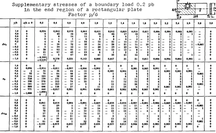
4.1. The supplementary stresses of the unit line load p

=

P!2 c

4.1.1. The state of plate stress

The boundary loads 2 pc according to Section 2.2 must be so arranged in the strip of plate that they reach equilibrium within a length L; the distance between them must also be great enough so that the regions of influence of

their supplementary stresses do not overlap. According to Saint Venant it is

in " = o. M = -

!f

(0ｾ c)= ... = - 0,295_{pb ' •}

fixed at both ends at ±a according to Fig. 3a.

this, with clb

=

0.1 and

approximately at a dista.nce equal to the height of the plate; accordingly a

period L(= 2 a)

=

8

b snould Just barely suffice in order to avoid any mutual

overlapping. This is correct provided extreme demands for accuracy are not

made and an error of about 0.5% can be regarded as acceptable. However, for

our purposes, in order to get the numerical values accurate to three decimal places, for undistorted stress compensation we must work with a load interval

of approximately three times the height of the plate. Accordingly, the period

within which a boundary load group reaches equilibrium has the length L

=

12 b.

Figure 3 shows the loading scheme for stress calculation. As was already

established in Section 3, in order to determine the state of supplementary stress for a given loading, the loaded boundaries can also be interchanged; it does not matter, therefore, whether the line loads 2 pc are applied

alter-nately on the upper and lower boundaries, or only on the lower one. We

choose the latter arrangement (Fig. 3a), because the calculation of the

stress-es according to equation (12) is easier if only one boundary is loaded. The

Fourier coefficient an according to equation

(4)

is given in Fig. 3b. The

stress components are determined point by point in a network, the distance between the nodes of which in the x and y directions is 0.2 b, equal to the

length of the unit load. In order to obtain the numerical values with

cer-tainty to at least three decimal places, it was necessary to take up to 41 series of terms into account in the immediate region of the load.

4.1.2. The elementary state of stress

In the elementary theory of bending the beam

corresponds to a strip of plate of length L

=

2 a

According to the rules of statics, for a rod like

alb

=

6

Q =0; pc

in " ...±c. M ... - 2"(0 - 2 c)= ... = - 0,290pbl •

Q ...±pe= ±0,1pb •

The variation of Q and M over the length L is indicated in Fig. 3 c.

From this the elementary stresses are obtained according to equation 1. With

I

=

ｾ

db for the rectangular cross-sections,

in"=' O. as'=> - i3 Md bl • -;;r '= ...

+

0,44256' •r ""j ,p

-12-4.1.3. The representation of the ｳｵｰｰｬ･ｲｮ･ｮｴ｡ｲｾ stresses

The complete state of supplementary stress for the load P

=

0.2 pb at

x

=

0 on the lower boundary is nO..l obtained by deducting. the elementary

stresses according to 4.1.2 from the plate stresses according to ｾＮｬＮｬＮ The

length of the region of influence of the supplementary stresses is independent

of x, and equals

6

b, or three times the height of the plate (Fig. 3d).

The results could be summarized in a single numerical table. In order to

be able to mUltiply the unit length 0.2 b of the unit load by arbitrary whole numbers as assumed in Section 4, the numerical values at tha intermediate

points for 0.1 b, 0.3 b ... would also have to be stated. Basically, however,

we wish to confine ourselves to stress determinations only at the tenth points of the plate; it is therefore expedient to divide the results into

Tables I and II for load length of 0.2 band 0.4 b. For odd multiples of load

lengths 0.2 b the supplementary stresses are then obtained by superposition of the values of Table I, and for even multiples by superposition of the values

of Table II. The Bupplementary stresses are mirror symmetrical to the y axis,

the tables therefore contain only the rir;ht half of the supplementary stress

field. _{For the left half the values for 60 x and 0y have the same sign, and}

for Ｖｾｸｹ the opposite sign. The sign rules must also be observed for an

interchange of boundaries of application.

With the aid of Tables I and II any arbitrary elementary state of bending stress in an at first still infinitely long rod with given boundary loading

can now be expanded to the statically equivalent state of plate stress. In

order to emphasize the unique importance of the supplementary stresses and also to point up the relationships already dealt with between the elementary theory of bending and the plate theory in still another way, the numerical values of Table I are plotted in sections at right angles to the x axis at

each network point (Fig.

4).

The lines of stress in the in@ediate region of application of the boundary load emphatically show the extremely large changes of stress an elastically isotropic building material is compelled to undergo in a small zone if it is simultaneously to satisfy the geometrical boundary conditions with reference to the neighbouring cross-sections, the static boundary conditions at the

outside, and the equilibrium conditions. In the case of static boundary

conditions it is particularly the discontinuity in the boundary stress a at

y

x = to.l b changing from the full boundary pressure under the load to zero,

which also compels the supplementary stresses ｾｯ to Jump at these points from

x

large negative to positive values. At the transition from the load of finite

length to the point load the stresses are mathematically even infinitely large. Obviously the most elastic of building materials cannot withstand such changes

of ｳｴｉｾｓｓ at certain points without local plastic deformations. To be sure, the stress peaks are thereby weakened and need not be overvalued, but the

first stress lines for 60_x in Fig.

4

indicates to ｾｉｨ｡ｴ extent a brittle

nlaterial such as concrete, for ･ｸ｡ｮｾｬ･Ｌ is exposed to danger of cracking in

the immediate vicinity of concentrated compressive forces.

In

Fig.

5

the lines of contour of equal normal stresses 0y are plotted.

This type of presentation is particularly suitable here for showing the rapidly spreading and fading wave-like effect of a concentrated boundary

discontinuity in a plate. The boundary stresses decrease to less than 2% of

their initial value in an approximately square area bounded by roughly

0.8

times the height of the plate. Contour line charts for the other

supplemen-tary stresses 60x and Ｖｾｸｹ display a similar pattern.

If concentrated boundary loads appear in the determination of a state of plate stress, then for the numerical calculation a finite load length of the substitute line load must be established which agrees as closely as possible

with the true load length. Figure

6

shows that with load length between 0.1

and 0.4 times the height of the plate the supplementary stresses in the

immediate region of the load do indeed differ considerably from each other, the differences, however, decrease with increasing distance from the load just as rapidly as the supplementary stresses themselves.

4.2. The supplementary stresses for other boundary loads

4.2.1. Expanded unit loads and load groups

Use has already been made of an increase of length of the unit load from

0.2 b to 0.4 b in setting up Table II. Two unit loads 0.2 pb are placed side

by side so that they touch at x

=

O. Thus theIr stress components at section

ｾ｢

=

0.1, 0.3, 0.5, which are 0.2 b apart, are superimposed to give those of

the line load 0.4 pb at sections ｾ｢

=

0.2, 0.4, 0.6 Similarly the stress

components of three unit loads situated side by side can be superimposed for

those of a line load of length 0.6 b, etc.

It is also possible now to determine the supplementary stress in a given

area due to a group of loads the lengths of ｾＯｨｩ｣ｨ may be derived from the unit

load length 0.2 b, but whose magnitude, direction, and boundary of

applica-tion are different. For this purpose we make use of the fact that the stress

lines represented in Fig. 4 at section ｾ｢

=

0, 0.2, 0.4 ... owing to a

boundary load 0.2 b at x

=

0, are merely the influence lines of the

supple-mentary stresses at the section x

=

0 for a moving load 0.2 b at the boundary

points ｾ｢

=

0, 0.2, 0.4 ... Since the reference point can be arbitrarily

displaced along both boundaries, the boundary loads of arbitrary length and magnitude applied at various points need only be nrultiplied by the ordinates

-ll.J--of their corresponding influence lines, and the results superimposed. The

application of this principle will be illustrated below by a numerical example. 4.2.2. The supplementary stresses of the uniformly distributed load p

In a strip of plate uniformly subjected over its entire lenGth to a load

p, all sections at right angles to the plate axis are the same with respect to

the supplementary stresses independent of x. In the course of deformation the

sections must all remain plane, since each section is also the plane of

sym-metry for the adjacent sections. The cross-sections would become curved owing

to one-sided boundary loading, unless they were othe rwf.ae prevented from doing

so. Besides supplementary stresses 0y(p), therefore, equilibriwn systems

60x(p) must also ｯ｣｣ｵｲｾ and must also be the same in all sections.

Supplemen-tary stresses ＶｾｘｙＨｐＩＬ however, do not occur.

The numerical values for 1'.::.0_x(p) and

°

_y(p) can also be determined

accord-ing to ll.2.1 from the stress lines of the unit load. As was done in Fig. 4

for cross-sections, we can imagine the supplementary stress components of the

unit load plotted in longitudinal sections at right angles to the y axis.

These again may be regarded as influence lines. At x -

±3

b they reduce to

zero; their halves which are mirror symmetrical about x

=

0 have the same sign

for 60x and 0y' and opposite sign for ｾｾｸｹＮ In order to obtain the

supplemen-tary stress ordinate for p at the height ｹｾ the area enclosed at this height

by the influence line can be numerically integrated. Other solutions are

known from the literature for this special case, which is simple to deal with

analytically. For example, Worch(2), by dividing Airy's stress function into

a fundamental and a supplementary function for the case of uniform load, found mathematically closed expressions for the partial functions, from which the

supplementary stresses can then be derived by differentiation. The two

calculations were carried out and compared. Agreement is practically total.

The result is plotted in Fig.

7.

5.

The Supplementary Stresses in the Plate of Finite Length

We have been considering the infinitely long plate subject to bending stress, in which after separation of the elementary state of bending stress only the states of equilibrium of the already known supplementary stresses

remained. If we cut through the plate at an arbitrary point the section

forces present there must be eliminated by superposition of the external

forces of inversely equal magnitude in order to satisfy the new geometric con-ditions of an end boundary that has now been bared; this can involve

supple-mentary stresses 60_x or ｾｾ _xy, or both sirnultaneously. The section boundary

can, however, be free of forces, prOVided the nearest boundary load is 1.5

lower accuracy, at least 1.0 times the height of the plate. In such a case the principles for calculating states of plate stress in the rod of infinite

length, as developed in Section

4,

can also apply to the plate with three or

four boundaries in the finite region.

The equilibrium system of the inverse supplementary stresses to be

applied at the section boundary now not only causes these stresses to vanish, but produces an additional supplementary state of stress to be superimposed on one already present from the boundary loads, and according to Saint Venant reduces to zero at a distance from the boundary approximately equal to the

height of the plate. The influence of this intrinsic boundary load can be

taken into account by a procedure(5) which the author has already used several

times in the solution of plate problems(6-8). The method shows a solution for

the square plate where three boundaries are free of forces and the fourth is SUbject to an intrinsic load, i.e. it satisfies precisely the conditions for the end boundary of a sliced rectangular plate to be made force free.

Unlike the case of the infinitely long plate, where a single solution for a unit boundary load suffices for the treatment of all other types of boundary

load, the supplementary state of plate stress must always be determined separately for the section correction force at the end boundary depending on

the length and position of the boundary load in question. Even here, however,

certain simplifications are possible if correction stress states are procured for unit loads moving along the boundary which can be superimposed as reqUired. Here we shall confine ourselves to the investigation of the two most important cases, namely a unit line load 0.2 pb applied to the end of the rod, and the correction in the supplementary stresses of the equivalent load p, which needs

to be carried out only once. The effect of a single load at the end of the

rod is required for the determination of plate states of stress at the ends of freely supported or continuous beams for a given boun"dary load; the known possibilities for an exact stress calculation are thus expanded.

5.1. The supplementary stresses for a unit line load at the end of the beam The section shOUld be cut through the plate in such a way that only one

liberated ｳｴｾｴ･ of stress has to be eliminated by superposition, e.g. if the

section plane is also a plane of symmetry for the boundary loading of the

plate, then only supplementary stress ｾｯｸ remain, and the ｾｾｸｹ stresses vanish.

The initial system for the end of the plate with line load 0.2 b is

accordingly the strip of plate already known from Table II with the line load

0.4 pb, which is sliced through in the centre of the load at x

=

o.

Figure 8 shows how the intrinsic stress ｾ｡ｸ taken from Table II must be

treated along the section boundary in order to obtain from it the ｳｵｰｰｬ･ｮｾｮﾭ

-16-load must be approximated by rectangular partial loaels, because only foT' these

are table values available for stress dc t.e rnu.natLon . The aubst tt.u t.e load

obtained in this manner must, however, satisfy the same conditions as the

initial load: as intrinsic load they must not have any resultant force nor

any moment, and moreover the boundary stress

° (.;;

=

0) determined from it

x

according to ref. 5 must coincide as closely as possible with the initial

stress tJ.o. The two former conditions are satisfied \'Ii th the equilibrium test

x

given in the table accompan ying Fie;. [3, and the boundary stress 0y (.;; :::: 0)

(broken line curve in Fig. 8) coincides almost ｣ｯｮｾｬ･ｴ･ｬｹ hith the initial

load.

It may come as a surprise that the rectangular approximate load, although

it apparently approximates the initial load so roughly, can nevertheless

pro-duce a closely agreeing boundary stress. It must be remembered, however , that

even a discontinuously variable load, as the result of a trigonometric series,

can also yield a continuously varying boundary stress. It is only necessary,

therefore, to choose the rectangular partial loads in number and form as

simply as possible and fit them into the tabular values(5), in order to reduce

the Vlork of calculation to a minimum. The best way is to proceed by first

determining the content of a partial area of the stress fic;ure tJ.0_x according

to ｓｩｮｾｳｯｮＧｳ rUle, establishing a rectangular substitute load for this and

supplementing the latter with the remaining partial loads while bearing the

two equilibrium conditions in mind. The boundary stresses 0x(';; :::: 0)

corre-sponding to this load are then determined and compared for their agreement

with the initial stress tJ.o. As a rule a first, or even a second correction

x

of the substitute load will be necessary, but after some practice this is done

qu LckIy , However, even when a certain residual state remains from the

differ-ence between tJ.o and

° (.;;

=

0) this is of no practical importance. This

x x

residual state is also a state of intrinsic stress without resultant, ｾｬｩ｣ｨ

disappears rapidly towards the interior of the plate.

The state of stress correction in the end squares due to tJ.0

x at the

section boundary cannot be determined with the same accuracy as its initial

state On the strip of plate as given in Table II, the values obtained by

superposition in Table III are therefore given only to three decimal places.

In Fig. 9 the numerical values of 'I'ab Le III are plotted in cross-sections

as those of Table I were in Fig. 4. The comparison with the stress line of

the supplementary stresses in the interior of the strip of plate given in

Fig.

4

shows to what an extent just the new conditions at the section boundary

now liberated have changed the oric;inal course of the three supplementary stresses far into the interior of the plate, although the static boundary conditions on the long side and the equilibrium conditiW1S have remained the

sarrle. The strong increase of boundary tensile stresses 60

x near the load is

particularly striking. This merely ｣ｯｮｦｩｾｬｳ the fact that the danger of

cracks beginning at the boundary and going inward 1s particularly great near concentrated loads, e.g. at the end supports of beams or near brackets with

individual loads at the end. Moreover, since the external moments here are

zero, Navier's theory of bending does not by itself suffice to assess the stress in the material.

5.2. The supplementary stresses of the static load p at ｴｾ･ end of the beam

In the infinitely long plate with uniform loading of one boundary

accord-ing to Fig. 7, the system of equilibrium 60_x(p) is used in order to ensure

each individual cross-section remaining plane as required for reasons of

symmetry. If the plate is sliced through at an arbitrary point, the exposed

boundary, owing to the vanishing of the section forces 60_x(p) must ｢･｣ｯｲｲｾ

arched. In order to prevent this we proceed in the same manner as in

Section 5.1 with the treatment of the unit line load. By reason of the

bound-ary stress 60_x(p) applied at the section boundary, an additional state of

supplementary stress is produced in the square compensation region, a state

which is superimposed on the one already present. Table IV and Fig. 10 show

the result. The new supplementary stresses 60 (p) now increase continuously_x

from zero up to their full value in the strip of plate no longer distorted

by the section at x = 2 b. Simultaneously with the possible arching of the

section boundary owing to p, a new system of equilibrium of shearing stresses,

which is of course unimportant, arises. The supplementary stresses 0y(p) are

but little affected by the cutting.

6.

The Practical Application of the Method

The examples are so chosen that the practical importance of the method and the scope of its application can be shown as comprehensively as possible. Wherever there is a possibility of doing so, plate problems for which

solu-tions by other methods are already known are dealt ｾｊｩｴｨＮ

6.1. State of stress in the infinitely lonG plate

Example 1 (Figure 11)

The plate with two opposite single loads

This simplest case of a complete state of plate stress is one of the classic ones in plate literature, and the problem has been solved amongst others by Filon(3), section 35 for individual point loads with the aid of

Fourier integrals. The probleln has practical significance, for example, if a

-18-directly below it, or if the narrow flange of a continuous pre-stressed concrete beam is vertically pre-stressed locally in the region of the inside support in order to reduce excessively high skew principal tensile stresses.

Since there is no elementary state of bending stress here, only

supplementary stresse8 in the sense of Section 3 occur. Let the length of

loading be one-tenth the height of the beam. For this the stress conwonents

can be taken directly from Table I, and the numerical values need only be

superimposed by their mirror values relative to the x axis. For the sections

ｾ｢

=

0 and 0.1 the total stresses are given in tabular form in Fig. 11, and

a few characteristic lines of stress are plotted. The principal tensile

stresses are then calculated in a known manner from stress components 6o

x' 0y

and Ｖｾｸｹ and are plotted in Fig. 12 at the one-tenth points of the upper half

according to magnitude and direction. In the lower half they are drawn as

lines of contour. The last third of the region of compensation between 2.0

and 3.0 b has been left out, since the stress magnitUdes here are negligible. The pattern of principal stresses here" again confirms the fact, already

pointed out several times (e.g. in references

5

and

8),

that the absorption of

the tensile stresses between the loads is not the only measure reqUired for

the prevention of cracking. Wherever concentrated compressive forces occur at

plate boundaries the boundary tensile stresses on both sides of the points of application are almost always greater than the simultaneous tensile stresses

between them. Protection of the boundary close to the load against cracking

thus becomes particularly important, even when no moment or transverse forces

have to be taken into account as well. Figure 12 shows clearly that the

correct direction of the reinforcement in such a case must be a horizontal reinforcement distributed more or less uniformly over the height of the crOSB-section, which can be anchored in the adjacent compression zone on both sides and also a tensile reinforcement which must be deflected downwards into the area behind the pressure zone.

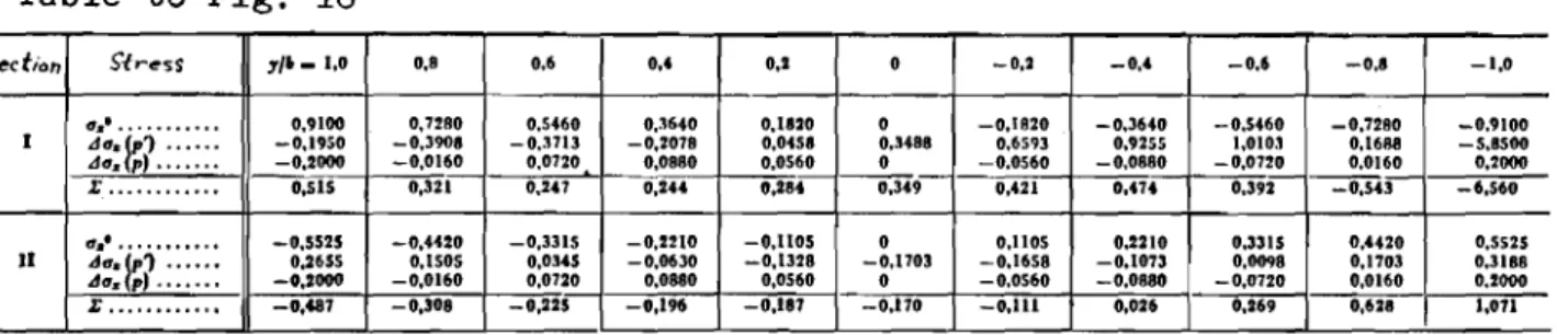
Example 2 (Figure 13)

The ｾｴｲｩｰ of plate with two single loads not opposite each other

The lines of shearing stress at sections I and II must be determined for

various eccentricities e. This problem has already been dealt with earlier

for individual point loads, amongst others by Filon, Seewald(l) and Girkmann ( 3 ) .

(a) The elementary state of stress

The rod, supported at infinity, is kept in equilibrium by the moment 2 Pe; apart from the load application on both sides, therefore, the plate is

free of transverse force. OWing to the variation of transverse force, in

cross-section we have

in section I - I

T%II(O) =0

in section II - II

T%II(O)=

Ｍｾｾ｛ｉＭＨｦｲｊ］ｾ｛ｉＭＨｾｲｬｾ

(b) The state of tensile stress

The influence values for the line load 0.2 pb are again taken from

Table I. In accordance with the rule of signs of the shearing stresses for

section I - I the negative numerical values of Ｖｾｸｹ at x

=

3

e are to be

superimposed with the mirror positive values at x

=

e, and for the section

II - II the negative values at x

=

e are to be superimposed ,11th their own

mirrored negative values.

In the table to Fig. 13 the total stresses are calculated by tabulation;

in each case the first of the three nwnbers of a network point applies to the elementary stress, the second to the tensile stress of the load at the lower

boundary and the third for that of the load of the upper boundary. The shape

of the shearing stress curve plotted in Fig. 13a is typical (c r , Fig. ｌｾＲ in

ref. 3). The shorter the distance between the loads (section II - II), the

more the shearing stress peaks are displaced towards the boundary: the

familiar parabolic distribution in the section II - II is not attained until the loads have moved sufficiently apart so that their supplementary stresses no longer overlap; this is already more or less the case according to Table I

at e/b

=

0.8. Outside the loads (section I - I), in the region free of

trans-verse forces, the shearing stresses, to be sure, only form pure equilibrium states, but their maximum values are nevertheless of the same order of

magnitude as in section II - II. Example 3 (Figure 14)

The strip of plate with shear loading

When, as shown in Fig. 13, two loads come so close together that the section perpendicular to the rod axis touches both, we then have the so-called

shearing load case. Let us determine the complete principal stress pattern

for this case, but with twice the length of line load as in Example 2. (a) The elementary state of stress

The infinitely long rod is kept in equilibrium by the moment 2 Pe

=

0.16 pb:2. From the shape of the shears and moments given in Fig. 14b it

follows according to equation (1) that

in" ... 0,

"_ 3 Q[

(")"1

31

("I)"1

P

-20-TzVO= ...

］ｾ｛ｉＭＨｾｮｾ［

inxlb =0,4. uz o= '" = 0,1200

f .

ｾＬ

T Z lIo=O.

(b) The state of supplementary stresses

The influence values of the line loads 0.4 pb can be obtained from

Table II. Basically the same numerical calculation procedure is followed as

in Example 2, so that only a few stress components need be ｳｨｯＬｾｮ in the table

to Fig. 14. In Fig. 14a the most important stress lines are plotted. Whereas

in Example 1 the a_x shape was determined only by supplementary stresses ｾｯ _x,

here slight elementary bending stresses have arisen also, due to the

displace-ment modisplace-ment. These however, have not affected the original curve appreciably.

The ｾｸｹ curve has already been described in Example 2. The principal tensile

stresses have also been determined and are plotted in Fig. 15 for the region

of the plate bounded by x

=

0 and +2 b. In the region x

=

±2 b the

supplemen-tary stresses have already faded to such an extent that the general pattern is rapidly approaching that of the purely elementary state of bending stress

owing to M= 0.08 pb2

•

Comparison with the principal stress diagram 12 of the first example clearly shows what the effect has been of displacing the line loads, which were originally exactly opposite each other, in opposite directions to form

the pure shearing case. In Exarrwle 3, of course, the load length is twice

as great as in Example 1, but this does not affect the basic results. Owing

to the stabilization moment that has now been added, the principal tensile stresses are increased on one side and decreased correspondingly on the other.

side. As a consequence the interior compression zone, originally situated

centrally for reasons of ｳｾｮ･ｴｲｹＬ has moved towards the bending compression

side and has combined with the second compression zone in the region of

initiation of the boundary load. The added transverse force, moreover, has

resulted in a considerable increase in the principal tensile stresses. Example 4 (Figure 16)

Internal field of a continuous diaphravn beam

This is the plate problem as dealt with by Bay, Craemer, Dischinger,

Timpe and others. So that the support pressures will all be equal and thus

independent of changes of form in the plate, the beam must be very long and

the bay length always the same. In addition the loading within a period

length L (see Section 2.1) must be ｳｹｮｭｾｴｲｩ｣｡ｬ or antisymmetrical to x

=

0,

L, 2L ... The problem has also been dealt with in detail in reference 3 and

finally Thon(9) has still further expanded the partial results, hitherto known only for uniform loading.

let the ins ide bay have a length

:>

b , Let the oeD.rinc:: ｊ･ｮ｛ｾｴｨ be 0.11 b.

Here we a gaIn show the calculation scheme which is a Jvrays t.he sarue , but in

this case we confine ourselves to the deter-nu.nat.Lon of the no rmaI stresses

°

_x over the support and in the centre of the bay.

(a) The elementary state of stress

For a rod loaded according to Fig. 1Gb, it is generally true that with

L c

x

=

2b and P == b

in section I

-

I M = - pb'6 (2 ,,' - 3"e+e'),

pb' (16)

in section II

-

II M = ""6('" - e")·

For x =

2-

and p = 1 then

5'

2 in section I

-

I M = - p b"ｕｾ

_

ｾ +ｾＩ = _ 3M Pb" 6 4 10 25 600 ' in section II

-

II M =pb'

(!

｟ｾＩ = 221 pb ' 6 ." 25 600 •

From this with I == ｾ db3 _{for the rectangular cross-section the elementary}

bending stresses according to equation (1) are obtained as in in section I - I uz"= - "2 .3 db" . bM y =0,9100 b . d 'y p

in section II - II u","= ... = - 0,5525

f .

ｾＮ

(b) The state of supplementary stress

The uniform load p at the top and the line load pi at the bottom

according to Fig. l6a must be taken into account. The influence values ｾ｡ｸ

for p, equal in all sections, can be obtained directly froIn the table ｩｾ

Fig. 7, while those for 0.4 p Ib

=

ｾ

(o.«

pb ) are obtained from Table II and

mUltiplied by

7.5.

At the same time for the section

I - I

the positive values

ｾｯｸ of Table I I for ｾ｢ = 0 and ｾ｢ == 3.0 must be superimposed, and for

section II - II the positive values for ｾ｢ == 1.5 are to be doubled. The

latter are not contained in Table II, but With good approximation the mean

values between 1.4 and 1.6 can be used in place of them.

The stress components in the table to Fig. 16 have been determined in the

same way as in the previous example and represented in Fig. 16a. Agreement

with the corresponding numerical values obtained according to the usual methods of the plate theory, e.g. by Dischinger (Girkmann(3)), only after

time-consuming calculations, is complete. Only the 60_x values in the section II - II

are not quite accurate, because the influence values for So_x when ｾ｢ == 1.5

were determined for the sake of simplicity between the values at ｾ｢ == ＱＮｌｾ and

L c 1

x ; 2 b

=

10 and p

=

b

=

5

as in

at x = 0 (centre of support)

ＭＲｾＭ

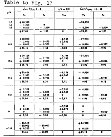
Example 5 (Figure 17)

Inside bay of a continuous slender beam

Let the static system of the girder and its loading be the same as for

the continuous diaphragm beam 1n Example Ll, but let the slenderness be that of

a common beam, namely L/2 b = 10. The bearing distance remains ｏＮｌｾ b,

cor-responding approximately to the true conditions with one-fifth the heieht of

the girder. We wish to determine to what extent the results of the elementary

theory of bending and the plate theory differ from each other in the distor-tion region of the support load and in the centre of the bay.

The calculation procedure is the same as in Example it, except that the

numerical ratio of the elementary stresses to the supplementary stresses is

different. To determine the principal stresses the shear and moments in the

distortion region of the support load (hatched area in Fig. 17a) must be fully

known. This region is shown enlarged in Fig. 17c.

(a) The elementary state of stress For the rod in Fig. 17b first with

Example 4, we have in the section I - I

p

b'

p

b'(

1)

M = ｾ - -(2 ,,' - 3 "e+e')= - - 200 - 6

+-6 6 25

= - 32,Hpb" ,

in the section II - II at ｾ｢ = 10 (centre of bay)

pb' pb' (

1)

M = 6 (,," - II")= 6 100 - 25 = 16,66 pb'.

The pattern of shear in the region of' influence of the support force

0.4 p'b is plotted in Fig. 17d. The elementary stresses are then obtained

from this again according to equation (1). (b) The state of supplementary stress

The same remarks hold as for Example 4, where the influence length of

the support load extends over only a fraction of the bay length.

The calculation procedure is shown in the table to Fig. 17 for a number

of stress components. Vales are given for ax and 0y at the centre of the

support (section I - I) and at midspan (section II - II) and for ｾ _xy at x

=

0.2 b directly beside the support. vfuereas at the centre of the bay the

dif-ference between the elementary rectilinear and the true course of the normal stresses is practically negligible, this is not so in the cross-section above

the support. In Fig. 18, therefore, the principal stresses in the influence

region of the support load as obtained according to the elementary theory of

bending and according to the plate theory, are compared with each other. We

have again omitted the representation in the last third between 2.0 band 3.0 b, since the differences no longer play any part on account of the preponderant influence of the elementary stresses.

The comparison of the principal stresses in Fig. 18 confirms the known fact that the compressive stresses at right angles to the rod axis in the imnediate region of load application of the support in reality admit no

principal tensile stresses(lO). As a consequence the resultant principal

tensile force experiences not only one more initial deflection towards the horizontal and hence a shift away from the support, but also a certain reduc-tion in its absolute value.

6.2. State of stress in the end region of a rectangular plate Example 6 (Figure 19)

The end of the plate with two individual loads opposite each other

As in the case of Example 1, there is no elementary state of bending

stress here, and thus only the influence values of Table I I I are to be

super-imposed with their values mirror symmetrical to the x axis. The development

of the Ox stresses from the section boundary to the interior of the plate is

indicated in Fig. 19a for a few cross-sections. The principal stresses are

plotted in Fig. 20, again with their stress component in scale with respect to magnitude and direction in the upper half, and as lines of contour in the

lower half. Comparison with Fig. 12 shows the effect of slicing the plate

through the centre of the line load 0.4 pb. The tensile force between the

loads which has held the two separating halves together has vanished as a

result of the slicing. As a ｣ｯｮｳ･ｱｾ･ｮ｣･ the compression zone in the interior

has extended and shifted towards the end boundary and has merged with the second, only slightly extended, but much more intensive compression zone in the load initiation region.

Of practical interest in both cases is the maximum tensile force in the

direction of the rod axis which occurs as a consequence of the concentrated

boundary loading. In the strip of plate we are concerned with the tensile

force between the loads and boundary tensile forces, and in the sliced plate

only with boundary tensile forces. The two cases are represented in Fig. 19b.

The tensile force between the loads and the boundary tensile force are approximately equal to the interior of the plate, but the boundary tensile force at the end of the plate is about five times greater.

Example 7 (Figure 21)

The simply supported diaphragm beam with a single load

The distribution of normal stresses a is to be determined at the

x

centre of the bay for the cases where the line load 0.4 pb is initiated from

above as pressure and from below as tensile force. With the chosen aspect

ratio 4/2 b

=

2.1 it is still Just possible to employ Table I I for the state

according to

::: 2 db3

3

-21+-accordance with Section 5.1 there is still a system of equilibrium

supplemen-tary stresses 6o

x' with the overlapping of two states of supplementary stress,

synunetrical to the plane of the section along the section boundaries x ::: ±2 b,

but this correction. according to ref.

5.

has just faded to zero by the time

it reaches the centre of the girder. (a) The elementary state of stress

At midspan M ::: 0.2 pb2 ( 2 . 0 _{- 0.1) ::: 0.38 pb}2

• From this,

equation (1), we have for the rectangular cross-section with I

3 M y y p

0,,° = - '2 .db' ' b = - 0,57b .d .

(b) The state of supplementary stress

For bearing pressures 0.2 pb take twice the positive numerical values of

Table III for ｾ｢ ::: 2.0j for the load 0.4 pb initiated from above

compres-sively, the positive values 60x(0) of Table II are to be mirrored and for the load initiated from below with tensile force we may take the same numerical values with opposite sign.

The results are calculated in the table to Fig. 21.

Example 8 (Figure 22)

The wall-like girder with cantilever arms

Let a plate with aspect ratio ｾＲ b ::: 1+ be supported at two points one

quarter of its length from the ends. We shall determine the pattern of

principal stresses for a uniform load p at the upper boundary. (a) The state of elementary stress

From the curve of shear in Fig. 22b it follows, according to equation (1) that in section I in section II 0,,0= T".,O= 0 3 M y y p 0,,°= - 2dbl •b= .. , = 2.970-,; •d T".,O= 0

(b) The state of supplementary stress

For the supplementary stresses, from the uniform load p, Table IV holds

in the square end region (see also Fig. 10). The maximum value at 2.0 b then

continues unchanged into the interior (see Fig. 7). For the supplementary

stresses of the line loads 0.4 plb Table II applies directly at first only in

the region of the inside bay. For the cantilever arm region we proceed as

follows: Imagine the cantilever beam of length L continued on both sides in

the same pattern. The influence values of two neighbouring line loads then

separation in section IV is reconstructed, a system of equilibrium normal

stresses ｾｯ _x remains, which must be eliminated in accordance with Section 5.1

by superposition. No shearing stresses ｾｾｘｹ occur in section IV.

In order to illustrate the calculation procedure here, a number of stress

components are determined in the table to Fig. 22 in the already known manner. For sections I and II the stresses are final, for section III a slight addi-tional improvement is obtained from superposition of the correction· stress

ｾｏｸ in section IV applied to a square area. We shall not deal further here

with this correction calculation in accordance with Section 5.1 and Fig.

8.

Figure 23 shows the principal stresses resulting from the total state of

stress for ax, 0y and ｾｸｹ taking into account the improvement in accordance

with Section 5.1. The figure also gives an idea of the bearing behaviour of

diaphragm brackets. Even though no generalization of the solution to this is

possible, because the boundary conditions, especially at the support section, differ from case to case, nevertheless a method of rigorous treatment of this important problem has been illustrated which can also be adopted in many

similar cases. Other boundary conditions in the support and in the load

initiation region influence the total state of stress in a different manner.

In an earlier paper(7) the author has already investigated another type of

load initiation along the end boundary showing the effect on square brackets with individual loads at the end of the bracket of a displacelnent of the point

of load application in the direction of the force. Even so, however, the

complex problem of short brackets is still not adequately solved. Especially

brackets within the range of a/2 b < 1 (see Fig. 2) with their complex state

of stress, and with the elementary stresses continuously diminishing in

comparison with the supplementary stresses must be further clarified, but this will be reserved for a later investigation.

7. The Statically Indeterminately Supported DiaEhragm Beam

The above examples all assume definite boundary loads. Even in

Examples

4

and

5

the support pressures on the continuous girders were all of

equal magnitude, for reasons of structural and load SYmmetry, and hence were

pre-determined. However, in all cases where the support pressures are not

determined solely by eqUilibrium conditions, but also depend on the deforma-tion behaviour of the structure, difficulties arise in applying the method. Consideration of a continuous beam on rigid supports according to the normal rules of rod statistics no longer suffices to determine the elementary state

of stress. In the elementary theory of bending the geometric boundary

condi-tions of vertical undisplacibility of the supported boundary points is always referred, by implication, to the axis of the rod, but in a compact plate the

-26-other deformations are no longer negligible compared with the bending of the

rod axis. Here it is particularly the elastic compression between the loaded

boundary and the axis of the rod which influences the distribution of sectional forces.

The problem has been dealt with for the diaphragm over two equal bays

by Parkus(ll) and for the two-bay and three-bay beams by Bay(12). Parkus

investigated the beam with continuous uniform load and with uniform load by bays, basing the procedure for the solution on Girkmann's general solution for the single bay(3) with the aid of Fourier series; the mathematical work

involved in this is considerable. Bay also obtained sufficiently accurate

results for continuous uniform load with the aid of differential calculation in a somewhat simpler manner.

According to the method described here, however, no restriction is

placed on the calculation of states of stress in the plate in continuous beams with statically indeterminate supports, if the geometrical boundary condition

at the bearing points v

y

=

0 can be introduced into the rod system for

deter-mination of the elementary state of bending stress in such a way that the

correction distribution of sectional forces is obtained. The beam on rigid

supports becomes a beam on elastically compressible supports, the coefficient of elasticity of the supports being a correction which must be applied to the beam on rigid supports in order to obtain the distribution of sectional forces

corresponding to the true deformation of the plate. This does not affect the

treatment of the state of supplementary stress in any way. 8. Summary

Any state of stress in a plate satisf¥1ng Airy's stress function can be

divided into an elementary state of Ｘｴｲ･ｳｾ and a state of supplementary stress.

The state of elementary stress

knRwn

from ｴｨｾ pasic theory of bending already

satisfies the equilibrium condit+ons, while ｾｨ･ state of supplementary stress

in the sections perpendicular to the axis of the rod merely represents a cor-rection of the stress curve without a resultant of its own, which does not

influence the sectional forces in the direction of the rod axis. Thus states

of stress in the plate can also be composed of elementary stresses and sup-plementary stresses, the elementary stresses having to be determined from case to case by the usual rules of rod statics, while the supplementary stresses

need only be determined once for each kind of load. The influence values of

the supplementary stresses are given for the most important boundary condi-tions, and the simple and rapid application of the method is demonstrated for

a number of examples. The method is applicable even to continuous plates

conditions in the plate compared with the slender rod are taken into account in determining the state of elementary stress by means of supplementary support conditions.

References 1.

2.

"

Seewald, F. Die Spannungen und Formanderungen von Ba1ken mit

rechteckigem Querschnitt. Abh. a. d. Aerodyn. Inst. a. d. Techn.

Hochsch. Aachen, (7), 1927.

n, "

Worch, G. uoer Zusammenhange zwischen del' technischen Ba1kenbiege1ehre

und del' Scheibentheorie. Bautechnik-Arch1v, (5): 43, 1949;

Wilhelm Ernst and Sohn, Berlin.

Worch, G. E1astische Scheiben.

3.

4.

Girkmann, K. F1achentragwerke.

"

5.Auf1.Wien. Springer-Verlag 1959.

Beton-Ka1ender 1956.

5. Sch1eeh, W. Die Rechteckscheibe mit be1iebiger Be1aatung del' kurzen

Randel'. B.u.St. (3): 72, 1961.

6.

7.

8.

9.

10. 11.

"

Sch1eeh, W. Die Zwangspannungen in einseitig festgeha1tenen Wandacheiben.

s.u.se.

(3): 64, 1962.

Sch1eeh, W. Del' Spannungszustand in del' Kragscheibe mit Einze11ast.

Bautechnik, (7): 240, 1962.

Sch1eeh, W. Die SpannungszustHnde beim AUf1ager einea SpannbetontrHgera.

B.u.St. (7): 157, 1963.

Thon, R. Beitrag zur Berechnung und Bemesaung durch1aufender wandartiger

TrHger. B.u.St. (12): 297, 1958.

Bay, H. Die achiefen Hauptzugapannungen beim Eiaenbetonba1ken.

logenieur-Archiv, 4: 244, 1933.

Parkus, H. Del' wandartige TrHger auf drei StUtzen. BaterI'. log.-Arch.

(2): 186, 1948.

12. Bay, H. Wandartiger TrHger und Bogenacheibe. Verlag Konrad Wittwer