HAL Id: hal-02950606
https://hal.inrae.fr/hal-02950606
Submitted on 27 Nov 2020
HAL is a multi-disciplinary open access
archive for the deposit and dissemination of sci-entific research documents, whether they are pub-lished or not. The documents may come from teaching and research institutions in France or abroad, or from public or private research centers.
L’archive ouverte pluridisciplinaire HAL, est destinée au dépôt et à la diffusion de documents scientifiques de niveau recherche, publiés ou non, émanant des établissements d’enseignement et de recherche français ou étrangers, des laboratoires publics ou privés.
Two decades of research with the GreenLab model in
Agronomy
Philippe de Reffye, Baogang Hu, Mengzhen Kang, Véronique Letort, Marc
Jaeger
To cite this version:
Philippe de Reffye, Baogang Hu, Mengzhen Kang, Véronique Letort, Marc Jaeger. Two decades of research with the GreenLab model in Agronomy. Annals of Botany, Oxford University Press (OUP), 2021, 127 (3), pp.281-295. �10.1093/aob/mcaa172�. �hal-02950606�
Accepted Manuscript
© The Author(s) 2020. Published by Oxford University Press on behalf of the Annals of
Botany Company. All rights reserved. For permissions, please e-mail:
[email protected].
Two decades of research with the GreenLab model in Agronomy
Philippe de REFFYE1,5, Baogang HU2, Mengzhen KANG3, Véronique LETORT4, Marc JAEGER1,5
1
AMAP, Univ Montpellier, CIRAD, CNRS, INRA, IRD, Montpellier, France; 2Chinese Academy of
Sciences, Institute of Automation, National Laboratory of Pattern Recognition (CASIA-NLPR), Beijing, China; 3Chinese Academy of Sciences, Institute of Automation, Key Laboratory of Management and
Control for Complex Systems (CASIA-LMCCS), Beijing, China; 4 CentraleSupelec MICS, Paris-Saclay,
France; 5CIRAD, UMR AMAP, F-34398 Montpellier, France
* For correspondence. E-mail [email protected]
Accepted Manuscript
2
Background With up to two hundred published contributions, the GreenLab
mathematical model of plant growth developed since 2000 under Sino-French
cooperation for agronomic applications, is descended from the structural models
developed in the AMAP unit (de Reffye, 1988) that characterize the development of
plants and encompass them in a conceptual mathematical framework. The model also
incorporates widely recognized crop model concepts (thermal time, light use
efficiency, light interception), adapting them to the level of the individual plant.
Scope Such long-term research work calls for an overview at some point. That is the
objective of this review paper, which retraces the main history of the model’s
development and its current status, highlighting three aspects: (i) What are the key
features of the GreenLab model? (ii) How can the model be a guide for defining
relevant measurement strategies and experimental protocols? (iii) What kind of
applications can such a model address? This last question is answered using case
studies as illustrations, and through the discussion.
Conclusions The results obtained over several decades illustrate a key feature of the
GreenLab model: owing to its concise mathematical formulation based on the
factorization of plant structure, it comes along with dedicated methods and
experimental protocols for its parameter estimation, in the deterministic or stochastic
cases, at single plant or population levels. Besides providing a reliable statistical
framework, this intense and long-term research effort has provided new insights into
the internal trophic regulations of many plant species and new guidelines for genetic
improvement or optimization of crop systems.
Key words: FSPM, stochastic functional structural plant model, organic series, organ cohorts, source
and sink organs.
Accepted Manuscript
3
INTRODUCTION
We present an overview of two decades of developing the GreenLab model and its applications in agronomy. This model inherits both from architectural models, designed to address botany issues, and from crop models, designed to address agronomy issues.
The architectural models of trees (Halle et al., 1978) identify the basic components of tree development. Architectural models and their reiterations rely on a few key notions such as axis types, with monopodial or sympodial ramifications, and axial or terminal flowering. A fundamental model assumption is that the same types of axes are duplicated in the plant at different development stages. This enabled efficient sampling strategies for measurements, paving the way for the calibration and evaluation of models representing the stochastic functioning of meristems.
GreenLab is also affiliated to crop models such as STICS (Brisson et al., 1998), APSIM (Keating et al., 2003), Tomsim (Heuvelink, 1998), Pilote (Maillol et al., 2011), EcoMeristem (Luquet et al., 2006), and SUNFLO (Casadebaig et al., 2011). Some of these models have shown good performances for yield prediction. Most of them share a common set of assumptions: (i) they use stand-level data, such as the leaf area or biomass per organ compartments; (ii) Beer-Lambert's law models light interception by foliage as a function of the leaf area index; (iii) a harvest index, the percentage of biomass allocated to the organ of interest, characterizes the plant or stand yield; (iv) they may incorporate (sub)models, especially for the photosynthesis process, respiration, or for the effect of irrigation, nitrogen, etc. In contrast, crop models have limitations related to the fact that organs are not individualized but pooled into compartments: (i) the initial effect of the seed reserves cannot be represented; (ii) LAI is not easily simulated; (iii) planting density is often ignored; (iv) mortality during development is difficult to integrate; (v) different modules of crop models do not synchronize easily, and their interactions are difficult to model; (vi) variability within the stand is ignored; (vii) for woody plants, girth growth is ignored; (viii) 3D plant representation is not simulated.
Accepted Manuscript
4
Functional-structural plant models (FSPM) combine both structural and functional approaches. FSPMs seek to accurately simulate the physiological functioning associated with plant growth and architecture in relation to environmental parameters. Different formalisms have been proposed for the development modules: object-oriented ones (Eschenbach, 2005), or the most widespread ones which are language-based using L-system grammar (Prusinkiewicz et al., 1988) and its extensions such as XL (Kniemeyer, 2004, Henke et al., 2016) or L-Py (Boudon et al., 2012). The organs play a functional role as source and sink, as shown in Lignum (Perttunen et al.,1998), Vica (Wernecke et al., 2000), L-peach (Allen et al., 2005), and L-Kiwi (Cieslak et al., 2011). They provide interesting insights into plant functioning and a way of integrating the existing biological knowledge of a given plant species. However, the simulations are computationally costly, and their complexity raises difficulties for a rigorous application of statistical methods for parameter estimation and model evaluation based on experimental measurements. Above all, FSPMs concern individual plants: unlike crop models, they do not readily extend to stand scale. In the following, we show that a different modelling strategy can be adopted, as is the case for the GreenLab model, addressing the scientific problem as:
Can we find a concise mathematical representation for metabolic processes with phytomer-level structures to generically describe plant growth and development at an individual phytomer-level up to a stand scale?
We recall here the choices that have governed the choices of equations and formalisms in the GreenLab model, and we summarize two decades of research with GreenLab in plant architecture development and production. The characteristics of GreenLab are:
The GreenLab model is a Functional Structural Plant Model (Sievänen et al., 2014) integrating both functional and structural descriptions for metabolic (or physiological) processes with phytomer-level structures. It enables studies from the organ level up to the macroscopic scale. The plant types studied cover a broad spectrum from herbaceous to trees. It benefits from the
Accepted Manuscript
5
ecophysiological concepts assumed in crop models (thermal time, light or water use efficiency, common pool). The restrictions mentioned for FSPM also apply for GreenLab; the studied stand must be composed of a fixed genotype (clone, variety), with plants of the same age, cultivated in an isotropic environment (e.g. no asymmetric gravitropism or phototropism). Many cultivated plants meet these requirements.
GreenLab is a stochastic, discrete, dynamic mathematical model with a voluntarily limited set of variables and physically interpretable parameters, allowing:
• Parameter estimation (strategy of protocols for data acquisition and inverse methods)
• Model analysis (stability, trajectories, sensibility and uncertainty analysis, etc.)
• Model evaluation on cultivated plants (for plant breeding)
• Optimization and control of farming systems.
The plant structure development formalism is based on a stochastic dual-scale automaton (Zhao et al., 2003). The 3D shape is not detailed, but the number of organs can be expressed by recursive equations.
GreenLab formalism is deployed under various environments and programming languages; we developed standalone simulation and calibration tools (Kang et al., 2009, Hua et al., 2011, Wang et al., 2013, Ribeyre et al., 2018, de Reffye et al., 2016). Simple deterministic simulation was also plugged in platforms (Smoleňová et al., 2012, Griffon and de Coligny, 2014) and in a knowledge-and-data-driven model (KDDM) (Fan et al., 2015).
In this research-in-context review, the manuscript is organized as follows: (i) The overall model is first simply introduced. (ii) the botanical and mathematical knowledge necessary for the analysis, modelling and simulation is gradually recalled. Then, the focus is on ecophysiological
Accepted Manuscript
6
concepts and their modelling. (iii) Two case studies are then presented. We refer to the bibliography for more details in an ePub format (De Reffye et al., 2016) or eLearning web media (Jaeger et al., 2015). (iv) An example of model behaviour is proposed. (v) The discussion points out several benefits of the GreenLab approach before concluding.
GreenLab approach at a glance
As in many FSPM and crop models, GreenLab equations take the form of a discrete dynamic system:
( X(t), Y(t) ) = greenlab_function ( E(t), X(t-1), Y(t-1), ψ) (1)
Where ψ stands for the parameter set, t for the simulation cycle, X(t) stands for the plant structure component in cycle t, Y(t) stands for the organ biomass allocated to each organ cohort in cycle t, and
E(t) reflects the environmental conditions during cycle t.
Table 1 gives the list of variables and parameters with their respective units.
Modelling plant structure and development
Botanical components of plant structure The architectural models of the botanist Francis Hallé
provide qualitative descriptions of plant structure and development (Hallé et al., 1978). They serve as a frame to more quantitative information regarding meristem activity over time for axis development by continuous or rhythmic phytomer production. In the latter case, the axis is made up of modules called growth units (GU). A phytomer is a structure comprising an internode that ends in a node on which organs (leaves, fruits and axillary meristems) are attached. Flowering can be axial
Accepted Manuscript
7
or terminal. Axial flowering does not stop the functioning of apical meristems and produces branched monopodial systems. Terminal flowering stops axis development, producing sympodial branched systems (Figure 1). Some important notions must be defined:
- The organic series (Buis and Barthou, 1983) is defined as “all organs of the same
morphological nature (leaves, internodes, fruits) generated by the same primary
meristem during the development of a leafy axis and on which the same
morphogenetic characteristic is considered”.
- A cohort is a set of organs of the same nature, created at the same time by the parallel
functioning of meristems. The development outcome is expressed numerically in
terms of chronological cohort sequences.
- A plant crown is the combination of primary bearing axes and secondary ramified
axes, on which the number of phytomers produced per axis is counted. A tree includes
a large number of main and secondary plant crowns. From the top to the bottom of
the main stem, it is normally the same ramified branch that grows until it stops due to
the abortion of the terminal meristem.
In our model, the root system is considered as a single simple compartment; its underlying structure is ignored.
Cycle of development, chronological age In our model, the average duration, in thermal time,
required to place a new phytomer at the end of the plant main stem is called the cycle of development (CD), expressed in degree.days. The CD is chosen as a reference time step. The plant chronological age, t, is therefore expressed in CD.
The concept of physiological age In most branched plants, different sorts of leafy axes coexist in
their structure, each with specific features. For example, in coffee trees the stem is orthotropic and
Accepted Manuscript
8
the branches are plagiotropic. Botanists are used to sort these different axes into categories whose spatial and temporal combinations allow describing the structural patterns of trees (Barthelemy and Caraglio, 2007). In GreenLab, an index, φ, is assigned to the types of axes and called "physiological age" (Rivals, 1965). Axillary meristems may have the same physiological age as the meristem of the stem (case of a reiteration), or an older age (case of a branch). A meristem may undergo a physiological age transition during axis development and transform into a flower (e.g. sunflower). In a tree, long shoots have a young physiological age that corresponds to a long development time, and short shoots that bear fruits correspond to an old physiological age with a short life span.
Each tree species has a particular organization of physiological ages of axillary meristems borne by a growth unit: as the plant develops, this organization gives rise to the "architectural unit" (Barthélémy and Caraglio, 2007). For instance, in many species such as poplar, cherry, or elm, the physiological ages of the axillary buds increase top down inside the GU, a phenomenon called ‘acrotony’.
A botanical automaton to simulate the development To simulate the development of a botanical
structure, it is sufficient to describe the rules governing the physiological age value of any newly produced phytomer. To this end, we developed a dual-scale automaton approach using graph-based notations (Zhao et al., 2003) as shown in Figure 2.
The structures can be simple or compound, depending on whether the meristems have continuous or rhythmic functioning. In the latter case (mainly trees), the automaton is on a double scale, with the meristems setting up the GUs and with two time scales being considered. The microcycle, (the basic CD), stands for the phytomer, while the macrocycle stands for GU construction. Figure 2 shows such a rhythmic development of a compound structure with 3 macrocycles and 10 microcycles. The portions of axes (derived from the automaton) that remain in
Accepted Manuscript
9
the same physiological age are called "development axes". A leafy axis whose apical meristem has undergone several transitions is therefore made of a succession of development axes.
Given the list of physiological ages and their transitions, it is recursively possible to formally express the number of phytomers produced in a given cycle without iteratively simulating them (Yan et al., 2003). This so-called structural factorization is very efficient to provide a faster means of either designing, understanding or simulating the architecture model of plants (Yan et al., 2003). This formalism extends straightforwardly to the stochastic case, assigning probabilities to transition occurrences.
Stochastic version of the development model Most plants have their development and architecture
disrupted by hazards that affect bud functioning. The random events that we consider in our model corresponds to the appearance, or not, of a phytomer at a given position in the plant structure as defined by the deterministic application of the automaton transition rules, as detailed in the following paragraphs.
Axis development Axis development can be seen as a random alternation of phytomers in
proportion b (development rate) and void entities in proportion (1 - b) corresponding to pauses in the meristem's functioning. Then, the distribution of the number of phytomers per axis resulting from a Bernoulli process for N cycles with a parameter b follows a binomial law B(N,b). Note that N and b can be retrieved from the distribution of developed phytomers thanks to the mean-variance relationship in binomial laws (mean = N ·b and variance = mean · (1 – b)). The first validation of the modelling of leafy axis development was carried out on coffee trees (De Reffye, 1981a, 1981b).
Within the same architecture, the axes may have different average development speeds. For instance, coffee and cotton branches generally grow more slowly on average than stems. This can be
Accepted Manuscript
10
modelled with a ‘rhythm ratio’ w = X / N, which is the ratio of the number X of phytomers produced for N CDs of development (De Reffye, 1981a).
Meristem viability The viability of a meristem at age t CD is defined by the survival rate c. In the
general case, the viability c is variable and the mortality rate of the branches evolves according to a sigmoid form, described by a function of two parameters, which can be estimated by the inverse method (e.g. De Reffye, 1981b for coffee tree, or Diao et al., 2012 for eucalyptus).
Branching Variability in plant architecture is also due to the branching process. In the immediate
branching case, the axillary meristem immediately produces a branch with probability a immediately or remains dormant forever.. The parameter a may be variable, especially at young ages.Branch groupings can be modelled through a Markov chain using a coupling parameter r between branched and unbranched (see De Reffye, 1982, or Guedon et al., 2007 for more complex patterns).
Chronological, topological, and potential structures Using GreenLab’s botanical automaton, plant
development simulations may generate three kinds of structure representations: chronological, topological or potential ones (Figure 3).
The chronological structure expresses the botanical structure in which the creation of phytomers and pauses are both represented. Pauses are visualized as void entities. Stochastic simulations of the same plant generate a very large number of possible chronological structures. This spatio-temporal representation has a high pedagogical interest since meristem functioning can be followed step by step.
Accepted Manuscript
11
The topological structure is a representation of the botanical structure in which only the created phytomers are represented (the pauses are not visible). This is the structure that corresponds to observations on plants.
The potential structure, planar, contains the totality of all the chronological structures that can be obtained by stochastic simulation: it corresponds to the application of the associated deterministic automaton. An existence (occurrence) rate can be assigned to each element of the potential structure. The sum of the rates of existence for the entities of the potential structure gives the average number of phytomers produced by the plant.
Visualization of plant architecture In addition to graph of phytomer organization generated by the
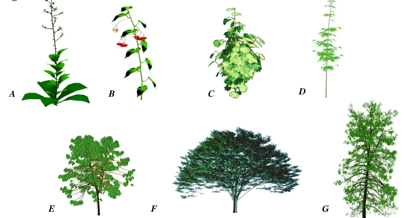
botanical automaton, geometric functions defining organ dimensions and the angles of phyllotaxis, branching and bending of the axes, enable simulations of plant architecture. The result may remains purely geometric (photosynthesis is ignored), but such models can be used in computer graphics to simulate landscapes, or in agronomy to calculate, for example, the interception of light. Such stochastic approach was first applied with the AMAP model (De Reffye et al., 1988, Jaeger and de Reffye, 1992), and applied to numerous species (Figure 4) from which GreenLab’s geometric instantiation and representation of structure are inherited.
Biomass production and partitioning
Ecophysiological variables Ecophysiology considers, on the one hand, the sugars produced by the
leaves (photosynthesis) and used for the functioning of the plant (respiration) and, on the other hand, those used for the production of biomass (cellulose) that gives rise to organ growth. The latter is the carbon fixed on the architecture and is the result of net photosynthesis. Under normal conditions, the proportion of fixed sugars is considered constant.
Accepted Manuscript
12
More or less precise functioning processes may be considered by the model user: for example, organ composition costs or respiration can be taken into account as well (e.g. the cost of sugars is about twice as high for producing oil as for producing cellulose for same weight).
The source-sink concept In our approach, once the functioning of meristems is known, the cohorts of
organs produced with the botanical automaton for each development cycle defines the number of differentiated organ clusters. Some, such as leaves, are source organs. All organs, including leaves, are attractive sinks for the biomass produced. The growth process is also discretized in CD in order to synchronize with development. The growth loop is initiated by the reserves from the seed (Ma et al., 2006).
GreenLab, like several crop models, uses the notion of a common pool that stores synthesized biomass and distributes it to organ compartments. This notion is relevant for herbaceous plants, but lessrealistic for woody trees, ahtough it can be adapted, for instance concerning girth growth (see below).
Source organs Leaves are the source organs of the plant. Crop models consider that dry matter
production is proportional to the intercepted light. The proportionality factor is called "light use efficiency" (LUE). Under standard conditions it can be considered as constant. In the field, dry matter production is found to be proportional to plant transpiration, which is the main limiting factor. The proportionality factor then becomes "water use efficiency" (WUE).
Accepted Manuscript
13
Sink organs The biomass attributed to every organ, distributed from the common pool, is set
proportional to its sink strength. Sink strength varies during the duration of organ expansion tx, following a same form of sink function for all organs of the same type o (o = leaf, internode, fruit, etc.) in a cohort. The function expression is empirically determined; it must adjust to the evolution of the numerical values of the sink strength during organ expansion. In GreenLab, the roots are considered as a single organ with a long expansion duration. Secondary growth is deduced from Pressler's law: for each CD, each active leaf produces a ring element (virtual organ) with a constant sink.
The sink strength of an organ of expansion duration txo is modelled by the function:
( ) (
) (2)
Where the parameter is the strength of the organ sink, t is its chronological age, φ is its
physiological age, o characterizes its type (o = a for the leaf, o = i for the internode, o = f for the
fruit). (
) is the variation function of the sink related to its maturation where txo is the domain
of t for the chronological age of the organ expressed in cycles (txo ≥ 1 and 0 ≤ t ≤ txo).
The GreenLab model defines the sink function according to a discretized beta law function:
( ) ( ) ( ) (3)
where parameters a and b, verifying the constraint a ≥ 1 and b ≥ 1, drive the curve shape; M is a normalization factor.
Plant demand The plant demand D(t) at a given age t is the sum of the active sink organs. Thanks to
the notion of cohorts, the demand can be factorized. The number of phytomers produced by the botanical automaton gives the number of leaves, internodes and fruits produced in each cycle. In the
Accepted Manuscript
14
following equation (eq. 4), organs of type o, physiological age φ and aged u cycles have a sink
function ( ) defined from equation (eq. 2). They appeared in cycle t - u + 1 and are in number
( ). Demand expression D(t) is obtained by a convolution as follows:
( ) ∑ (∑ ( ) ( )) (4)
Calculation of biomass production by the plant Starting from the seed, the calculation of biomass
production and biomass partitioning requires the biomass supply Q in cycle t-1 and demand D in cycle t.
Most crop models use Beer Lambert's law to calculate biomass production per unit of cultivated area and per unit of time :
( ( )) (5)
where Λ is the light use efficiency, I the radiant energy received per surface unit , Sc the cultivated area. LAI is the “leaf area index" (ratio of the leaf area to the cultivated area Sc) and k a coefficient that depends on the average inclination of the leaves. LAI can be measured in the field by an instrument, for instance the Plant Canopy Analyzer (PCA) LAI-2000 (LI-Cor Inc., Lincoln, Nebraska, USA), and the expression ( ( )) estimates the rate of leaf overlapping intercepting light.
The GreenLab model adapts equation (5), which is transformed into:
( ) ( ( ( )
)) (6)
In this expression Q(t) is the amount of biomass synthesized by the plant in cycle t, and Sf(t) is the total plant leaf surface area. The variable Sp is called ‘production surface area’ of the plant and
Accepted Manuscript
15
should be interpreted as an empirical parameter, adjusted to relate the the measured weight of the
plant ( ) ∑ ( ) and its leaf surface area Sf(t).
Computation of organ biomass increment Plant demand D(t) is calculated in each development cycle t using formula (eq. 4). Similarly, the biomass supply Q(t) is calculated by recurrence using formula
(eq. 6).
The biomass growth of an o-type organ depends on the value of its sink and the ratio of the ratio supply synthesized to the previous cycle Q(t - 1) by the current demand D(t). The expansion of the organ of type o appearing in cycle u when the plant is at cycle t (t > u) is written:
( ) ( ) ( )
( ) (7)
The weight of the organ (sum of expansions) that appeared in cycle iu when the plant was at cycle t is then:
( ) ∑ ( ) ( )
( )
(8)
Note that organ o with physiological age φ and appearing at cycle t - u + 1 is represented (
) times as a cohort in the plant structure.
The series ( ) ( ) defines the organic series describing the organ o biomass
profile alonga leafy axis according to the rank of its phytomer.
Allometric relationships define the geometric shape of an organ according to its volume v, which depends on its weight q and density δ, according to the expression: v = q / δ.. The total functional leaf area can then be calculated as:
( ) ∑ ∑ ( ) ( ) ( ) ( ) (9)
Accepted Manuscript
16
Where ta is the duration of leaf functional activity, assumed here to be equal to its expansion duration tx. The index φ denotes physiological age (from 1 to mxφ), da the leaf mass density and ε leaf thickness (assumed constant here). Within a cohort of leaves appearing at chronological age u,
the number of leaves ( ) is recorded, with their individual biomass ( ).
Equation of plant growth recurrence Lastly, by expressing the leaf surface areas as a function of the
previous Q / D ratios, we get the generic recurrence equation that characterizes the individual growth of a computational plant according to the GreenLab model:
( ) ( ( ∑ ∑ ( ) ∑ ( ) ( ) ( ) ( ) ( ) )) (10)
The plant can therefore be broken down as individual parts into a small number of categories of axes, which in turn are broken down into organic series, the description of which gathers all the necessary information contained in development and growth. Through adapted sampling among the organic series, it is possible to define very effective targets for calibration of the sink-source model based on the experimental data. Organic series are built by sampling within the plant architecture. Measurements can be taken over several growth stages (Figure 5).
Application of plant architecture to agronomy: two case studies
Calibration and evaluation of the GreenLab model Evaluation of the model is here based on its
ability to correctly fit organic series, by finding the optimum values of the sink-source parameters using an inverse method. Organic series are outputs of the model and contain the history of growth. The non-linear least squares method is used for this purpose (Guo et al., 2006). Other heuristic methods have also been used, such as particle swarm optimization (Qi et al., 2010), and neural networks (Fan et al., 2015).
Accepted Manuscript
17
We illustrate here the parameter estimations on maize and coffee. Data and sources codes are available as Supplementary Data S1. These are also available from the following link
http://greenlab.cirad.fr/StemGL/AoB_19945R_Codes.zip .
These case studies are somewhat iconic. The study of maize is interesting as it has a simple non-branched deterministic structure but complex organ expansions, due to their duration and sink strength variation. The fruits are not numerous, but their biomass is significant due to their high sink strength. Thus, this example applies to numerous crop plants, such as rice, wheat, tomato, sunflower, etc. Conversely, the coffee tree is a stochastic branched structure. Despite its relative simple structure with only two physiological ages, the establishment of the structure displays a different speed of axis development (the rhythm ratio between trunk and branches is close to ¾), stochastic development both on the trunk and branches, and stochastic ramification with a coupling effect. However, organ expansions are almost immediate and the fruit sink strength is comparable to that of other organs. This example applies for other branched crops, such as cotton, and also for trees in general. Applications of the GreenLab model were also successfully used on temperate and tropical rhythmic species: pine (Wang et al., 2010), maple (Taugourdeau et al., 2019), and teak (Tondjo et al., 2018).
Study of a deterministic example: the case of maize A maize experiment was carried out in France
(Feng et al., 2014). The planting density was d = 7.5 plt/m2, corresponding to the available average
surface area per plant Sd = 1333 cm2/plt. The thermal time-development cycle relationship was
established. Maize stops developing above 21 phytomers, but growth continues. The weights of organ compartments and organic series were measured on plants over 5 growth stages (CD: 10, 14, 19, 27, and 31). For the compartments, each mean and variance on a date corresponded to a sample of 5 plants. For organic series, the average per organ and per rank in the series was taken into account. There were 249 items (organs and compartments) to be adjusted together by the model,
Accepted Manuscript
18
and 13 source-sink parameters to be estimated using the inverse method. The expansion time tx of leaf, sheath and internode increased from the base of the stem and stabilized at the tenth phytomer. This variation could be measured or estimated by optimizing the fit of the organic series. Organ expansion durations usually vary significantly from each other (Figure 6A). The expansion time of the cob was estimated at 30 CDs and that of the tassel at 2 CDs. The leaf thickness parameter was measured as ε = 0.024.
The parameters to be estimated by the inverse method were:
Q0: reserve provided by the seed. Λ: LUE parameter, Sp: plant production area. sSp: standard
deviation of the production area, Pa, Baa : parameters of the blade sink function (Pa = 1); Pp, Bap:
parameters of the sheath sink function. Pi, Bai: parameters of the internode sink function. Pf, Baf:
parameters of the cob sink function. Pm: parameters of the tassel sink function. Secondary sink shape
parameters Bbb, Bbp, Bbf, and tassel sink shape parameters Bam and Bbm were experimentally
defined since Bab, Bap, Baf, asses the shape of the curves for blade, petiole and fruit, while the short
expansion time minimizes the shape effect on the tassel.
The numerical results are presented in Table 2 and in Figure 6C, 6D and 6E. The calculated parameters ensured a good fit of the compartments and organic series at the 5 growth stages (Figure 6D and 6E), meaning that they could be considered as invariant during maize growth.
The method calculated the seed reserve Q0, and a good approximation of Sd =1333 plt/m2, with Sp =1200 plt/m2, which validated the model. The estimated standard deviation of the production area sSp made it possible to correctly estimate the evolution of the standard deviation of
the compartments. The sink of the cob was very high (Pf =2400): the cob captured almost all of the
synthesized biomass during its growth. The variation of the sink strengths are shown in figure 6B.
Accepted Manuscript
19
Using Table 2 providing the parameters used to simulate plant growth, and adding the positions, orientations and the organ shapes, completed the set of parameters necessary to build the plant 3D structure.
Study of a stochastic example: the case of Coffea A Coffea pseudozanguebarie growth study was
undertaken in Ivory Coast with fourteen two-year-old trees. At this stage, no mortality or flowering was observed. We noted the stochastic aspect of the branch sizes from the development, as well as the gradual implementation of branching from the base of the trunk. The absence or presence of branches on the trunk, and their positions, were noted; the organic series measured on trunks and branches from the top were recorded, and the organs were weighed in terms of dry matter.
Results of the organic series analysis The analysis of the organic series then retrieved the source-sink
parameters of coffee tree growth. This stochastic case required transformation of the data using the negative binomial law (Kang et al., 2018). The organic series fitting the results (Figure 7) showed that the GreenLab model was correctly calibrated on this plant. The bottom row of Figure 8 illustrates four 3D simulations using the estimated parameters with additional geometrical parameters (branching angles and phyllotaxy).
Results of the crown analysis The top row of Figure 8 illustrates four observations of crowns in the
study. The crown analysis method (Kang et al., 2018) was used to calculate the development parameters of the trunk (b1 = 0.8) the branches (b2 = 0.9), and the rhythm ratio (w = 0.75).
Accepted Manuscript
20
Comments on the model principles and its emergent behaviour
The concept of the production surface area introduced in equation (eq. 6) is designed to enable the GreenLab model to build the link between the plant on an individual scale (i.e. without light competition) and the stand level. Analysing model behaviour (eq. 6) helps in understanding this concept. At the beginning of growth the Leaf surface area per Production surface area ( the ratio Sf /
Sp ) is small. The expression (eq. 6) then becomes:
( ) ( ) (11)
Growth is proportional to the leaf surface area, meaning that all the leaves separately intercept light: this is then called "free" growth. At this stage, growth is exponential.
After some time, in the case of a high planting density, the foliage covers the entire ground and the ratio k · Sf / Sp is higher. The expression (eq. 6) then becomes:
( ) (12).
Once the competition effect between plants is reached, growth is said to be "limited", becomes constant and proportional to the surface area available on the ground for the plant in competition with its neighbours. Biomass production evolves according to a sigmoid form. Once the effect of competition is reached, Sp must logically approach the available average surface area per plant Sd, according to the planting density: Sd = Sc / d, where Sc is the cultivated area and d is the planting density. So the relationship Sp ≈ Sd should be observed. The validity of Sp = Sd equality in the case of high planting densities has been confirmed on several species for different densities: on maize (Ma et al., 2007), on beetroot (Lemaire et al., 2009), and on tomato (Zhang et al., 2009).
Accepted Manuscript
21
DISCUSSION
Compared with FSPM and crop models, GreenLab’s positioning falls somewhat “in-between”. What are the benefits of this approach for agronomy, seen as a voluntarily simplified model from an ecophysiological point of view and from a structural (geometrical) point of view?
Validation of the GreenLab model on crop plants and its positioning.
The GreenLab approach shows genericity of the model when applied to crop plants, even when faced with various plant architectures. In our studies, architectural variability was wide, covering continuous growth to rhythmic growth, on both temperate and tropical species, potentially modelling the stochastic effects of phytomer development, branching and viability. Indeed, for about twenty crop plants (grasses, shrubs and trees) parameters were satisfactorily estimated for the GreenLab model (Figure 9). The development and growth parameters, using the crown and organic series analysis, were computed successfully and fitted the data well. They validated the model application and illustrated its genericity. Moreover, on these plants, the set of estimated parameters showed good stability under various climatic conditions, and most could be considered as invariant (Ma et al., 2007 and Kang et al., 2012). Thus, GreenLab position itself as a generic model that capture the key development and functional feature of plants with minimal equations.
The GreenLab model is a "source-sink solver", i.e. a tool for finding the source-sink dynamics of a plant during its past growth. A very important point when using models in agronomy is the measurement sampling strategy. The GreenLab model uses the different axis types (physiological ages) and their grouping into crowns and organic series. These entities, which are generic and adapted to all architectural models, support the calibration of the model, using efficient inverse methods for parameter estimation. Moreover, missing data due to organ abortion are no longer a drawback. From a correctly collected sample, we can reconstruct the history of demand and biomass supply for each development cycle, using crown and organic series analyses.
Accepted Manuscript
22
In plant breeding, the growth parameters of the GreenLab model can be considered, as a first approximation, as invariant, because the source-sink relationships are relatively independent of the environmental parameters. The establishment of relationships between these parameters and QTLs should lead to effective selection in the search for ideotypes (Letort et al., 2008).
In the context of phenotyping, where FSPM models are beginning to be used (Luquet et al., 2012), the Greenlab model provides an effective framework for streamlining trait measurements and their analysis according to organic series.
Switch from individual plant to stand
Introducing the notion of plant architecture in agronomy in its botanical component is relevant from an ecological point of view (De Reffye et al., 2009); compared to crop models that generally consider a stand scale, Greenlab seeks a better representation of plant growth and stand production by using the concept of plant architecture as a support for plant functioning. Greenlab’s approach has relatively few parameters (usually a few dozen to simultaneously fit individual organ mass at several stages of plant growth), compared to most other FSPMs. Biomass computation from the production surface area and functioning leaf area is efficient (Beer Lambert’s Law and not computation of explicit light interception with organ geometries) as shown in the comparison with photon ray tracing used by (Wang et al., 2012). GreenLab model and its approach at plant level is fully ecophysiogically compatible with crop models that use only compartments. Crop models can be considered as a projection of the GreenLab model, which uses either phytomers, or compartments. Thus, the GreenLab model enables a switch from the functioning of the individual plant to that of the stand, with the use of production area parameter Sp, related to planting density. As shown by (Baey et al., 2014), compared to crop models such as Stics, Ceres, Pilot, etc., GreenLab shows a comparable performance working in compartment mode. Taking into account planting density, germination times and the calculated variance of Sp makes the calculated LAI and production similar to those calculated by a crop model (Feng et al., 2014).
Accepted Manuscript
23
CONCLUSION
GreenLab’s approach reflects a macroscopic approach, relating to the phytomer level. It does not provide an understanding of fine physiological processes. However, the approach is of particular interest in terms of genericity, complexity and computational performance, and its ability to estimate source-sink relations. Its formalism also allows the switch from the individual plant scale to the crop/stand level.
GreenLab’s approach has helped to take up the challenge of reproducing the growth dynamics of all organs with a very limited set of parameters. Development of the GreenLab model has always paid careful attention to the parameter estimation methodology. The organic series, i.e. the sequence of organs along the axis, defines the core key for defining relevant measurement strategies and experimental protocols allowing a wide range of applications.
This approach retains a degree of rigidity; it assumes that the development of the potential structure follows invariant kinetics according to thermal time. In other words, feedback (other than external interactions) between growth and development is ignored. However, promising studies has been undertaken to overcome these difficulties. The kinetic approach dependency to the thermal time of the sinks can be replaced by the supply to demand ratio (Q / D), giving equivalent adjustments (Zhang et al., 2009). Similarly, the numerical values of development, mortality and branching rates found by the crown method can be linked to functions depending on Q / D (De Reffye et al., 2018). Thus, we are currently upgrading the model with the feedback effect of the internal trophic competition, represented by the ratio of biomass supply to demand, contributing to a new way to plant structural plasticity understanding.
Accepted Manuscript
24
LITERATURE CITED
Allen M.-T., Prusinkiewicz P., and DeJong T.-M., 2005. Using L-systems for modeling
source-sink interactions, architecture and physiology of growing trees: the L-PEACH model.
New Phytologist, 166 (3): 869-880.
Baey C., Didier A., Lemaire S., Maupas F., and Cournède P.-H., 2014. Parametrization of five
classical plant growth models applied to sugar beet and comparison of their predictive capacities on root yield and total biomass. Ecological Modelling, 290: 1120.
Barthélémy D, and Caraglio Y., 2007. Plant architecture: a dynamic, multilevel and comprehensive
approach to plant form, structure and ontogeny. Annals of Botany 99: 375–407.
Boudon F., Pradal C., Cokelaer T., Prusinkiewicz P., and Godin C., 2012. L-Py: an L-system simulation
framework for modeling plant architecture development based on a dynamic language. Frontiers in
plant science, 3, 76.Brisson N., Mary B., Ripoche D., Jeuffroy M. H., Ruget F., Nicoullaud B., Richard G., Beaudoin N, Recous S, Tayot X, Plénet D, Cellier P, Machet J.-M., Meynard J.-M., and Delécolle R., 1998. STICS: a generic model for the simulation of crops and their water and nitrogen balances. I.
Theory and parameterization applied to wheat and corn. Agronomie, 18(5-6): 311-346.
Buis R., and Barthou H., 1984. Relations dimensionnelles dans une série organique en croissance
chez une plante supérieure. Rev. Biomath., 85: 1-19.
Casadebaig P., Guilioni L., Lecoeur J., Christophe A., Champolivier L., and Debaeke P., 2011.
SUNFLO, a model to simulate genotype-specific performance of the sunflower crop in contrasting environments. Agricultural and forest meteorology, 151(2): 163-178.
Cieslak M., Seleznyova A.-N., and Hanan J., 2011. A functional–structural kiwifruit vine model
integrating architecture, carbon dynamics and effects of the environment. Annals of Botany, 107 : 747–764. doi: 10.1093/aob/mcq180
Dabadie P., De Reffye P., and Dinouard P., 1991. Modelling bamboo growth and
architecture: Phyllostachys viridi-glaucescens Rivière A. et C. Journal of the American Bamboo
Society, 8 (1-2): 65-79.
De Reffye P., 1981 a. Modèle mathématique aléatoire et simulation de la croissance et de
l'architecture du caféier Robusta. I. Etude du fonctionnement des méristèmes et de la
croissance des axes végétatifs. Café Cacao Thé, 25 (2): 83-104
Accepted Manuscript
25
De Reffye P., 1981 b. Modèle mathématique aléatoire et simulation de la croissance et de
l'architecture du caféier Robusta. II. Etude de la mortalité des méristèmes plagiotropes. Café
Cacao Thé, 25 (4) : 219-229
De Reffye P., 1982. Modèle mathématique aléatoire et simulation de la croissance et de
l'architecture du caféier Robusta. III. Etude de la ramification sylleptique des rameaux
primaires et de la ramification proleptique des rameaux secondaires. Café Cacao Thé, 26 (2):
77-96.
De Reffye P., Edelin C., Françon J., Jaeger M., and Puech C., 1988. Plants models faithful to botanical
structure and development. Computer Graphics, 22 (4): 151-158. Siggraph'88, 1988-08-01/1988-08-05, Atlanta, Etats-Unis.
De Reffye P., Cognée M., Jaeger M., and Traoré B., 1988. Modélisation stochastique de la
croissance et de l'architecture du cotonnier. 1. Tiges principales et branches fructifères
primaires, Coton et Fibres Tropicales, 43 (4): 269-291.
De Reffye P., Dinouard P., and Barthélémy D., 1991. Modélisation et simulation de l’architecture de
l’Orme du Japon Zelkova serrata (Thunb.) Makino (Ulmaceae) : la notion d’axe de référence.
Comptes Rendus du 2e Colloque international sur l’arbre, Montpellier, 10-15 Septembre 1990.
Naturalia Monspeliensia, Hors-Série : 251-266.
De Reffye P., Elguero E., and Costes E., 1991. Growth units construction in trees: a
stochastic approach. Acta biotheoretica (39): 325-342.
De Reffye, P., Heuvelink, E., Guo, Y., Hu, B.-G., and Zhang, B.-G., 2009. Coupling process-based
models and plant architectural models: a key issue for simulating crop production. In Crop modeling
and decision support (pp. 130-147). Springer, Berlin, Heidelberg.
De Reffye, P., Jaeger, M., Barthélémy, D., and Houiller, F., 2016. Architecture et croissance des plantes: Modélisation et applications. Editions Quae, 2016, Synthèses, 978-27592-2622-1
De Reffye P., Jaeger M., Sabatier S., and Letort V., 2018. Modelling the interaction between
functioning and organogenesis in a stochastic plant growth model: Methodology for parameter estimation and illustration. In 2018 6th International Symposium on Plant Growth Modeling,
Simulation, Visualization and Applications (PMA), IEEE., 102-110
De Reffye P., Jaeger M., Barthélémy D., and Houllier F., 2018. Architecture des plantes et production végétale. Éditions Quæ
Diao J., De Reffye P., Lei X., Guo H., and Letort V., 2012. Simulation of the topological development
of young eucalyptus using a stochastic model and sampling measurement strategy. Computers and
electronics in agriculture, 80 (1): 105-114.
[20120113]. http://dx.doi.org/10.1016/j.compag.2011.10.019
Eschenbach C., 2005. Emergent properties modelled with the functional structural tree growth
model ALMIS: computer experiments on resource gain and use. Ecological Modelling, 186: 470–488
Accepted Manuscript
26
Fan X.-R., Kang M.-Z., Heuvelink E., De Reffye P., and Hu B.-G., 2015. A knowledge-and-data-driven
modeling approach for simulating plant growth: A case study on tomato growth. Ecological
Modelling, 312: 363-373
Feng L., Mailhol J.-C., Rey H., Griffon S., Auclair D., and De Reffye P., 2014. Comparing an empirical
crop model with a functional structural plant model to account for individual variability. European
Journal of Agronomy, 53: 16-27.
Griffon S., and De Coligny F., 2014. AMAPstudio: an editing and simulation software suite
for plants architecture modelling. Ecological Modelling, 290: 3-10
Guédon Y., Caraglio Y., Heuret P., Lebarbier E., and Meredieu C., 2007. Analyzing
growth components in trees. Journal of Theoretical Biology, 248 (3): 418-447.
Guo Y., Ma Y., Zhan Z., Li B., Dingkuhn M., Luquet D., and De Reffye P., 2006. Parameter
optimization and field validation of the functional-structural model GREENLAB for maize. Annals of
Botany, 97 (2): 217-230.
Guo Y., Fourcaud T., Jaeger M., Zhang X.-P., and Li, B.-G., 2011. Plant growth and
architectural modelling and its applications. Annals of Botany, 107(5): 723-727.
Hallé F., Oldeman R.-A.-A., and Tomlinson P.-B., 1978. Tropical Trees and Forests.
Springer Verlag, Berlin, Heidelberg, New-York, 441p.
Heuvelink E. 1998. Evaluation of a dynamic simulation model for tomato crop growth and
development. Annals of Botany 83: 413-422.
Henke M., Kurth W., and Buck-Sorlin G.-H., 2016. FSPM-P: towards a general functional-structural
plant model for robust and comprehensive model development. Frontiers of Computer Science, 10(6): 1103-1117
Hua J., Kang M.-G., and de Reffye P., 2011. An Interactive plant pruning system based on GreenLab
model: Implementation and case study. In 2011 IEEE International Conference on Computer Science
and Automation Engineering, IEEE, 4, 185-188
Jaeger M. and De Reffye P., 1992. Basic concepts of computer simulation of plant growth. Journal of biosciences, 17 (3): 275-291.
Jaeger M., De Reffye P., Sabatier S., Letort V., Heuvelink E., Caraglio Y., Motisi N., Kang M.-G., and Zhang B.-G., 2015. Plant growth architecture and production dynamics (UVED online course
modules). http://greenlab.cirad.fr/GL_UVED/ . Last successful access: 2019/11/04
Kang M.-G., Wang X.-W, Qi R., and De Reffye, P., 2009. GreenScilab-Crop, an open source software
for plant simulation and parameter estimation. In : 2009 IEEE International Workshop on
Open-source Software for Scientific Computation (OSSC). IEEE, 2009. 91-95
Kang M.-Z, Heuvelink E., Carvalho S.-M., and De Reffye P., 2012. A virtual plant that responds to the
environment like a real one: the case for chrysanthemum. New Phytologist, 195(2): 384-395.
Accepted Manuscript
27
Kang M.-Z., Hua J., Wang X., De Reffye P., Jaeger M., and Akaffou S., 2018. Estimating Sink
Parameters of Stochastic Functional-Structural Plant Models Using Organic Series-Continuous and Rhythmic Development. Frontiers in Plant Science, 9, 1688
Keating B.-A., Carberry P.-S., Hammer G.-L., Probert M.-E., Robertson M.-J.,
Holzworth D., and McLean G., 2003. An overview of APSIM, a model designed for
farming systems simulation. European Journal of Agronomy, 18(3): 267-288.
Kniemeyer O., 2004. Rule-based modelling with the XL/GroIMP software. The logic of artificial life. Proceedings of 6th GWAL. AKA Akademische Verlagsges Berlin, 56-65
Lecoustre R., De Reffye P., Jaeger M., and Dinouard P., 1992. Controlling the Architectural
Geometry of a Plant’s Growth—Application to the Begonia Genus. In: Creating and animating the
virtual world. Springer, Tokyo, 1992. p. 199-214.
Lemaire S., Maupas F., Cournède P.-H., Allirand J.-M., De Reffye P., and Ney B., 2009. Analysis of
the density effects on the source-sink dynamics in sugar-beet growth. In 2009 Third International
Symposium on Plant Growth Modeling, Simulation, Visualization and Applications (PMA09), IEEE,
285-292
Letort V., Mahe P., Cournède P.-H., de Reffye P., and Courtois B., 2008. Quantitative genetics and
functional-structural plant growth models: Simulation of quantitative trait loci detection for model parameters and application to potential yield optimization. Annals of Botany, 101(8): 1243-1254.
Luquet, D., Dingkuhn, M., Kim, H., Tambour, L., and Clement-Vidal, A., 2006. EcoMeristem, a model
of morphogenesis and competition among sinks in rice. 1. Concept, validation and sensitivity analysis. Functional Plant Biology, 33(4): 309-323.
Luquet, D., Rebolledo, M. C., and Soulie, J. C., 2012. Functional-structural plant modeling to support
complex trait phenotyping: case of rice early vigour and drought tolerance using ecomeristem model. In 2012 IEEE 4th International Symposium on Plant Growth Modeling, Simulation,
Visualization and Applications, IEEE, 270-277.
Ma Y.-T. Guo Y. Zhan Z.-G. Li B.-G., and De Reffye P., 2006. Evaluation of the Plant Growth Model
GREENLAB-Maize. Acta Agronomica Sinica, Science Press, Chinese Academy of Sciences, 32 (7): 956-963
Ma Y.-T., Li B.-G., Zhan Z.-G., Guo Y., Luquet D., De Reffye P., Dingkuhn M., 2007. Parameter
stability of the functional–structural plant model GREENLAB as affected by variation within populations, among seasons and among growth stages. Annals of Botany, 99(1): 61-73.
Mailhol J.-C., Ruelle P., Walser S., Schütze N., and Dejean C., 2011. Analysis of AET and yield
prediction under surface and buried drip irrigation systems using the crop model PILOTE and Hydrus-2D. Agric. Water Manag., 98: 1033-1044.
Mathieu A., Letort V., Cournède P.-H., Zhang B.-G., Heuret P., and De Reffye P., 2012.
Oscillations in Functional Structural Plant Growth Models Math. Model. Nat. Phenom. 7(6):
47–66.
Accepted Manuscript
28
Perttunen J., Sievänen R., and Nikinmaa E., 1998. LIGNUM: a model combining the
structure and the functioning of trees. Ecological Modelling, 108(1-3): 189-198.
Poisson C., Rey H., 1997. « Modélisation de l’architecture et de la croissance de 5 espèces du genre Nicotiana. » Ann. Du Tabac, Section 2, 29: 37-54.
Pressler R., 1865. Das Gesetz der Stammbildung. Arnoldische Buchhandlung (Leipzig),
153 p.
Prusinkiewicz P., Lindenmayer A., and Hanan J., 1988. Developmental models of herbaceous plants
for computer imagery purposes, Proceedings of the 15th annual conference on Computer graphics, p.141-150, August 01-05, 1988, Atlanta, Georgia, United States.
Qi R., Ma Y.-T., Hu B.-G., De Reffye P., and Cournède P.-H., 2010. Optimization of source–sink
dynamics in plant growth for ideotype breeding: A case study on maize. Computers and Electronics in
Agriculture, 71(1) : 96-105.
Ribeyre F., Jaeger M., Ribeyre A., and De Reffye P., 2018. StemGL, a FSPM tool dedicated to crop plants model calibration in the single stem case. In Proceedings of 6th International Symposium on Plant Growth Modeling, Simulation, Visualization and Applications (PMA2018), IEEE, 33-38
Rivals P., 1965. Essai sur la croissance des arbres et sur leurs systèmes de floraison (Application aux
espèces fruitières). Journal d’Agronomie Tropicale et de Botanique Appliquée, 12: 655-686.
Sievänen R., Godin C., DeJong T.-M., and Nikinmaa E., 2014. Functional–structural plant models: a
growing paradigm for plant studies. Annals of Botany, 114(4): 599-603
Smoleňová K., Henke M., and Kurth W., 2012. Rule-based integration of GreenLab into GroIMP with
GUI aided parameter input. In 2012 IEEE 4th International Symposium on Plant Growth Modeling,
Simulation, Visualization and Applications, IEEE, 347-354
Taugourdeau O., Delagrange S., Lecigne B., Sousa-Silva R., and Messier C., 2019. Sugar maple (Acer
saccharum Marsh.) shoot architecture reveals coordinated ontogenetic changes between shoot specialization and branching pattern. Trees, 1-11.
Tondjo K., Brancheriau L., Sabatier S., Kokutse A.-D., Kokou K., Jaeger M., De Reffye P., and Fourcaud T., 2018. Stochastic modelling of tree architecture and biomass allocation: application to
teak (Tectona grandis L. f.), a tree species with polycyclic growth and leaf neoformation. Annals of
botany. 121(7): 1397-1410.
Viennot X., Eyrolles G., Janey N., Arqués D., 1989, Combinatorial analysis of ramified patterns and
computer imagery of trees, ACM SIGGRAPH Computer Graphics, 23(3): 31-40
Wang F., Kang M.-G., Lu Q., Letort V., Han H., Guo Y., De Reffye P., and Li B.-G.,
2010. A stochastic model of tree architecture and biomass partitioning: application to
Mongolian Scots pines. Annals of Botany. 107(5): 781-792.
Wang H., Kang M.-G., and Hua J. 2012. Simulating plant plasticity under light
environment: A source-sink approach. In 2012 IEEE 4th International Symposium on Plant
Growth Modeling, Simulation, Visualization and Applications, IEEE, 431-438.
Accepted Manuscript
29
Wang H.-Y., Kang M.-Z., Hua J., and Wang X.-J., 2013. Modeling plant plasticity from
a biophysical model: Biomechanics. In Proceedings of the 12th ACM SIGGRAPH
International Conference on Virtual-Reality Continuum and Its Applications in Industry,
ACM, 115-122
Wernecke P., Buck-Sorlin G. and Diepenbrock W., 2000. Combining process- with
architectural models: the simulation tool VICA. Systems Analysis Modelling Simulation, 39
(2): 235-277.
Yan H.-P., De Reffye P., Pan C.-H, and Hu B.-G., 2003. Fast construction of plant architectural models
based on substructure decomposition. Journal of Computer Science and Technology, 18(6): 780-787.
Zhang B.-G, Kang M.-Z, Letort V., Wang X.-X., and De Reffye P., 2009, Tomato plant. In 2009 Third International Symposium on Plant Growth Modeling, Simulation, Visualization and Applications. IEEE Proccedings of PMA09, 191-197
Zhao X., De Reffye P., Barthélémy D., and Hu B.-G., 2003. Interactive simulation of plant
architecture based on a dual-scale automaton model. In Hu B., Jaeger M. (Eds), Plant growth
modelling and applications (PMA03), Proceedings of the 2003' International Symposium on Plant Growth Modeling, Simulation, Visualization and Their Applications, Beijing, Chine, 13-16 oct. 2003.
Beijing: Tsinghua University Press, Springer; 144-153.
Yan H.-P., Kang M.-Z., De Reffye P, and Dingkuhn M. 2004. A dynamic, architectural plant model
simulating resource-dependent growth. Annals of Botany 93: 591-602.
Accepted Manuscript
30
TABLES
Table 1. Terms of GreenLab model entities, parameters and variables, alphabetically sorted. CD, GU and o are entity definitions standing respectively for the cycle of development defined by thermal time, the growth unit, expressed as a successive list of CDs, and for organ generic notation (o is to be replaced in context with leaf, petiole, internode, etc.). The variable t stands for the current CD. All variables are normalized to one CD so the time unit “per CD” is omitted, for the sake of clarity.
Concerning plant development, the number of physiological ages is maxφ, standing for the number of different axis typologies in the modelled plant; a, b, c and w define the development parameters, respectively standing for the branching, development, viability and rhythm ratio rates. They are defined from statistics based on plant axis phytomer distributions. From these, development
simulation defines the organ cohorts Nφo(u), i.e. the number of organs o of age u and physiological
age φ, in each growth cycle t (i.e. appearing in cycle t-u).
Concerning now production, the model parameters to be fitted using a target file filled with sparse
organ weight measurements are those related to organ o sink strengths, Po, Bao and Bbo respectively
standing for the sink strength value (Po) and its variation during organ expansion (Bao and Bbo define
the variation shape) and those related to biomass production at plant level, Q0, the seed biomass,
Sp, the production surface area and Λ, light use efficiency. These parameters define plant demand D(t) and production Q(t) in each cycle t, computing the functional leaf area Sf(t) from the various
leaf cohorts and leaf thickness ε.
Accepted Manuscript
31
Bao No unit Organ o sink strength variation Beta law first parameter
Bbo No unit Organ o sink strength variation Beta law second parameter
CD No unit Cycle of development
GU CD Growth Unit
a No unit Branching rate (probability), aφ is indexed to physiological age φ
b No unit Development rate (probability), possibly indexed to physiological age φ
c No unit Viability, possibly indexed to physiological age φ
D(t) No unit Plant demand at cycle t
I MJ.cm−2 Radiant energy received per surface unit during one cycle
Nφo(u) No unit Number of organs o of physiological age φ of u cycles
maxφ No unit Maximum physiological age
o No unit Generic organ (o = a: leaf; o = i: internode; o = p: petiole; o = f:
female fruit; o = m: male fruit)
Po No unit Organ o sink strength function
Q(t) g Biomass produced at plant level during cycle t
Q0 g Seed biomass, stands for Q(0)
qφo(t) g Biomass of one organ o of physiological age φ produced in cycle t
Sf(t) cm2 Leaf area functioning in cycle t
Sp cm2 Plant production surface area
Accepted Manuscript
32
Sd cm2 Available surface area per plant (= cultivated area / number of plants)
t CD Current cycle of development, depending on thermal time
TQ(t) g Total biomass produced at plant level from cycles 1 to t
w No unit Rhythm ratio
ε cm Leaf thickness
φ No unit Current physiological age
Λ g·MJ-1 Light use efficiency
Accepted Manuscript
33
Table 2. Model parameter values. Parameters Bba to Bbm relative to organ sink strength variation
were empirically estimated; parameters Q0 to Pm were then calculated by the least squares method.
Λ: Light use efficiency, Sp: Production surface area, sSp: Sp variation, Pa: Leaf sink strength, Baa: Leaf
sink strength variation parameter 1, Pp: Petiole sink strength, Bap: Petiole sink strength variation
parameter 1, Pi: Internode sink strength, Bai: Internode sink strength variation parameter 1, Pf: Cob
sink strength, Baf: Cob sink strength variation parameter 1, Pm: Tassel sink strength, Bba: Leaf sink
strength variation parameter 2, Bbp: Petiole sink strength variation parameter 1, Bbf: Cob sink
strength variation parameter 2, Bam: Tassel sink strength variation parameter 1, Bbm: Tassel sink
strength variation parameter 2.
Q0 (g) 1.1 Λ (g·MJ-1) 0.056 Sp (cm2) 1200 sSp (cm2) 160 Pa (No unit) 1 Baa (No unit) 2.7 Pp (No unit) 0.91 Bap (No unit) 2.2 Pi (No unit) 2.5 Bai (No unit) 4.1 Pf (No unit) 2400 Baf (No unit) 7.3 Pm (No unit) 4.2