Adaption to a varying auditory environment

Adaptation to a Varying Auditory Environment

by

Gregory Galen Lin

Submitted to the Department of Electrical Engineering and

Computer Science

in partial fulfillment of the requirements for the degree of

Bachelor of Science in Electrical Science and Engineering

and Master of Engineering in Electrical Engineering and Computer

Science

at the

MASSACHUSETTS INSTITUTE OF TECHNOLOGY

May 1996

@

Gregory Galen Lin, MCMXCVI. All rights reserved.

The author hereby grants to MIT permission to reproduce and

distribute publicly paper and electronic copies of this thesis

document in whole or in part, and to grant others the right to do so.

A uthor

...

Department of Elf'ctricdal Engineering and Computer Science

May 28, 1996

Certified by

,Nathaniel I Durlach

Research Scientist

:5hesis Supervisor

Accepted

b-y-

_{Fred&r; R. Morgenthaler}

Chairman, Department Committee on Graduate Students

OF TECHNOLOGY

Adaptation to a Varying Auditory Environment

by

Gregory Galen Lin

Submitted to the Department of Electrical Engineering and Computer Science on May 28, 1996, in partial fulfillment of the

requirements for the degree of

Bachelor of Science in Electrical Science and Engineering

and Master of Engineering in Electrical Engineering and Computer Science

Abstract

This project investigated sensorimotor adaptation to rearranged auditory cues. Data was collected by presenting subjects with an acoustic cue (a gated pulse-train gen-erating a clicking sound) simulated to come from one of 13 locations (confined to a horizontal azimuthal plane) and recording the subject's estimate of the stimuli loca-tion. After each response, the subject was informed of the correct response, providing constant training. Subjects were presented, in order, with unaltered cues, strongly altered cues, weakly altered cues, and unaltered cues. Results show that, in addition to partial adaptation to the changing environment, subjects can partially adapt from strongly altered cues to weakly altered cues.

Thesis Supervisor: Nathaniel I Durlach Title: Senior Research Scientist

Contents

5.6 Imperfection in auditory cues 5.7 Impact of edges ...

6 Summary

A Warp and Line Fit Results

7 7 8 10 10 10 15 16 17 17 18 27 33 33 35 37 . . . . . . . . . . . . ...

List of Figures

2-1 Transformation performed by fn(0) ...

3-1 Altered Locations: (a) normal cues (n = 1); (b)

cues (n = 4); (c) first set of altered cues (n = 2)

5-1 Runs 2 and 3: Changing from n = 1 to n= 4 .

5-2 Runs 3 and 17: Start and finish of n = 4 . . . .

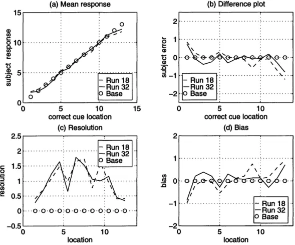
5-3 Runs 17 and 18: Changing from n = 4 to n = 2

5-4 Runs 18 and 32: Start and finish of n = 4 . . .

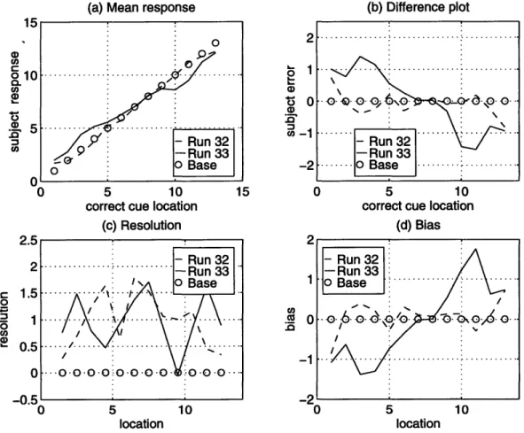
5-5 Runs 32 and 33: Changing from n = 2 to n = 1

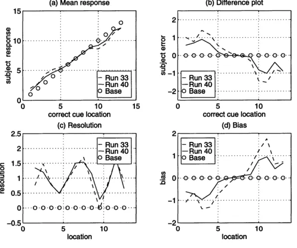
5-6 Runs 33 and 40: Start and finish of n = 1 . . .

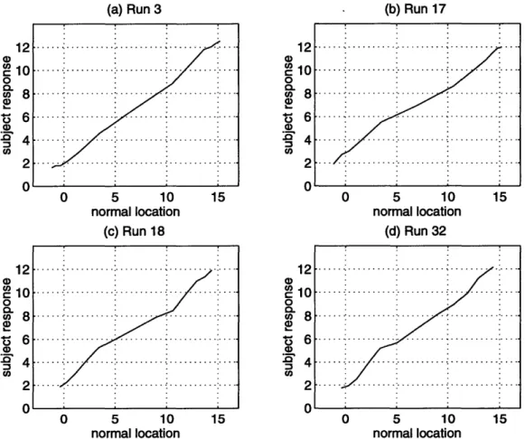
5-7 Observation of linearity ... 5-8 Individual Adaptation Results ... 5-9 Adaptation over runs ...

second set of altered

. . . . . 14 . . . . . 21 . . . . . 22 . . . . . 23 . . . . . 24 . . . . . 25 . . . . . 26 . . . . 28 . . . . 30 . . . . 32

List of Tables

3.1 Table of Warp Transformations ... 12

5.1 Subject Exponential Fit Results ... 30

A.1 Line-Fit values ... ... 38

Chapter 1

Project

This project investigated subject adaptation to supernormal auditory localization cues. Supernormal auditory localization aims to improve a subject's ability to dis-criminate the locations of nearby sounds. The proposed experiments will contribute to the understanding of adaptation to supernormal auditory localization cues.

Chapter 2

Background

2.1

Localization Cues

Sound localization involves processing of three main indicators: interaural intensity difference (IID), interaural time difference (ITD), and spectral cues. IIDs are dif-ferences in sound intensity between the subject's ears, where, for example, a more intense sound at the left ear is more likely to correspond to a source on a person's left. ITDs are any differences in sound arrival times between the ears; the closer an ear is to a sound source, the earlier the ear will receive the sound. As in the case with IIDs, ITDs between the two ears help indicate the location of the sound source. The final main indicator used in auditory localization is monaural spectral cue shaping. The outer ear alters a sound according to the sound's frequency and the angle with which it impacts the ear. Unlike IIDs and ITDs, monaural frequency cues depend on the prior knowledge and experience of the subject with these frequency-to-location translations [2].

Localization cues are generated when a sound interacts with a person's head, and the total interaction can be summarized by a head-related transfer function (HRTF). By measuring the intensity, time, and frequency changes of a known source as it enters the ear canal from different locations, a set of coefficients can be determined such that convolution of these coefficients with an audio stream will produce correct spatial signals for the left and right ear.

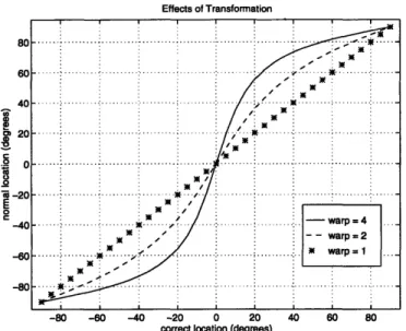
80 60 40 Q 20 0 0 7M -20 -40 -60 -80 Effects of Transformation --... .... .4. - i· i i: i i-· - -- : - M ... ... ... .... - warp = 4 S-- warp = 2 3K Na warp = )- X a .... . .. . . . .a . . . . .*. . . . . . . . . .. . . -80 -60 -40 -20 0 20 40 60 80

correct location (degrees)

Figure 2-1: Transformation performed by f,(O)

2.2

Previous Work

In this project, subjects were exposed to an auditory spatial distortion constrained along a constant azimuthal plane described by the expression:

1 2n sin(20)

0'

=

f,(0)

=

1 tan-[

2n

sin(2

where the angle, 9, represents the correct location, 0' is the angle that normally corresponds to the localization cues presented to the subject, and n represents the extent of the audio warping.

The term correct will always refer to the location from which the subject is told the source is coming, and the term normal will refer to the location that normally corresponds to the physical cues presented. Thus, subjects are told that the source is at 0, even though the normally-heard position of the source is 0'. The degree of distortion produced by n (or warp) is reflected in figure 2-1 where the x-axis reflects the correct location and the y-axis denotes the normal location. As shown in figure

2-1, a value of n = 1 represents no altering, so that the correct cue locations and normal

cue locations are the same. Larger values of n represent more drastic deviations from normal.

When the transformed cues are first introduced, subjects will make systematic

errors in localization. For instance, with n > 1, subjects will tend to hear sounds farther off-center than normal. A subject's adaptation to the transformed audio cues is observed through analysis of their localization performance, summarized by

resolu-tion and bias measures. Adaptaresolu-tion is evidenced if subjects overcome the systematic

error (bias) in localization judgements over time.

Previous work [1] has shown that subjects can partially adapt within a two-hour period (e.g. over time, bias is reduced) when they are exposed to a single cue trans-formation of the form shown in figure 2-1. Subjects also adapted to a relatively weak

transformation (n = 2) followed by a stronger transformation (n = 4) in a single

2-hour session. A single model was able to explain both of these results. However, a pilot study with only 2 subjects indicated that subjects given a relatively strong

transformation (n = 4) followed by a relatively weak transformation (n = 2) did not

adapt in a way predicted by the model. The work described here investigates the surprising result in more detail.

Chapter 3

Data Collection

3.1

Task

Data was collected through a series of trials with each subject. Each trial consisted of a burst of clicks, after which the subject responded with the apparent location of the sound source. The response was immediately followed by visual feedback from spatially-positioned light bulbs (fig. 3-1) giving the correct sound source position. Testing and training were thus simultaneous, with each trial adding to the subject's experience with the new auditory space.

Twenty-six trials were grouped to form a run, with a stretch of 40 runs making up a session (typically spanning two hours). In each session, subjects were exposed to,

in order, 2 runs of normal cues (warp parameter n = 1), 15 runs of strongly warped

cues (n = 4), 15 runs of mildly warped cues (n = 2), and 8 final runs of normal cues

(n = 1) with a 5 minute break after the 10th and 32nd runs. Subjects were notified

each time the degree of warping is changed.

3.2

Setup

Subjects were seated facing 13 numbered lights labeled 1 to 13 from left to right. The lights were arranged on a semi-circular path at 10 degree intervals, 5 feet from the subject. Light 7 was visually straight ahead and referenced as 0 degrees, light 1 was

located at -60 degrees, and light 13 was located at +60 degrees.

With the normal set of cues (fig. 3-1a) each light corresponded to its physical location. Under strongly warped cues (fig. 3-1c), the "normal" sound location corre-sponding to each lamp was shifted farther off center than the actual lamp location. For example, the sound cues for location number 8 were closer to the normal cues for a source at +30 degrees than for the normal cues for a normal source at +10 degrees (under no warping). The lightly warped cues (fig. 3-1b) gave the same type of distortion as the strongly warped cues (fig. 3-1c), but to a lesser extent (table 3.1).

light f (O)n = 1 f (O)n =4 f (O)n = 2 -90.00 -90.00 -90.00 -80 -87.48 -84.96 -70 -84.8 -79.69 1 -60 -81.79 -73.9 2 -50 -78.15 -67.24 3 -40 -73.41 -59.21 4 -30 -66.59 -49.11 5 -20 -55.52 -36.05 6 -10 -35.2 -19.43 7 0 0 0 8 10 35.2 19.43 9 20 55.52 36.05 10 30 66.59 49.11 11 40 73.41 59.21 12 50 78.15 67.24 13 60 81.79 73.9 70 84.8 79.69 80 87.48 84.96 90 90 90

The head position of the subject was monitored using a Bird headtracker (a com-mercial device using electro-magnetic pulses to allow the position of the head to be tracked) mounted on a set of Sennheiser HD-545 headphones. The acoustic stimu-lus was five 1 millisecond pulses spaced at 100 millisecond intervals sent through a low-pass filter (to prevent aliasing of high-frequency components) and into a

Con-volvotron.

The Convolvotron was special-purpose signal-processing hardware installed in an Intel x86-based PC responsible for mapping an input source to the appropriate lo-cation in auditory space. The input signal was first sampled and digitized, then the mapping was accomplished by convolving the input with a pair of transfer functions, one for the right ear and one for the left ear, which contain the direction-dependent effects on sound caused by a head and a pair of ears. This pair of transfer functions was simply the empirically-determined HRTF for a source from the specified direc-tion. Thus, any auditory signal was transformed into a pair of signals (left and right) that contain spatial information.

From the Convolvotron, the newly spatialized signal was sent to the headphones. After each presentation, the subject entered a responses (between 1 and 13, corre-sponding to the numbered sources) on a keyboard which sat on their lap. From the keyboard, the PC collected the response, and after each response, activated the lamp corresponding to the correct sound source position. Through this feedback, the sub-ject was trained to adapt to changes in the mapping between audio cues and the corresponding correct location. Data files with subject responses (recorded by the PC) were updated after every run.

-60 -90 -90 . 6o' '90 -30 -o0 0* -.30

Figure 3-1: Altered Locations: (a) normal cues (n = 1); (b) second set of altered cues

(n = 4); (c) first set of altered cues (n = 2)

14 -10· i :o· 9d .. ,.

0o

Chapter 4

Experimental Problems

The setup had a few shortcomings that may affect the experimental results. Ex-periments prior to January 8th, 1996 were conducted in an office room that is not sound-proof. While the headphones provided some isolation they could not completely eliminate the noises caused by the environment. In addition to the computer's con-tinual mechanical hum, the disk-writing operation that occurred between runs was audible to the subject. Experimentation after January 8th was conducted in a sound-proof room with the PC located outside of the booth. With this setup, the primary disturbance was a noticeable hum produced by the Bird head-tracking system.

Additionally, the HRTFs used in the described experiments was empirically de-termined from a single "petite female" subject [3]. The localization cues produced by the Convolvotron may be slightly different from the cues that the subject would typically expect (see Imperfection in auditory cues).

Chapter 5

Data Analysis

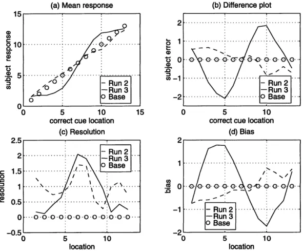
Data was averaged across all 8 sessions for each subject to find the statistics below. The resulting values were then averaged across all 5 test subjects to yields the data plotted in figures 2 through 9. Graphs were made for run-pairs corresponding to changes in warp strength (figs 5-1, 5-3, 5-5) and to the beginning and end of a warp (figs 5-2, 5-4, 5-6).

5.1

Mean Response

The mean response graphs (figs. 5-1, 5-2, 5-3, 5-4, 5-5, 5-6; panel a) plot correct versus subject response, where correct cue refers to the location to which the experiment trains the subject, and subject response is the (average) response given by subjects when presented with the associated correct cue. If all of a subject's responses are correct, the mean response line will fall exactly on the "correct answer" base line.

On run 3 (n = 1 to n = 4; fig 5-1a) subject overestimation produces a sigmoidal

response curve as a function of cue location. Over time (trial 3 to trial 17; fig 5-2a), subjects are able to partially adapt, indicated by a response curve closer to the base line response.

Comparing runs 17 and 18 (n = 4 to n = 2; fig 5-3a) we see that subjects adjust

quickly to the weaker transformation. The mean curve for run 18 is very close to the "correct answer" base line.

Continued training on the n = 2 cues (runs 18 to 32; fig 5-4a) produces slight improvement across all cues.

On the final change of cues (between runs 32 and 33, n = 2 to n = 1; fig 5-5a)

subject responses show underestimation similar to the change introduced between run 17 and 18. Consistent with previous runs, continued exposure improves subject performance (runs 33 to 40; fig 5-6a).

5.2

Error

Error (figs. 5-1 to 5-6; panel b) graphs show the difference between subject response and the correct response (noted as subject error). It is the inverse of the bias graphs with the exception of an inversion and normalization by the standard deviation.

Error is closely related to bias since it is equal to the error multiplied by -1 and divided by the standard deviation in subject responses. Thus, patterns in error can be understood by reading the discussion of bias results.

5.3

Resolution

The resolution (d') between location i and i + 1 is defined as

di+, mi+ - mi

where mi is the mean subject response for cue location i and ai is the standard deviation of the subject response to location i. Resolution measures a subject's per-ceived distance between adjacent cue locations normalized by the standard deviation in subject responses, and thus, measures the ability to discriminate between differ-ent sound sources. The perceptually closer the sources are to each other, the more difficult it becomes to discern them as separate locations, leading to lower values of resolution.

from n = 1 (run 2) to n = 4 (run 3). Under n = 4, the average distance between the normal cues just ahead of the subject (cue locations 5 through 9) increases, producing the expected improvement in resolution. With greater separation between

the forward-located cues (depicted in fig 3-1a: n = 1, and 3-1c: n = 4), they become

easier to resolve. Conversely, because the cues at the edges of the test range become more closely located, resolution begins to suffer.

Resolution decreases somewhat as exposure to the warped cues continues between runs 3 and 17 (fig 5-2c).

On the change from n = 4 (run 17) to n = 2 (run 18), center resolution degrades.

Center cue locations for n = 2 are spaced more closely than the cue locations for

n = 4 (compare figure 3-1c with 3-1b) producing the expected degradation in

resolu-tion. Larger spacing for locations at the edges of the range generate small resolution improvements in resolution beyond source locations 5 through 9. Continued expo-sure to n = 2 cues (runs 18 through 32; fig. 5-4) degrades resolution performance, if anything.

Upon returning to normal cues (runs 32 to 33; fig. 5-5) little change is seen in resolution. With continued exposure to the normal cues (runs 33 through 40; fig. 5-6), resolution remains relatively constant.

5.4

Bias

The bias 3 associated with cue i is

iz- mi o1i

Bias is a noise-adjusted measure of the error in subject response for a given source position, thus reflecting a subject's error in location as measured in units of response standard deviation.

For example, when subjects are initially exposed to more-strongly-warped cues

(except at the edges; see Impact of the edges). A simple estimate of bias for sudden changes in warping (ie, from run 2 [n = 1] to run 3 [n = 4] or run 17 [n = 4] to run 18 [n = 2]) can be found by subtracting the corresponding normal positions from the correct position (i.e., subtract fig 3-1a from fig 3-1c to generate crude bias values for

n = 1 to n = 4).

For cues with a weak to strong change (increasing warp n), an after-effect is caused by subject's overestimation of cue locations. On run 3, the subject first experiences warp n = 4. Assuming that he has adapted to n = 1 (which are normal cues and do not require adaptation; see section Imperfection in auditory cues), then his first exposure to n = 4 will produce responses in which he interprets the physical

stimuli like there is no transformation (n = 1). Looking at table 3.1, cue 81n=4 maps

approximately halfway between cue 101,=1 and cue 111n=1 (say 10.51,=1) and cue 91n=4 maps to cue 12.51,=1. The new mapping (n = 4) produces an overestimation which is consistent with the data. Additionally, larger shifts in cue remapping leads to greater overestimation which is also consistent with the data in the panel.

Figure 5-2d depicts the results for the 3rd to the 17th runs corresponding to the 1st and 15th runs with n = 4. Over time there is a decrease in average bias as subjects adapt to the cue transformation.

Conversely, for cues which change from strong to weak (decreasing warp n), sub-jects generally underestimate the cue locations. On run 18, subsub-jects are exposed to a warp n = 2 that is weaker than the most recent warp (n = 4). In this case, cue 91n=2

maps to cue 81n=4 and cue 131n=2 maps to cue 111n=4. Figure 5-3d results show the

expected underestimation caused by decreasing warp strength.

Figure 5-4d shows the 1st and 15th exposure to warp n = 2; again bias decreases over time.

On run 33, underestimation results when the subject is reintroduced to normal

cues n = 1 (down from n = 2) where, from table 3.1, cue 131n=1 maps to cue 111n=2

and cue 91n=1 maps to cue 81n=2 (fig. 5-5d). Because the magnitude of the location shifts are not as drastic as the initial change of n = 1 to n = 4, the magnitude of the error is not as great.

Figure 5-6 shows the 1st and 8th runs following the return to normal cues. In each case where the cues change (e.g., figures 5-1, 5-3, and 5-5), the correspond-ing change in bias is not as large as the differences reflected in table 3.1. Subject training is a continuous process throughout each run, and thus errors made early in the run may be larger than the errors later in the run (which may be reduced by adjustments made later in the run). Additionally, subjects are notified each time a cue is changed, and across the multiple sessions a subject participates in, he may be able to anticipate the new cues as soon as they are presented. Finally, subjects may not be completely adapted to the previous transformation when the cues are changed, resulting in a smaller than predicted change in bias. Even with these circumstances, data still strongly reflects the systematic over- and under-estimation consistent with adaptation (though imperfect) to each new cue transformation.

(a) Mean response 2 1 0 a -1 -2

correct cue location (c) Resolution

location

correct cue location

(d) Bias

0 5 10

location

Figure 5-1: Runs 2 and 3: Changing from n =

10

-o

-

Run

2

oo•

_{-Run 3}

0 0 Base

|

.o o.- o.- 0. o o o o0oo.0

...

... ...

... I

"

... ...

_B

_ase

-

Run 2

...

..-

...-

o....

...

...

. ...

...

...

...

...

..

· · ·

...

..

(a) Mean response

5 10

correct cue location (c) Resolution 5 10 location 2 1 U) -1 -2 1 A 0 -1 (b) Difference plot / ,',0, 0_ 0-, 0-00

- Run 3

correct cue location

(d) Bias

0

location

Figure 5-2: Runs 3 and 17: Start and finish of n = 4

15 CD o10 u) U) .LJ 2.5 2 1.5 1 0.5 0 -0.5 / : - Run 3 / -Run 17 ... .... o Base

o.i0.-0.

o00

.0

o..

. : : /..

S/'

a m

(a) Mean response

correct cue location (c) Resolution

0 5 10

correct cue location

(d) Bias 2.5 2 1.5 1 0.5 0 -0.5 location 0 5 location 10

Figure 5-3: Runs 17 and 18: Changing from n =

5 0 5 1 u) C ol 0. a, 0) a, a, O ... -Run 1' -Run 1] o Base f \ -Run 17 ... ... _{-- Run 18} \ o Base

.

..

...

...

.

...

.... .

....

....

...

..

(a) Mean response

correct cue location (c) Resolution 2 1 0 C, )-I -2 C 5 10

correct cue location

(d) Bias

location location

Figure 5-4: Runs 18 and 32: Start and finish of n = 4

- Run 18 - Run 32 o B ase ... 2.5 2 1.5 1 0.5 0 -0.5

0

-(a) Mean response

5 10

correct cue location (c) Resolution - Run 32 -Run 33 i oBase .. ... O O.. ... ... ... . .... ... 0 00 0-"0" 0-0-"-location 2 1 S-1 -2 (b) Difference plot ... ... ...

-Run 33

..

...

0

B

ase

...

correct cue location

(d) Bias 1 ._ 0 .0 -1 0r 0 5 location

Figure 5-5: Runs 32 and 33: Changing from n = 2 to n = 1

15 a) io 010 W. CD (I 1.5 1 0.5 - Run 32 -Run 33 o Base

.o

,6 o

-

.0.

0--o

o 0

..

.."..

....

...

...

(a) Mean response

correct cue location (c) Resolution

(b) Difference plot

0 5 10

correct cue location (d) Bias 02 location -0 location

Figure 5-6: Runs 33 and 40: Start and finish of n = 1

o 10 0. t5 CD Ar 0

;

..

...

...

...

ar

.9'.>

.

.

.

.

-....

. . .

5.5

Estimating Adaptation

The degree of adaptation can be measured by the slope of the line that best fits mean response as a function of 0', the normal position of the stimuli. Observation of subject response versus normal cue location (figure 8) show that response has a

roughly linear shape as a function of 0'. From start to finish of n = 4 exposure (runs

3 and 17, respectively; figs. 5-7a and 5-7b) and from start to finish of n = 2 (runs

18 and 32, respectively; figs. 5-7c and 5-7d) the subject response as a function of normal cue appears linear. However, the slope of the line relating mean response to 0' changes over time.

The best-fit was generated by finding the line that minimizes the mean-square error between predicted and measured subject response. Because the correct cue for ahead (light 7) remains the same as the normal cue location for straight-ahead, each line-fit was forced to contain the point where normal cue straight-ahead is the same as subject response straight-ahead (i.e., only the slope of the line changed; the intercept was assumed fixed).

Because some warp levels generate cues that fall outside of the normal response range, only normal cues that fall between +60 and -60 degrees are considered. For

example, when the warp level changes from n = 1 to n = 4, cue 21n=4 is presented

from -78 degrees and due to his familiarity with the n = 1 space, the best the subject

can respond with is location 1. Rather than make assumptions about the adaptation

patterns, cues whose normal locations are outside of the normal response range (n = 1;

+60 to -60) are left off of adaptation calculations (see Impact of the edges).

These line-fit results were compared to a transform-fit approach. Rather than finding the best-fit slope of a line, the subject responses were fitted by varying the warp strength, n, in the transform formula (given on page 7). Tabulation of the mean-square error on a run-by-run basis (tables A.1 and A.2) showed that the line-fit is generally better than the warp-fit. In runs where the warp-fit produced better error results, the difference is very small (i.e., runs 33 to 40).

(b) Run 17 0 5 10 15 normal location (c) Run 18 12 2 10 0 0. a 8 5 6 CD ₄ 2 0 12 C 10 a 8 6 4

2

Figure 5-7: Observation of linearity

0 5 10 normal location : : : ... ... ... ...._{...... . ...}

.

.

.

.

.

.

.

.

.

.

.

.

.

.

.

.

.

.

.

.

.

.

..

.

.

.

.

.

.

.

.

...

.

.

.

.

.

.

.

.

.

.

.

.

.

.

.

.

.

.

.

.

.

.

.

.

.

.

.

.

..

...

Individual results are presented in figure 5-8. Rates and asymptote values vary across subjects and are summarized in table 5.1. Rate is the time constant associ-ated with the exponential valued in terms of runs. Subject responses that could not successfully fit an exponential are listed as N/A.

Comparing subjects, we see that all five subjects appear to adapt to the n =

4 transformation at roughly the same rate. However, it is clear that the rate of

adaptation can vary greatly between subjects when changing from strong (n = 4)

to weak (n = 2) transformations. For instance, subject LCW adapts slowly to the

n = 2 transformation when compared to subject JJP. In contrast, two subjects (MSS

and SC) appear to show no change in slope during exposure to n = 2 cues (note the

flat line fit to their data in runs 17 through 32); instead, their performance is stable throughout this exposure period.

subject JJP JIR LCW MSS SC runs 3-17 asymptote 0.55 0.62 0.60 0.61 0.66 rate 0.71 0.89 1.20 1.05 0.69 runs 18-32 asymptote 0.64 0.70 0.68 0.67 0.72

rate 0.99 3.77 6.17 N/A N/A

runs 33-40

asymptote 0.87 0.85 0.84 0.83 0.89

rate 1.44 3.10 1.68 2.34 N/A

Table 5.1: Subject Exponential Fit Results

Subject: MSS Subject: LCW 10 Subj2c: JIR 30 10 _{Subject: SC}20 30 00.9 o 0.8 0.7 S0.6 0.5 0 00.9 o 0.8 0.7 S0.6 0.5 0 10 .20 ... 30 Subject: JJP 10 20 30 10 20 30 40

Figure 5-8: Individual Adaptation Results

0.9 O 0.8 S0.7 Q0.6 0.5 0 h : 0.9 0.8 0.7 0.6 (c . . 0 0.9. 0.8 0.7 0.6 (d)

...

'

''''''

I

Figure 5-9 plots the best-fit line slope averaged across the five subjects as a func-tion of run. It appears that the best-fit slope changes gradually when cue trans-formation changes. Consistent with [1], the average slope appears to exponentially approach an asymptotic value as the subjects adapt to each transformation. Given the inter-subject differences in adaptation rate, little can be said about the relative

rate of adaptation from n = 1 to n = 4 compared to adapting from n = 4 to n = 2.

But, the rate of adaptation is roughly consistent with the average rate of adaptation in previous experiments [1].

The average asymptote of adaptation across subjects when n = 4 is 0.61 (with

a standard deviation of 0.04) and roughly 0.68 (with a standard deviation of 0.03)

when n = 2. These values are comparable to the average values for asymptotes of

previous experiments where n = 4 (asymptote of 0.59 with a standard deviation of

0.07) and n = 2 (asymptote of 0.73 with a standard deviation of 0.04) [1] especially

Adaptation 0.95 0.9 0.85 0.8 0 1-i 0.75 0.7 0.65 0.6 055155 0 2 0 5 10 15 20 25 runs

Figure 5-9: Adaptation over runs

5.6

Imperfection in auditory cues

The unwarped HRTFs used in the experiment are based on measurements taken by Wightman [3] from the subject SDO, a petite female. Because of the original subject's smaller head, subject interpretation of the audio cues are slightly skewed. The error introduced is predictable and can be accounted for by considering the effects of only the ITD associated with the HRTF.

For some angle 0 there is an associated ITD(O) for each subject. Assuming that

Wightman's subject SDO has a head smaller than any subject I use, interaural delays presented to my subjects will be smaller than normal for a source at a particular position. That is, angle Ox normally gives rise to ITDSDo(Ox) and ITDtestsubject(Ox) where, generally

IITDsDo(Ox)I < IITDtest-subject (Ox)

because of SDO's smaller head. When a source from Ox is presented, even for normal

cues (n = 1), the subject will perceive the source to be at some position lal < OxlJ

While this analysis explains systematic errors in localization (whereby the mag-nitude of the source angle is underestimated) for normal cues, these errors are very small compared to the errors introduced when the auditory cues are transformed (fig. 2-1).

5.7

Impact of edges

Data at the extremes of the testing range must be handled differently. For example,

between the second and third runs where the cues change from n = 1 to n = 4, the

auditory range changes from +60 to -60 when n = 1 to +82 to -82 when n = 4.

Because of this change, the range of auditory cues exceeds the range of possible response positions whenever n > 1.

Because subjects are not instantly familiar with the transformed auditory space, they are forced to interpret the cues in the context of the old auditory space. When

instance, with n = 4 the normal cues for auditory sources 1 through 4 and 10 through 13 fall outside the range of responses (+60 to -60 degrees). Under the expanded range, it is likely that when the subject initially hears any cue less than 5 or greater than 9, they will answer 1 or 13, respectively. The difference plot in figure 5-1b, for example, reflects this effect by the sudden decrease in error occurring before cue 4 and after cue 10. The small error at the extremes result from the fact that the response range available to the subjects limits the errors possible at the edge of the range.

To minimize error introduced by these edges, the edge data is treated differently in the calculation of adaptation.

Chapter 6

Summary

Over the two-hour test period, subjects are able to adapt to the various changes in-troduced into their auditory environment. Error and bias plots show systematic error and adaptation. Errors and bias values always decreases as exposure to a particular warp-strength continues. The mean graphs also demonstrate adaptation as subject response consistently shifts towards the base line.

Other indications of adaptation are demonstrated by systematic over- and under-estimation at instances where warp strength changes. A weak to strong cue change (run 2 to run 3) produces an overestimation of cue distance from the center while weak to strong cue changes (run 17 to run 18 and run 32 to run 33) lead to underestimation of cue locations with respect to the center.

Adaptation can be summarized by the slopes of the line generated by normal cue versus subject response. In this experiment, adaptation happens at a rate comparable to adaptation seen in previous experiments when changing from a weak to a strong

warp (n = 1 to n = 4), but is inconsistent across subjects when changing from strong

to weak transforms (n = 4 to n = 2 and n = 2 to n = 1). This difference may be the

result of the magnitude of the change or the direction of the change.

A previous model of adaptation [1] predicts that the exponential rate of adaptation is independent of the order of runs. Current results are consistent with this prediction for the initial change in transformation, but show that subject differences can occur with subsequent cue changes. The same model predicts that the asymptote to which

subjects adapt depends only on the transform strength. The asymptote values in current experiments are quantitatively consistent with this model.

Appendix A

run fit-value 0.915000 0.876000 0.688000 0.641000 0.621000 0.617000 0.609000 0.612000 0.604000 0.609000 0.632000 0.608000 0.594000 0.606000 0.602000 0.591000 0.592000 0.651000 0.657000 0.654000 0.671000 0.665000 0.673000 0.661000 0.673000 0.678000 0.679000 0.683000 0.680000 0.674000 0.701000 0.691000 0.777000 0.805000 0.820000 0.834000 0.848000 0.852000 0.866000 0.853000

Table A.1: Line-Fit values

MSE 0.062621 0.041815 0.139680 0.137652 0.143011 0.163654 0.162175 0.169945 0.221647 0.256640 0.198166 0.315373 0.341567 0.299267 0.300367 0.467556 0.186458 0.216157 0.147900 0.143736 0.188446 0.205563 0.138698 0.166358 0.166455 0.158415 0.132656 0.176875 0.177086 0.133242 0.186548 0.158317 0.155936 0.114007 0.072180 0.070147 0.055556 0.055053 0.065929 0.058607

fit-value run 0.875000 0.810000 1.555000 1.310000 1.215000 1.210000 1.175000 1.185000 1.160000 1.175000 1.275000 1.180000 1.120000 1.160000 1.150000 1.110000 1.110000 0.855000 0.890000 0.880000 0.920000 0.905000 0.930000 0.900000 0.925000 0.940000 0.935000 0.945000 0.945000 0.930000 0.995000 0.965000 0.755000 0.755000 0.755000 0.755000 0.770000 0.775000 0.795000 0.780000

Table A.2: Warp-Fit Values

MSE 0.076250 0.034485 1.976269 1.627068 1.313647 1.499365 1.359899 1.357868 1.529519 1.303260 1.545372 1.494498 1.215115 1.232352 1.255091 1.184178 1.248420 0.174047 0.181483 0.154377 0.166857 0.127646 0.228298 0.190203 0.144188 0.219329 0.098412 0.134091 0.214962 0.155193 0.204137 0.175897 0.150068 0.079870 0.044412 0.052217 0.035308 0.037839 0.057732 0.047575

Bibliography

[1] Barbara G. Shinn-Cunningham. Supernormal Auditory Localization Cues in an

Auditory Virtual Environment. PhD thesis, Massachusetts Institute of Technology,

1994.

[2] Elizabeth M. Wenzel. Localization in virtual acoustic displays. Presence, 1(1):80-107, 1992.

[3] F.L. Wightman and D.J. Kistler. Headphone simulation of free-field listening.