HAL Id: hal-00437304
https://hal.archives-ouvertes.fr/hal-00437304
Submitted on 30 Nov 2009
HAL is a multi-disciplinary open access
archive for the deposit and dissemination of
sci-entific research documents, whether they are
pub-lished or not. The documents may come from
teaching and research institutions in France or
abroad, or from public or private research centers.
L’archive ouverte pluridisciplinaire HAL, est
destinée au dépôt et à la diffusion de documents
scientifiques de niveau recherche, publiés ou non,
émanant des établissements d’enseignement et de
recherche français ou étrangers, des laboratoires
publics ou privés.
To cite this version:
Thanh Phuong Nguyen,
Isabelle Debled-Rennesson.
On the local properties of digital
curves. International Journal of Shape Modeling, World Scientific Publishing, 2008, pp.105-125.
�10.1142/S0218654308001105�. �hal-00437304�
c
° World Scientific Publishing Company
On the local properties of digital curves†∗
Thanh Phuong Nguyen‡and Isabelle Debled-Rennesson
LORIA, Campus Scientifique - BP 239, 54506 Vandoeuvre-l`es-Nancy Cedex, France {nguyentp,debled}@loria.fr
We propose a geometric approach to extract local properties of digital curves. This approach uses the notion of blurred segment1 that extends the definition of segment of arithmetic discrete line2 to adapte to noisy curves. A curvature estimator3 for 2D curves in O(n log2n) time is proposed relying on this flexible approach. The notion of 2D blurred segment is extended to 3D space. A decomposition of the curve into 3D blurred segments is deduced and allows new curvature and torsion estimators for 3D curves. All these estimators can naturally work with disconnected curves.
Keywords: curvature, torsion, digital curve, discrete line, blurred segment
1. Introduction
Geometric properties of curves are important characteristics to be exploited in ge-ometric processing. They directly lead to applications in machine vision, computer graphics. So curvature for 2D curves, curvature and torsion for 3D curves are in-teresting subjects to study digital curves.
In the 2D case, many applications are based on the curvature property in
do-mains such as curve approximation4, geometry compression5, and particularly in
corner detection after the pioneer paper of Attneave 6. Curvature estimation is a
key problem for many applications in image processing that require the geometric measures of represented discrete objects.
In 3D space, torsion and curvature are the most important properties that per-mit to study the bending of a spatial curve. Several methods have been proposed
for torsion estimation. Mokhtarian 7 used Gaussian smoothing to estimate torsion
directly with a torsion formula. Similarly, Kehtarnavaz et al.8used B-spline
smooth-ing techniques; Lewiner et al. 5proposed weighted least-squares fitting techniques.
Raluben Medina et al. 9 proposed two methods to estimate torsion and curvature
values at each point of the curve. The first used the Fourier transform, the second is based on the least squares fitting. These methods are applied in the description of arteries in medical imaging.
In the framework of the discrete geometry, estimators of geometrical parameters have been proposed, but these methods rely on the recognition of discrete line ∗This work is supported by ANR in the framework of the GEODIB project, BLAN 06 − 2 134999. †Based on ”Curvature Estimation in Noisy Curves” and ”Curvature and Torsion Estimators for 3D Curves” by T.P. Nguyen and I. Debled-Rennesson respectively in proceedings of CAIP’07 and ISVC’08.
‡Corresponding author
segments which is very sensitive to the noise present in the studied curves10,11,12.
The boundary of discrete objects is often noisy due to the acquisition process.
Therefore the concept of blurred segment was introduced1, which allows the flexible
segmentation of discrete curves, taking noise into account. Relying on an arithmetic
definition of discrete lines2, it generalizes such lines, admitting that some points
are missing.
We propose in this paper a novel method, based on the definition of blurred segments, for the estimation of local geometric parameters of 2D and 3D curves. It uses a geometrical approach and relies on results of discrete geometry on
de-composition of a curve into maximal blurred segments 10,1,3. This paper recalls
the obtained results for a 2D curvature estimator3 and presents an extension to
3D of these results. The 3D curvature estimator given in13 is extended with the
notion of blurred segment and permits to study noisy or disconnected curves. We also propose a new approach to the discrete torsion estimation.
The paper is organized as follows. In Section 2, after recalling some definitions related to 2D blurred segments, we study the problem of adding (or removing) a point to (from) a 2D blurred segment of width ν in the case of general discrete curves. Then we propose an extension for noisy curves the notion of maximal seg-ment of a discrete curve. An algorithm to determine all maximal blurred segseg-ments of a 2D discrete curve is given in Section 3. In Section 4, after recalling the defini-tion of the curvature estimator adapted to 2D noisy curves, an algorithm for the determination of the curvature at each point of a discrete curve is proposed. In this section, we also present how to extend these ideas into the 3D space. The next sections propose curvature and torsion estimators for 3D curves. The last section gives experiments and comparisons with Mokhtarian’s and Lewiner’s methods.
2. Blurred segment of width ν 2.1. Definitions
2.1.1. 2D case
The notion of blurred segments relies on the arithmetical definition of discrete
lines 2. A line, with slope a
b, lower bound µ and thickness ω (with a, b, µ and ω
being integer such that gcd(a, b) = 1) is the set of integer points (x, y) verifying
µ≤ ax−by < µ+ω. Such a line is denoted by D(a, b, µ, ω). Let us recall definitions1
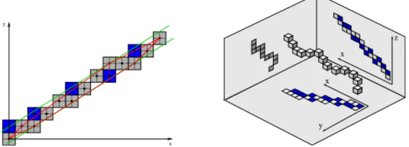
that we use in this paper (see Fig. 1.a):
Definition 2.1. Let us consider a set of 8-connected points Sb. The discrete line
D(a, b, µ, ω) is said bounding for Sb if all points of Sb belong to D.
Definition 2.2. Let us consider a set of 8-connected points Sb. A bounding line
of Sb is said optimal if its vertical distance (i.e. max(|a|,|b|)ω−1 ) is minimal, i.e. if its
vertical distance is equal to the vertical distance of conv(Sb), the convex hull of Sb.
Definition 2.3. A set Sb is a 2D blurred segment of width ν if its optimal
bounding line has a vertical distance less than or equal to ν i.e. if ω−1
max(|a|,|b|) ≤ ν.
A linear recognition algorithm of the 2D blurred segment of width ν is proposed in1.
y x x z x y
Fig. 1. From left to right: a. D(5, 8, −8, 11), optimal bounding line (vertical distance =
10
8 = 1.25) of the sequence of gray points - b. D3D(45, 27, 20, −45, −81, 90, 90) optimal
discrete line of the grey points.
2.1.2. 3D case
The notion of 3D discrete line (see the14,15) is defined as follows:
Definition 2.4. A 3D discrete line [43], denoted D3D(a, b, c, µ, µ′, e, e′), with a
main vector (a, b, c) such that (a, b, c) ∈ ZZ3, and a ≥ b ≥ c is defined as the set of
points (x, y, z) from ZZ3verifying:
D½ µ ≤ cx − az < µ + e (1)
µ′ ≤ bx − ay < µ′+ e′ (2)
with µ, µ′, e, e′∈ ZZ. e and e′ are called arithmetical width of D.
According to the definition, it is obvious that a 3D discrete line is bijectively projected into two projection planes as two 2D arithmetical discrete lines. Thanks to that property, we naturally define the notion of 3D blurred segment by using the notion of 2D blurred segment and by considering the projections of the sequence of studied points in the coordinate planes (see Fig. 1.b)
Definition 2.5. Let Sf3D be a sequence of points of ZZ3, Sf3D is a 3D blurred
segment of width ν with a main vector (a, b, c) such that (a, b, c) ∈ ZZ3, and
a≥ b ≥ c if it possesses a said optimal discrete line, named D3D(a, b, c, µ, µ′, e, e′),
such that
• D(a, b, µ′, e′) is optimal for the sequence of projections of points of Sf
3D
in the plane (O, x, y) and e′−1
max(|a|,|b|) ≤ ν,
• D(a, c, µ, e) is optimal for the sequence of projections of points of Sf3D in
the plane (O, x, z) and e−1
max(|a|,|c|) ≤ ν.
A linear algorithm of 3D blurred segment recognition may be deduced from that definition. Indeed, we only need to use an algorithm of 2D blurred segment
2.2. Add (or remove) a point to (from) a 2D blurred segment of width ν
In this section we study the problem of adding (or removing) a point to (from) a blurred segment of width ν. The recognition algorithm of 2D width ν blurred
segments presented in1 is executed in linear time. However, it only considers the
incremental addition of a point to a blurred segment in the first octant. We present here the general case which requires the incremental calculation of both height and width of the convex hull after adding or removing a point. To do that, we use the
results given in16and17 that we briefly recall below.
Dynamic estimation of the convex hull:
The problem of dynamic estimation of the convex hull of a set of points when adding (or removing) a point to (from) this set was proposed by M.H. Overmars and J. van
Leeuwen16. The convex hull is represented by Concatenable Queue data structure
that support search, insert, removal, split and concatenate operations in O(log n)
time18. A segment tree data structure was proposed to allow to work with convex
hull based on the divide-and-conquer strategy. This strategy is based on the fact: it costs O(log n) time to determine the bridge between 2 convex hulls. In their work,
a convex hull is considered as the union of two parts: the upper convex hull (Uhull)
and the lower convex hull (Lhull) which correspond to 2 segment trees. They are
updated after each operation of addition or removal of a point. The cost of these
operations are estimated by the following theorem16.
Theorem 1. The convex hulls Uhull and Lhull of the set S of n points may be
dynamically kept, in the worst case, in O(log2n) by an operation of addition or
removal.
Determination of height and width of the convex hull:
We use the double technique of binary search17to determine the height and width
of the convex hull. In 17, the convex hull is also considered as the union of two
parts Uhull and Lhull. The double technique of binary search permits to find the
vertical width of the convex hull by using the concavity property of the function
height(x) = Uhull(x) − Lhull(x) in O(log2n). To do that, firstly, for each point in
the upper convex hull, he applied binary search technique to detemine its opposite edge on the lower convex hull. So the height from this point to the lower hull is determined. By applying one time the binary search technique on the upper convex hull, the maximal height between the upper and lower convex hulls will be
determined. So, the complexity of this double technique is O(log2n).
3. Maximal blurred segment of width ν 3.1. Definitions and first proposition
The notion of the maximal segment of a discrete curve was proposed in10,12 and
relies on the discrete line segments. This structure enables a global understanding of the discrete curve to be analyzed. We propose here an extension of that notion
to blurred segments, adapted to noisy curves, by using the same notation as in12.
Let us consider a 2D or 3D discrete curve called C, the points of C are indexed from 0 to n − 1. C is a general curve and the points of C can be
discon-nected . We note Ci,ja set of successive points of C ordered increasingly from index
ito j.
by BS(i, j, ν). The first index j, i ≤ j, such that BS(i, j, ν) and ¬BS(i, j + 1, ν) is called the front of i and noted F (i). Symmetrically, the first index i such that BS(i, j, ν) and ¬BS(i − 1, j, ν) is called the back of j and noted B(j).
Definition 3.2. Ci,j is called a maximal blurred segment of width ν and
noted M BS(i, j, ν) iff BS(i, j, ν) and ¬BS(i, j + 1, ν) and ¬BS(i − 1, j, ν). It is obvious that an equivalent characterization for a maximal blurred segment of width ν, M BS(i, j, ν), is to show that F (i) = j and B(j) = i. In this work, we use the notion of blurred segment of width ν which is maximal on the right or on the left sides:
Definition 3.3. Ci,j is called a maximal blurred segment of width ν on the
right side (resp. on the left side) and noted M BSR(i, j, ν) (resp. M BSL(i, j, ν))
if F (i) = j (resp. B(j) = i).
Proposition 1. Let C be a discrete curve, M BSν(C) the sequence of maximal
blurred segments of width ν of the curve C. Then, M BSν(C) = {M BS(B1, E1, ν),
M BS(B2, E2, ν), ..., M BS(Bm, Em, ν)} and satisfies B1 < B2 < ... < Bm. So we
have: E1< E2< ... < Em.
Proof: We consider 2 consecutive maximal blurred segments M BS(Bi, Ei, ν) and
M BS(Bi+1, Ei+1, ν). By hypothesis, Bi < Bi+1, let us suppose that Ei >
Ei+1, then M BS(Bi+1, Ei+1, ν) becomes a part of M BS(Bi, Ei, ν). Therefore
M BS(Bi+1, Ei+1, ν) is not a maximal blurred segment, which is contradictory.
3.2. Algorithm for the segmentation of a curve C into maximal blurred segments
3.2.1. 2D case
We propose the algorithm 1 which determines all maximal blurred segments of width ν of a 2D discrete curve C according to the conditions given in section 3.1 by using proposition 1.
Complexity
Each point of the curve is scanned at most twice in this algorithm. The cost of determining a new optimal bounding discrete line when we add (or remove) a point
to (from) a blurred segment is in O(log2n). Hence the complexity of this algorithm
is in O(n log2n).
3.2.2. 3D case
The algorithm 2 permits to obtain the sequence of 3D maximal blurred segments of
width ν in time O(n log2n) for any noisy 3D discrete curve C. It uses the algorithm 1
to determine the 2D maximal blurred segments of the projections in the coordinate planes of the points of the studied curve.
To determine the optimal discrete line of the current 3D blurred segment Sb
(step marqued with (*) in the algoritm 2), we consider the characteristic of the two 2D blurred segments obtained in the planes of projection and combine them
to obtain the characteristics of the optimal 3D discrete line of Sb. As the whole
process is done in dimension 2, this algorithm 2 has the same complexity as the one in dimension 2. So, we have the theorem below.
Algorithm 1: Algorithm for the segmentation of a curve C into 2D maximal blurred segments of width ν
Data: C - discrete curve with n points, ν - width of the segmentation Result: M BSν - the sequence of maximal blurred segments of width ν
begin k=0; Sb= {C0}; M BSν= ∅; a = 0; b = 1; ω = b, µ = 0; while maxω−1 (|a|,|b|)≤ ν do k++; Sb= Sb∪ Ck; Determine D(a, b, µ, ω) of Sb; bSegment=0; eSegment=k-1 ; M BSν = M BSν∪ M BS(bSegment, eSegment, ν); whilek < n− 1 do while max(|a|,|b|)ω−1 > ν do Sb= Sb\ CbSegment; bSegment++ ;
Determine D(a, b, µ, ω), optimal bounding line of Sb; while ω−1
max(|a|,|b|)≤ ν do
k++ ; Sb= Sb∪ Ck;
Determine D(a, b, µ, ω), optimal bounding line of Sb;
eSegment=k-1; M BSν= M BSν∪ M BS(bSegment, eSegment, ν);
end
Algorithm 2: Algorithm for the segmentation of a curve C into maximal 3D
blurred segments of width ν
Data: C - discrete curve with n points, ν - width of the segmentation Result: M BSν - the sequence of maximal blurred segments of width ν of C
begin
k=0; Sb= {C0}; M BSν= ∅; a = 0; b = 1; ω = b, µ = 0;
whilethe widths of 2 blurred segments obtained by projecting the points of Sb in the coordinate planes are≤ ν do
k++; Sb= Sb∪ Ck ;
Determine D3D(a, b, c, µ, µ′, e, e′), optimal discrete line of Sb; (*)
bSegment=0; eSegment=k-1 ;
M BSν = M BSν∪ M BS(bSegment, eSegment, ν);
whilek < n− 1 do
whilethe widths of 2 blurred segments obtained by projecting the points of Sb in the coordinate planes are > ν do
Sb= Sb\ CbSegment; bSegment++ ;
Determine D3D(a, b, c, µ, µ′, e, e′), optimal discrete line of Sb; (*)
whilethe widths of 2 blurred segments obtained by projecting the points of Sb in the coordinate planes are≤ ν do
k++ ; Sb= Sb∪ Ck;
Determine D3D(a, b, c, µ, µ′, e, e′), optimal discrete line of Sb; (*)
eSegment=k-1; M BSν= M BSν∪ M BS(bSegment, eSegment, ν);
Theorem 2. The decomposition of a 3D curve into maximal blurred segments of
width ν can be done in time O(nlog2n).
4. Discrete curvature of width ν 4.1. Definition
We recall here the curvature estimator which is adapted to noisy curves 19. It is
directly deduced from the estimator proposed by D. Coeurjolly 11 for 2D curves
without noise. This technique can be seen as a generalization of the classical order
m normalized curvature20. Let C be a 2D or 3D discrete curve, C
k is a point of the D(1,−2,−3,5) D(1,2,−2,5) Ox Oy Radius: 14.7638 Ck CR CL (a)
B
iB
i+1E
i+1E
i (b)Fig. 2. a. Estimation of the 2D curvature at the point Ck with width 2; b. Ei (Bi+1) is front (back) of points in first (second) bold edge.
curve. Let us consider the points Cl and Crof C such that : l < k < r, BS(l, k, ν)
and ¬BS(l − 1, k, ν), BS(k, r, ν) and ¬BS(k, r + 1, ν).
The estimation of the curvature of width ν at the point Ck shall be
de-termined as the inverse of the radius of the circle passing through the points Cl,
Ck and Cr. To determine the radius Rν(Ck) of the circumcircle of the triangle
[Cl, Ck, Cr], we use the formula given in21 as follows (see Fig. 2.a and Fig. 3).
Let s1= || −−−→ CkCr||, s2= || −−−→ CkCl|| and s3= || −−−→ ClCr||, then Rν(Ck) = s1s2s3 p(s1+ s2+ s3)(s1− s2+ s3)(s1+ s2− s3)(s2+ s3− s1)
Then, the curvature of width ν at the point Ck is Cν(Ck) = Rν(Cs k) with s =
sign(det(−−−→CkCr,
−−−→
CkCl)) (it indicates concavities and convexities of curve).
As indicated in 11, the degenerated cases, which correspond for example to
colinear half-tangents, may be independently tested and, thus, a null curvature is affected to the considered point.
4.2. Estimation of the curvature of width ν at each point of C
In this section, we propose a new algorithm for the determination of the curva-ture of width ν at each of the n points of a 2D or 3D curve C. The complexity of
this algorithm is better than the one of the naive algorithm, in O(n2). It consists
of calculating at each point Ck, the maximal blurred segment on the right side,
passing through 3 points: (left extremity of M BSL, Ck, right extremity of M BSR).
Description of the algorithm (see Fig. 3)
Let M BSR(k, r, ν) and M BSL(l, k, ν) be the maximal blurred segments on the
right and left sides of the point Ck. Then, there exist r′ ≤ k and l′ ≥ k such that
M BSR(k, r, ν) ⊂ M BS(r′, r, ν) and M BSL(l, k, ν) ⊂ M BS(l, l′, ν).
Let us then consider the decomposition of C into maximal blurred segments:
M BSν(C) = {M BS(B1, E1, ν), M BS(B2, E2, ν), ..., M BS(Bm, Em, ν)} with B1<
B2< ... < Bm and E1< E2< ... < Em. We look for the indices i and j such that
iis the first index such that Ei ≥ k and j is the last index such that Bj ≤ k. So
it is obvious that l = Bi, r = Ej and that the curvature of width ν at the point
Ck is the inverse of the radius of the circumcircle of the triangle [Cl, Ck, Cr]. More
generally, we have the following result.
Definition 4.1. Let L(k), R(k) be the functions which respectively represent the indices of the left and right extremities of the maximal blurred segments on the left
and right sides of the point Ck.
• ∀k such that Ei−1< k≤ Ei, then L(k) = Bi
• ∀k such that Bi≤ k < Bi+1, then R(k) = Ei
This definition is used in the algorithm 3 (see also Fig. 2.b).
Algorithm 3:Width ν curvature estimation at each point of a 2D or 3D curve
Data: C Discrete curve of n points, ν width of the segmentation Result: {Cν(Ck)}k=0..n−1- Curvature of width ν at each point of C
begin
Build M BSν= {M BSi(Bi, Ei, ν)}i=0 to m−1(see Algorithm 1 for 2D case or
Algorithm 2 for 3D case); m = |M BSν|; E−1= −1; Bm= n;
fori= 0 to m − 1 do
fork= Ei−1+ 1 to Ei doL(k) = Bi;
fork= Bi to Bi+1− 1 do R(k) = Ei;
fori= 0 to n − 1 do
Rν(Ci) = Radius of the circumcircle to [CL(i), Ci, CR(i)];
Cν(Ci) =
sign(det(−−−−−→CiCR(i),−−−−−→CiCL(i)))
Rν(Ci) ;
end
Remark: The bounds mentioned in the algorithm 3 are correct for a closed curve. In the case of an open curve, the instruction becomes: for i = l to n - 1 - l with l fixed to a constant value. Indeed it is not possible to calculate a maximal blurred segment on the left side (resp. on the right side) at the first point (resp. at the last point) of the curve. Thus the calculation of the curvature begins (resp. stops) at
the lth(resp. (n − 1 − l)th) point of the curve.
Complexity
Both steps of labelling and estimation of the curvature at each point are executed in linear time. However, the determination of the maximal blurred segments are
executed in O(n log2n). Thus the complexity of our method is O(n log2n). Because
the complexity of a blurred segment is O(n) for simple curves, and O(n log n) for
complexity with simple curve and O(n2log n) for general curve. Let us recall that
a simple curve is a polygonal chain of line segments that do not cross each other. It is not correct for general curve. So, this algorithm is more efficient than existing method.
Fig. 3. Given a spatial curve, firstly the set of maximal blurred segments is computed. To determine the curvature value at the second black point, its left (resp. right) extremity is located as the left (resp. right) extremity of the corresponding maximal blurred segment, and then the curvature value is estimated as the inverse of circumcircle radius. Working width is 2.
5. Discrete torsion of width ν 5.1. Definitions
The curvature is not sufficient to characterize the local properties of a 3D curve. This parameter only measures how rapidly the direction of the curve changes. In case of a planar curve, the osculating plane does not change. For 3D curves, torsion is a parameter that measures how rapidly the osculating plane changes. To clarify this notion, we recall below some definitions and results in differential geometry
(see the22 for more details).
Definition 5.1. Let r : I → R3be a regular unit speed curve parameterized by t.
[i] T (t) (resp. N (t)) is a unit vector in direction r′(t) (resp. r′′(t)). So, N (t) is
a normal vector to T (t). T (t) (resp. N (t)) is called the unit tangent vector (resp. normal vector) at t.
[ii] k(t) = |T′(t)| is called the curvature of r at t.
[iii] The plane determined by the unit tangent and normal vectors (T (t) and
N(t)), is called the osculating plane at t. The unit vector B(t) = T (t) ∧ N (t) is
[iv] τ (t) = |B′(t)| is called the torsion of curve at t.
Definition 5.2. Let r : I → R3 be a spatial curve parameterized by t.
i The curvature of r at t ∈ I: k(t) =|r ′ ∧r′′| |r′ |3 ii The torsion of r at t ∈ I: τ (t) =(r ′ ∧r′′).r′′′ |r′ ∧r′′ |2
According to the definition 5.2, the torsion value at a point is 0 if the curvature value at this point is 0.
5.2. Discrete torsion
Discrete torsion was studied in5,7,9,8. In this section, we propose a new geometric
approach for the problem of torsion estimation that uses the definitions and results presented in the previous sections.
5.2.1. Definitions
Let ζ be a 3D discrete curve, Ck is kth point of the curve. Let us consider the
points Cl and Cr of ζ such that : l < k < r, BS(l, k, ν)&¬BS(l − 1, k, ν) and
BS(k, r, ν)&¬BS(k, r + 1, ν). Recall that the curvature of width ν is estimated
by circumcircle of triangle △ClCkCr. If
−−−→
CkCland
−−−→
CkCr are colinear, the curvature
value at Ck is 0, therefore the torsion value at Ck is 0. So, without loss of generality,
we suppose that −−−→ClCk and
−−−→
CkCr are not collinear. In addition, the plane defined
by−−−→ClCk and
−−−→
CkCr is noted (Cl, Ck, Cr), and we propose the definition below.
Definition 5.3. The osculating plane of width ν at Ckis the plane (Cl, Ck, Cr).
The osculating plane (Cl, Ck, Cr) has two unit tangent vectors : −→t1 =
−−−→ ClCk |−−−→CkCr| and − → t2 = −−−→CkCr |−−−→CkCr|
. Therefore, we have the binormal vector at the kthpoint:−→b
k =
− → t1 ∧−→t2 =
(bx, by, bz) So, we propose the following definition of discrete torsion of width ν.
Definition 5.4. The discrete torsion of width ν at Ck is the derivative of
− → bk.
5.2.2. Torsion estimator
Our proposed method for torsion estimation is based on the definition 5.4. Let us
remark that the set {−→bk}n−1k=0 can be constructed from the set of maximal blurred
segments in O(n log2n) time. So, we can obtain the torsion value by calculating
the derivative at each position of {−→bk}nk=0−1. The traditional method for derivative
estimation of discrete sequences is Gaussian kernel23. We propose by the use of a
geometric approach method to solve this problem.
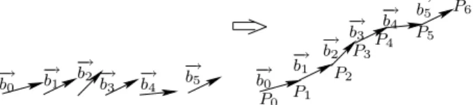
Let us consider the curve ζ1= {P }ni=0that is constructed by this rule:
−−−−→
PiPi+1=
− →
bi, i = 0, .., n − 1 (see Fig. 4).
Proposition 2. The estimation of tangent vector at each point Pi of the curve ζ1
− → b1 P0 P1 − → b4 − → b5 − → b5 P3 P4 P5 − → b0 − → b0 − → b1 − → b2−→ b3 − → b4 P2 P6 − → b2 − → b3
Fig. 4. The curve ζ1is constructed from the sequence of binormal vectors.
Proof. In differential geometry, the tangent vector of a curve r(t) at the point
Pt0 = r(t0) is defined as: t(t0) = r ′ (t0) = limh→0r(t0+h)−r(th 0) = limh→0 −−−→ Pt0P h .
Therefore, in discrete space, the tangent vector at the point Pi = α(i) can be
estimated as t(i) = r(i+1)−r(i)1 = −−−−→PiPi+1
1 = −−−−→ PiPi+1= − → bi.
Proposition 3. The torsion value at each point of the 3D discrete curve ζ
corre-sponds to the curvature value of the curve ζ1.
Proof. Thanks to definition 5.4, the discrete torsion at Ck of ζ curve is the
deriva-tive of−→bk. In addition,
− →
bk is the tangent vector at the kthpoint of ζ1curve. So,this
value is also curvature value at the kthpoint of ζ
1 curve.
Algorithm 4:Width ν torsion estimation at each point of ζ
Data: ζ 3D discrete curve of n points, ν width of the segmentation Result: {Tν(Ck)}k=0..n−1- Torsion of width ν at each point of ζ
begin Build M BSν= {M BSi(Bi, Ei, ν)}i=0 to m−1; m= |M BSν|; E−1= −1; Bm= n; fori= 0 to m − 1 do fork= Ei−1+ 1 to EidoL(k) = Bi; fork= Bi to Bi+1− 1 do R(k) = Ei; fori= 0 to n − 1 do − → t1 = −−−−−→ CiCL(I) |−−−−−→CiCL(i)| ;−→t2 = −−−−−→ CiCR(i) |−−−−−→CiCR(i)| ;−→bi =−→t1 ∧−→t2; Construct ζ1= {Pk}nk=0, with −−−−−→ PkPk+1=−→bk ;
Estimate the curvature value of width ν at each point of the curve ζ1as torsion
value of corresponding point of the curve ζ (see Algorithm 2); end
Remark: The bounds mentioned in the algorithm 4 are similar to the ones in the algorithm 3.
Therefore, by using these two propositions, we can estimate the torsion value at each point of ζ curve by determining the curvature value at the corresponding
points of curve ζ1. Our proposed method is presented in the algorithm 4, which
6. Experiments and comparisons 6.1. Experiments
We evaluated our methods on this computer configuration: CPU Pentium 4 with 3.2GHz, 1G of RAM, linux kernel 2.6.22-14 operating system. Because the estimated result is not correct for the beginning and the end of an open curve (see the bounds mentioned in the algorithms 2 and 3), during the phase of error estimation, we use a border parameter to eliminate this influence.
6.1.1. Error measure
We introduce three criteria for measuring error: mean relative error (meanRE), max relative error (maxRE) and quadratic relative error (QRE). Let us consider 2
sequences: the actual results {IRi}ni=1 and the estimated results {RRi}ni=1 at each
position. Then, we can define:
meanRE= 1 n n X i=1 |RRi− IRi| IRi (1) maxRE= max |RRi− IRi| IRi ff , i= 1, .., n (2) QRE= v u u t 1 n n X i=1 8 > : |RRi− IRi| IRi 9 > ; 2 (3)
These criteria are modified from clasic error criteria. They allow us to measure how an estimated result respects the profile of an actual result.
6.1.2. Curvature experiments
We present in Fig. 5 some experiments with our curvature estimator for planar curves. Two discrete curves (Fig. 5.a and 5.c) are presented with the plot of their curvature values calculated at each point of the curves with width 2 (Fig. 5.b and 5.d). The points of the curve 5.c that correspond to the peaks (black squares) of the associated curvature graph 5.d, are indicated by black pixels. We recognize that these black pixels are well located on the corners of the curve 5.c. As a result, an application for corner detection can be deduced based on this curvature estimator. For 3D curves, Fig. 6 presents some experiments with our 3D curvature estimator
on some actual spatial discrete curves: helix, Viviani’s curve,...a with their actual
curvature profiles (Fig. 6.b and 6.e) and their estimated curvature profiles using by our estimator (Fig. 6.c and 6.f).
Concerning the error approximation, the Tab. 1 shows the error of our method in relation with actual results when we test with these above curves.
6.1.3. Torsion experiments
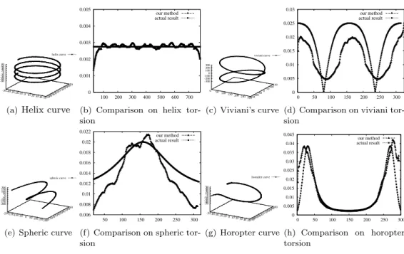
We present some experiments of our method on some ideal 3D curves : helix, Vi-viani’s, spheric, horopter and hyper helix curves. The tests are done after a process of discretisation of these 3D curves (see Fig. 7).
(a) Noisy circle, radius = 20 -0.08 -0.07 -0.06 -0.05 -0.04 -0.03 -0.02 -0.01 0 10 20 30 40 50 60 70 80 90 actual result our result
(b) max=-0.0444, min=-0.0531, mean=-0.0474 (c) -0.25 -0.2 -0.15 -0.1 -0.05 0 0.05 0.1 0.15 0.2 0 50 100 150 200 250 300 rabbit’s curvature (d) max=0.1761, min=-0.201
Fig. 5. Examples of 2D curvature extraction with ν = 2: (a) A discrete circle (radius=20) - (b) associated curvature profile. (c) A rabbit discrete curve - (d) associated curvature profile.
Curves N0
Border meanRE maxRE QRE Time
Circle 90 6 0.0186 0.1118 0.0316 100
Helix 760 20 0.0074 0.0519 0.0132 610
Viviani 274 20 0.1185 0.7248 0.2198 200
Table 1. Error estimation on the curvature results, N0: number of points, time is caculated in ms.
In most cases presented in Tab. 2 and Fig. 7, the mean relative errors do not overtake 0.15, and the quadratic relative errors do not overtake 0.015. If the actual torsion of the input curve has a value which is close to 0 at some positions, the obtained result is not very good. Let’s see the case of Viviani’s curve in the Tab. 2 (without threshold) and Fig. 9.a. In this case, the maximal relative error is high (15.6036). In spite of that, the mean relative error is acceptable (0.628899). In particular cases, if most of input curves has a torsion value which is close to 0, the obtained result is the worst (see Fig. 8, Fig. 9.b).
Like other approximation methods, our method doesn’t perform well when the actual value of the torsion approximates zero. It comes from the formula of relatif error. The divergence between actual value and estimated value reduce slowly when the actual value is close to 0. So the relatif error is so high in this situation. Let
-50-40-30-20-10 0 10 20 30 40 50-50-40-30-20 -10 0 10 20 30 40 50 -80 -60 -40 -20 0 20 40 60 80 helix curve
(a) Helix curve
0.014 0.016 0.018 0.02 0.022 0.024 0.026 0.028 100 200 300 400 500 600 700 actual result our result
(b) Comparison on helix curvature
0 50 100 150 200 250 300-150-100 -50 0 50 100 150 -300 -200 -100 0 100 200 300 viviani curve (c) Viviani curve 0 0.0005 0.001 0.0015 0.002 0.0025 0.003 0.0035 0.004 0.0045 0 50 100 150 200 250 300 our result actual result
(d) Comparison on viviani curvature Fig. 6.Experiments of curvature estimator, working width ν = 2
Curves N0 N1 meanRE maxRE QRE
Time
Without With Without With Without With
Spheric 255 30 0.1317 0.1317 0.3428 0.3428 0.1642 0.1642 280
Horopter 239 30 0.0827 0.0827 0.1862 0.1862 0.0979 0.0979 300
Helix 760 30 0.0481 0.0481 0.5145 0.5145 0.0814 0.0814 920
Viviani 274 30 0.6289 0.4570 15.6036 3.5128 1.6228 0.6156 290
Hyperhelix 740 30 8551.24 1.1527 154378 3.8019 24704.2 1.6210 720
Table 2. Error estimation on the torsion results without (with a threshold), N0: number of points, N1: border, time is caculated in ms. In the second line, without: without threshold; with: with a threshold = 0.0005
Estimator N0 N1 meanRE maxRE QRE Time
Without With Without With Without With
Curvature 274 30 0.5191 0.5010 1.0618 1.0085 0.7355 0.7098 NA
Torsion 274 30 0.5367 0.4987 1.2160 1.0036 0.7615 0.7066 NA
Table 3. Error estimation on the curvature and torsion results of Lewiner’s method on viviani’s curve without (with a threshold), N0: number of points, N1: border, time is caculated in ms. In the second line, without: without threshold; with: with a threshold = 0.0005
us consider the case of an hyper helix curve (see Fig. 8). The problem is that the torsion approximation is not good at nearly-0 values. In spite of that, the
-50-40-30-20-10 0 10 20 30 40 50-50-40-30-20-10 0 10 20 30 40 50 -80 -60 -40 -20 0 20 40 60 80 helix curve
(a)Helix curve
0 0.001 0.002 0.003 0.004 0.005 100 200 300 400 500 600 700 our method actual result
(b) Comparison on helix tor-sion 0 50 100 150 200 250 300-150-100 -50 0 50 100 150 -300 -200 -100 0 100 200 300 viviani curve (c) Viviani’s curve 0 0.005 0.01 0.015 0.02 0.025 0.03 0 50 100 150 200 250 300 our method actual result
(d) Comparison on viviani tor-sion -200-150-100 -50 0 50 100 150 200 0 10 20 30 40 50 60 70 80 90 -200 -150 -100-50 0 50 100 150 200 spheric curve
(e) Spheric curve
0.006 0.008 0.01 0.012 0.014 0.016 0.018 0.02 0.022 50 100 150 200 250 300 our method actual result
(f) Comparison on spheric tor-sion -50-40-30-20-10 0 10 20 30 40 50-100-80-60-40-20 0 20 40 60 80 100 -50 -40 -30 -20 -10 10 0 20 30 40 50 horopter curve (g) Horopter curve 0 0.005 0.01 0.015 0.02 0.025 0.03 0.035 0.04 0.045 0 50 100 150 200 250 300 our method actual result (h) Comparison on horopter torsion
Fig. 7.Experiments on torsion estimator, working width ν= 2.
0 500000 1e+06 1.5e+06 2e+06 2.5e+06
3e+06 3.5e+06-4e+06-3e+06-2e+06 -1e+06 0
1e+06 2e+06 3e+06 4e+06 -3000 -2000 -1000 0 1000 2000 3000 hyperhelix curve
(a) Hyperhelix curve
0 0.002 0.004 0.006 0.008 0.01 0.012 0.014 0.016 0.018 0 100 200 300 400 500 600 700 800 our method actual result
(b) Comparison on hyperhelix tor-sion
Fig. 8.Most of the hyper helix curve has a torsion value close to 0. So in this case, the obtained result is the worst.
approximation value is also close to 0 but the relative rate between approximation value and actual value is very high. In the Fig. 9.b, we show the relation between approximation torsion and actual torsion of an hyper helix curve from the index 15 and to the index 250. In this index interval, the actual torsion is close to 0. So, the relative error between approximation torsion and actual torsion is very high, in spite of that the approximation value does not overtake 0.006. So, we propose to consider only the points whose actual torsion value is greater than the threshold. In the equations 1, 2 and 3, n is replaced by number of points whose actual torsion value is greater than a threshold. The Tab. 2 shows also the approximated error
0 0.005 0.01 0.015 0.02 0.025 0.03 0 50 100 150 200 250 300 350 actual result of viviani’s curve
(a) 0 0.0002 0.0004 0.0006 0.0008 0.001 0.0012 0.0014 50 100 150 200 250 actual result our result (b)
Fig. 9. a:Torsion of Viviani’s curve; b:The actual torsion and our result obtained with a hyperhelix curve between the index 15 and 250.
Curves No Border Sigma meanRE maxRE QRE Time
Hyper helix 740 30 4 0.451744 5.39524 0.796259 200 Spheric 255 30 9 0.32234 0.852819 0.47207 140 - − − 10 0.315752 0.843035 0.461791 220 - − − 12 0.302302 0.962883 0.442564 290 Viviani 274 30 7 0.466501 0.999349 0.664052 100 - − − 9 0.457997 0.996809 0.653339 140 - − − 12 0.451581 0.994291 0.643084 300
Table 4. Error estimation on the torsion results with Mokhtarian’s method, No: number of points, time is caculated in ms. Implementation is developped and run on Matlab 7.5.0.
with a threshold equal to 0.0005.
6.2. Comparisons to other approachs
We compare our estimators to some well-known methods in the literature.
Mokhtarian’s approach: Mokhtarian 24,7 proposed an approach using a scale
space technique which is based on Gaussian fitting.
A planar curve, Γ is first parameterized by the arc length parameter u: Γ =
(x(u), y(u)). By using Gaussian fitting, an evolved version Γσ is computed: Γσ =
(X(u, σ), Y (u, σ)) = (x(u) ⊗ g(u, σ), y(u) ⊗ g(u, σ)), where g(u, σ) = 1
σ√2πe
−u2 2σ2 So
the curvature at each point can be computed on the evolved curve Γσ as follows
κ(u, σ) =Xu(u, σ)Yuu(u, σ) − Xuu(u, σ)Yu(u, σ) p(Xu(u, σ)2+ Yu(u, σ)2)3
where Xu(u, σ) = x(u) ⊗ gu(u, σ), Xuu(u, σ) = x(u) ⊗ guu(u, σ), Yu(u, σ) =
y(u)⊗gu(u, σ), Yuu(u, σ) = y(u)⊗guu(u, σ), gu(u, σ) =∂g(u,σ)∂u , guu(u, σ) =∂∂g(u,σ)∂∂u
Similarly, in the case of spatial curve, an evolved version of the curve is Γσ =
(X(u, σ), Y (u, σ), Z(u, σ)). So, the curvature and torsion can be calculated respec-tively as follows.
κ(u, σ) =p(XuYuu− XuuYu)2+ (YuZuu− YuuZu)2+ (ZuXuu− ZuuXu)2 p(X2
τ(u, σ) =Xu(YuuZuuu− ZuuYuuu) + Yu(ZuuXuuu− XuuZuuu) + Zu(XuuYuuu− YuuXuuu) (XuYuu− XuuYu)2+ (YuZuu− YuuZu)2+ (ZuXuu− ZuuXu)2
Lewiner et al’s approach: Lewiner et al. 5,25 proposed curvature and torsion
estimators based on a parametric curve fitting technique that uses weighted
least-squares fitting. Consider a sequence of points {pi} on a smooth curve r. For each
point pj, he considered a window of 2q + 1 points around pj = r(j) to estimate the
derivatives of r(s). Let si be the arc-length corresponding to sample pi. It can be
estimated as li =
i−1
X
k=0
pkpk+1. To determine curvature, considering that p0 = r(0)
is the origin, he used the second order approximation: r(s) = r′(0)s +1
2r
′′
(0)s2+
g1(s)s3with lim
s→0g1(s) = 0. The estimation of derivatives are obtained by a weighted
least square minimization. Consider the case of a planar curve. His idea is to locally
fit a parametric curve (ˆx(s), ˆy(s)) to the curve, with one of the coordinate functions,
say ˆx, being quadratic in the arc-length: ˆx(s) = x0+ x
′
0.s+12x
′′
0.s2. The derivatives
x′0and x′′0 can be estimated by minimizingEx(x′0, x
′′ 0) = q X i=−q ωi(xi− x ′ 0li− 1 2x ′′ 0(li)2)2.
The weight ωi of the point pi can be considered simply ωi = 1. The estimates y
′
0
and y0′′ are obtained by both the unit norm of the tangent and the orthogonality
of the tangent and the normal: (x′
0)2+ (y ′ 0)2= 1 and x ′ 0x ′′ 0 + y ′ 0y ′′ 0 = 0. A similar
approach with spatila curve. So the curvature can be calculated by this formula:
κ(t, q, σ) = r
′
× r′′ ||r′′′||
For torsion estimation, the third order approximation is used: r(s) = r′(0)s +
1 2r ′′ (0)s2+1 6r ′′′ (0)s3+ g2(s)s4 i+ with lim
s→0g2(s) = 0. For spatial curve, the torsion
estimator fits a cubic parametric curve to the sample points. So, x′
0, x ′′ 0 and x ′′′ 0 should minimize: Ex(x′0, x ′′ 0), x ′′′ 0 = q X i=−q ωi(xi− (x ′ 0si+ 1 2x ′′ 0s 2 i + 1 6x ′′′ 0 s 3 i)) 2. A similar
approach is used to computed y0′, y
′′ 0, y ′′′ 0, z ′ 0, z ′ 0, z ′′′
0 . The torsion is given by
τ(t, q, σ) =(r
′
× r′′).r′′′ ||r′× r′′||2
Comparison: We present in Fig. 10, 11 and Tab. 3, 4 a comparison between our estimators and these methods. We admit that the result of Mokhtarian’s method depends largely on the value of the parameter σ. When the value of σ is too small, the obtained result is very noisy, but the higher value for σ can lead to inexact results and margin effects in which the result is totally different from actual result. Our method use 1 parameter that is the width, Mokhtarian’s method used 1 parameter that is σ. Lewiner’s method use 2 different parameters (σ and q), so the number of parameters of this method is more than 2 others. The result of this torsion estimator seems to be more noisy than other methods. Concerning the quality of approximated results, our method is better than 2 methods, but among these 3 methods, the method of Mokhtarian is the fastest thanks to its linear complexity.
0 0.002 0.004 0.006 0.008 0.01 0 50 100 150 200 250 our result actual result Lewiner’s result
(a) Comparison on curvature estimator 0 0.005 0.01 0.015 0.02 0.025 0.03 0 50 100 150 200 250 actual result our result Lewiner’s result
(b) Comparison on torsion estimator Fig. 10. Comparisons between our curvature and torsion estimators with Lewiner’s approach on Viviani’s curve. The results of Lewiner are supplied by the author.
7. Conclusions
We have presented in this paper the methods to estimate curvature for planar curves, and the curvature and torsion for spatial curves. These methods benefit
from the improvement of curvature estimator in 2D case 3, so they are efficient
than using existent method1,17 for blurred segment recognition to construct these
estimators.
These estimators permit to extract local properties of spatial curves. We hope to identify and classify 3D objects by using these estimators. Our work can also be applied for an application to fibres in 3D images of paper that has been presented
in 13. Another applications can be geometric compression 25 or medical imaging
9. In the futur, we will look for an application for DNA curve matching based on
curvature and torsion estimation. Acknowledgements
A preliminary version of this work was presented at the International Symposium on Visual Computing, Las Vegas, NV, 2008, Special Track on Discrete and
Com-putational Geometry and their Applications in Visual Computing26.
We would like to thank Thomas Lewiner for supplying his program to evaluate performance.
We would like to thank the reviewers for their constructive and detailed com-ments that permit us to improve the manuscript.
References
1. I. Debled-Rennesson, F. Feschet, J. Rouyer-Degli, Optimal blurred segments decom-position of noisy shapes in linear time, Computers & Graphics 30 (1).
2. J.-P. Reveill`es, G´eom´etrie discr`ete, calculs en nombre entiers et algorithmique, th`ese d’´etat. Universit´e Louis Pasteur, Strasbourg (1991).
3. T. P. Nguyen, I. Debled-Rennesson, Curvature estimation in noisy curves, in: CAIP, Vol. 4673 of Lecture Notes in Computer Science, Springer, 2007, pp. 474–481. 4. J.-P. Salmon, I. Debled-Rennesson, L. Wendling, A new method to detect arcs and
-0.2 -0.15 -0.1 -0.05 0 0.05 0.1 0 20 40 60 80 100 120 Our method,width=2 Mokhtarian’s method, sigma=6 Mokhtarian’s method, sigma=3
(a) -0.2 -0.15 -0.1 -0.05 0 0.05 0.1 0 50 100 150 200 250 300 350 400
Our method, width=3 Mokhtarian’s method, sigma=9
(b) 0 0.05 0.1 0.15 0.2 0.25 0.3 0 50 100 150 200 250 300 350 400
Our method, width=3 Mokhtarian’s method, sigma=9
(c)
Fig. 11. a. Comparison between our 2D curvature estimator and Mokhtarian’s 2D curvature esti-mator on a circle, radius is 20; b (resp. c): Comparison between our 3D curvature (resp. torsion) estimators and Mokhtarian’s 3D curvature (resp. torsion) estimators on an helix curve.
5. T. Lewiner, J. D. G. Jr., H. Lopes, M. Craizer, Curvature and torsion estimators based on parametric curve fitting., Computers & Graphics 29 (5) (2005) 641–655. 6. E. Attneave, Some informational aspects of visual perception, Psychol. Rev. 61 (3). 7. F. Mokhtarian, A theory of multiscale, torsion-based shape representation for space
curves., Computer Vision and Image Understanding 68 (1) (1997) 1–17.
8. N. D. Kehtarnavaz, R. J. P. de Figueiredo, A 3-d contour segmentation scheme based on curvature and torsion, IEEE Trans. Pattern Anal. Mach. Intell. 10 (5) (1988) 707–713.
9. R. Medina, A. Wahle, M. E. Olszewski, M. Sonka, Curvature and torsion estimation for coronary-artery motion analysis, in: SPIE Medical Imaging, Vol. 5369, 2004, pp. 504–515.
10. F. Feschet, L. Tougne, Optimal time computation of the tangent of a discrete curve: Application to the curvature., in: DGCI, Vol. 1568 of LNCS, 1999, pp. 31–40. 11. D. Coeurjolly, S. Miguet, L. Tougne, Discrete curvature based on osculating circle
12. J.-O. Lachaud, A. Vialard, F. de Vieilleville, Analysis and comparative evaluation of discrete tangent estimators., in: DGCI, Vol. 3429 of LNCS, 2005, pp. 240–251. 13. D. Coeurjolly, S. Svensson, Estimation of curvature along curves with application to
fibres in 3d images of paper, in: SCIA, 2003, pp. 247–254.
14. I. Debled-Rennesson, Reconnaissance des droites et plans discrets, Ph.D. thesis, Louis Pasteur University (1995).
15. D. Coeurjolly, I. Debled-Rennesson, O. Teytaud, Segmentation and length estimation of 3d discrete curves, in: Digital and Image Geometry, Vol. 2243 of LNCS, Springer, 2000, pp. 299–317.
16. M. Overmars, J. van Leeuwen, Maintenance of configurations in the plane, J. Comput. and Syst. Sci. 23 (1981) 166–204.
17. L. Buzer, An elementary algorithm for digital line recognition in the general case., in: DGCI, Vol. 3429 of LNCS, 2005, pp. 299–310.
18. A. V. Aho, J. E. Hopcroft, J. D. Ullman, The Design and Analysis of Computer Algorithms, Addison-Wesley, Reading, Mass., 1974.
19. I. Debled-Rennesson, Estimation of tangents to a noisy discrete curve, in: Vision Geometry XII, SPIE, Vol. 5300, 2004, pp. 117–126.
20. A. Rosenfeld, E. Johnston., Angle detection on digital curves, IEEE Transactions on Computers (1973) 875–878.
21. J. Harris, H. Stocker, Handbook of mathematics and computational science, Springer-Verlag, 1998.
22. J. Oprea, Differential geometry and its applications, 2007.
23. M. Worring, A. W. M. Smeulders, Digital curvature estimation., Computer Vision Graphics Image Processing: CVIU 58 (3) (1993) 366–382.
24. F. Mokhtarian, A. K. Mackworth, A theory of multiscale, curvature-based shape rep-resentation for planar curves, IEEE Trans. Pattern Anal. Mach. Intell. 14 (8) (1992) 789–805.
25. T. Lewiner, J. D. G. Jr., H. Lopes, M. Craizer, Arc-length based curvature estimator, in: SIBGRAPI, 2004, pp. 250–257.
26. T. P. Nguyen, I. Debled-Rennesson, Curvature and torsion estimators for 3d curves, in: ISVC (1), Vol. 5358 of Lecture Notes in Computer Science, Springer, 2008, pp. 688–699.