Closure Schemes for Nonlinear Bistable Systems
Subjected to Correlated Noise: Applications
to Energy Harvesting from Water Waves
The MIT Faculty has made this article openly available.
Please share
how this access benefits you. Your story matters.
Citation
Joo, Han Kyul, and Themistoklis Sapsis. “Closure Schemes for
Nonlinear Bistable Systems Subjected to Correlated Noise:
Applications to Energy Harvesting from Water Waves.” Journal of
Ocean and Wind Energy 2, no. 2 (May 2015).
As Published
http://dx.doi.org/10.17736/jowe.2015.mmr10
Publisher
International Society of Offshore and Polar Engineers
Version
Author's final manuscript
Citable link
http://hdl.handle.net/1721.1/109333
Terms of Use
Creative Commons Attribution-Noncommercial-Share Alike
Closure Schemes for Nonlinear Bi-stable Systems subjected to Correlated Noise
- Applications to Energy Harvesting from Water Waves
Han Kyul Joo and Themistoklis P. Sapsis
Department of Mechanical Engineering, Massachusetts Institute of Technology Cambridge, Massachusetts, USA
ABSTRACT
Moment Equation Closure Minimization (MECM) method has been developed for the inexpensive approximation of the steady state statistical structure of bistable systems which have bimodal potential shapes and which are subjected to correlated excitation. Our approach relies on the derivation of moment equations that describe the dynamics governing the two-time statistics. These are then combined with a closure scheme which arises from a non-Gaussian pdf representation for the joint response-excitation statistics. We demonstrate its effectiveness through the application on a bistable nonlinear single-degree-of-freedom ocean wave energy harvester with linear damping and the results compare favorably with direct Monte Carlo Simulations. KEY WORDS: Moment Equations, Non-Gaussian Closure, Two-time Response Statistics, Ocean Wave Energy Harvester, Bistable System, Colored Noise Excitation, Nonlinear Dynamics.
INTRODUCTION
In numerous systems in engineering, uncertainty in the dynamics is as important as the known conservation laws. Such an uncertainty can be introduced due to external stochastic excitations, e.g. energy harvesters or structural systems subjected to ocean waves, wind excitations, earthquakes, and impact loads (Grigoriu, 2002; Stratonovich, 1967; Sobczyk, 2001; Soong and Grigoriu, 1993; Naess and Moan, 2012; To, 2011). For these cases deterministic models cannot capture or even describe the essential features of the response and to this end, understanding of the system dynamics and optimization of its parameters for the desired performance is a challenging task. On the other hand a probabilistic perspective can, in principle, provide with such information but then the challenge is the numerical treatment of the resulting descriptive equations, which can be associated with prohibitive computational cost.
The focal point of this work is the development of computational methods for the inexpensive probabilistic description of nonlinear vibrational systems of low to moderate dimensionality subjected to correlated excitations. Depending on the system dimensionality and its dynamical characteristics, numerous techniques have been developed to
quantify the response statistics, i.e. the probability density function (pdf) for the system state. For systems subjected to white noise, Fokker-Planck equation provides with a complete statistical description of the response statistics (Wojtkiewicz et al., 1999; Dunne and Ghanbari, 1997; Di Paola and Sofi, 2002). On the other hand, for systems subjected to correlated excitations the joint response-excitation method provides with a computational framework for the full statistical solution (Sapsis and Athanassoulis, 2008; Venturi et al., 2012; Cho et al, 2013). However, such methodologies rely on the solution of transport equations for the pdf and they are associated with very high computational cost especially when it comes to the optimization of system parameters.
To avoid the solution of transport equations for the pdf, semi-analytical approximative approaches have been developed that reduce significantly the computational cost. Among them the most popular in the context of structural systems is the statistical linearization method (Caughey, 1959; Caughey, 1963; Kazakov, 1954; Roberts and Spanos, 2003; Socha, 2008), which can also handle correlated excitations. The basic concept of this approach is to replace the original nonlinear equation of motion with a linear equation, which can be treated analytically, by minimizing the statistical difference between those two equations. Statistical linearization performs very well for systems with unimodal statistics, i.e. close to Gaussian. However, when the response is essentially nonlinear e.g. as it is the case for a double-well oscillator, the application of statistical linearization is less straightforward and involves the ad-hoc selection of shape parameters for the response statistics (Crandall et al., 2005).
An alternative class of methods relies on the derivation of moment equations, describing the evolution of the the joint response-excitation statistical moments or (depending on the nature of the stochastic excitation) the response statistical moments (Sancho, 1970; Bover, 1978; Beran, 1994). The challenge with moment equations arises if the system equation contains nonlinear terms in which case we have the well-known closure problem. This requires the adoption of closure schemes or methods, which essentially truncate the infinite system of moment equations to a finite one. The simplest approach along these lines is the Gaussian closure (Iyengar and Dash, 1978) but nonlinear closure schemes have also been developed (Crandall, 1980; Crandall, 1985; Liu and Davies, 1988; Wu and Lin, 1984; Ibrahim, 1985;
Grigoriu, 1991; Hasofer and Grigoriu, 1995; Wojtkiewicz et al., 1996; Grigoriu, 1999). In most cases these nonlinear approaches may offer some improvement compared with the stochastic linearization approach applied to nonlinear systems but the associated computational cost is considerably larger (Noori et al., 1987). For strongly nonlinear systems, such as bistable systems, these improvements can be very small. The latter have become very popular in energy harvesting applications (Green et al., 2012; Harne and Wang, 2013; Daqaq, 2011; Halvorsen, 2013; Green et al., 2013; He and Daqaq, 2014; Mann and Sims, 2009; Barton et al., 2010), where there is a need for fast and reliable calculations that will be able to resolve the underlying nonlinear dynamics in order to provide with optimal parameters of operation (Joo and Sapsis, 2014; Kluger et al., 2015).
The goal of this work is the development of a closure methodology that can overcome the limitations of traditional closure schemes and can approximate the steady state statistical structure of bistable systems excited by correlated noise. We first formulate the moment equations for the joint pdf of the response and the excitation at two arbitrary time instants (Athanassoulis et al., 2013). To close the resulting system of moment equations we formulate a two-time representation of the joint response-excitation pdf. We chose the representation so that the single time statistics are consistent in form with the Fokker-Planck solution in steady state, while the correlation between two different time instants is assumed to have a Gaussian structure. Based on these two ingredients (dynamical information expressed as moment equations and assumed form of the response statistics) we formulate a minimization problem with respect to the unknown parameters of the pdf representation so that both the moment equations and the closure induced by the representation are optimally satisfied. For the case of unimodal systems the described approach reproduces the statistical linearization method while for bi-modal systems it still provides with meaningful and accurate results with very low computational cost.
The developed approach allows for the inexpensive and accurate approximation of the second order statistics of the system even for oscillators associated with double-well potentials. In addition, it allows in a post-processing manner for the semi-analytical approximation of the full non-Gaussian joint response-excitation pdf. We illustrate the developed approach through a nonlinear single-degree-of-freedom ocean wave energy harvester with double-well potential subjected to correlated noise of Pierson-Moskowitz power spectral density. We demonstrated how the proposed probabilistic framework can be used for performance optimization and parameters selection.
METHOD DESCRIPTION
In this section, we give a detailed description of the proposed method for the inexpensive computation of the response statistics for dynamical systems subjected to colored noise excitation. The computational approach relies on two basic ingredients:
• Two time statistical moment equations. These equations will be derived directly from the system equation and they will express the dynamics that govern the two-time statistics. For systems excited by white-noise, single time statistics are sufficient to describe the response but for correlated excitation this is not the case and it is essential to consider higher order moments. Note that higher (than two) order statistical moment equations may be used but in the context of this work two-time statistics would be sufficient.
• Probability density function (pdf) representation for the joint response-excitation statistics. This will be a family of probability
density functions that will express geometrical properties of the solution such as multi-modality, tail decay properties, correlation structure between response and excitation, or others. In this work we will use representations inspired by the analytical solutions of the dynamical system when this is excited by white noise. These representations will reflect features of the Hamiltonian structure of the system and will be used to derive appropriate closure schemes that will be combined in the moment equations.
Based on these two ingredients we will formulate a minimization problem with respect to the unknown parameters of the pdf representation so that both the moment equations and the closure induced by the proposed representation are optimally satisfied. We will see that for the case of unimodal systems the described approach reproduces the statistical linearization method while for bi-modal systems it still provides with meaningful and accurate results with very low computational cost.
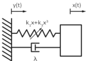
For the sake of simplicity we will present our method through a specific system involving a nonlinear SDOF oscillator with a double well potential. This system has been studied extensively in the context of energy harvesting especially for the case of white noise excitation (Daqaq, 2011; Daqaq, 2012; Gammaitoni et al., 2009; Ferrari et al., 2010). However, for realistic setups it is important to be able to optimize/predict its statistical properties under general (colored) excitation. More specifically we consider a nonlinear harvester of the form . = 3 3 1x kx y k x x!!+λ!+ + !! (1)
where x is the relative displacement between the harvester mass and the base, y is the base excitation representing a stationary stochastic process, λ is normalized (with respect to mass) damping coefficient, and k and 1 k3 are normalized stiffness coefficients.
Fig. 1: Nonlinear energy harvester with normalized system parameters. Two-time moment system
We consider two generic time instants, t and s . We multiply the equation of motion at time t with the response displacement x(s) and apply the mean value operator (ensemble average). This will give us an equation which contains an unknown term on the right hand side. To determine this term we repeat the same steps but we multiply the equation of motion with y(s). This gives us the following two-time moment equations: , ) ( ) ( = ) ( ) ( ) ( ) ( ) ( ) ( ) ( ) (tys xt ys k1xt ys k3xt3ys yt ys x!! +λ! + + !! (2) .) ( ) ( = ) ( ) ( ) ( ) ( ) ( ) ( ) ( ) (txs xtxs k1xtxs k3xt3xs ytxs x!! +λ! + + !! (3)
Here the excitation is assumed to be a stationary stochastic process with zero mean and a given power spectral density; this can have an arbitrary form, e.g. monochromatic, colored, or white noise. Since the
system is characterized by an odd restoring force, we expect that its response will also have zero mean. Moreover, we assume that after an initial transient the system will be reaching a statistical steady state given the stationary character of the excitation. Based on properties of mean square calculus (Sobczyk, 2001; Beran, 1994) we interchange the differentiation and the mean value operators. Then the moment equations will take the form:
, ) ( ) ( = ) ( ) ( ) ( ) ( ) ( ) ( ) ( ) ( 2 2 3 3 1 2 2 s y t y t s y t x k s y t x k s y t x t s y t x t ∂ ∂ + + ∂ ∂ + ∂ ∂ λ (4) .) ( ) ( = ) ( ) ( ) ( ) ( ) ( ) ( ) ( ) ( 3 22 3 1 2 2 s x t y t s x t x k s x t x k s x t x t s x t x t ∂ ∂ + + ∂ ∂ + ∂ ∂ λ (5)
Expressing everything in terms of the covariance functions will result in: , = ) ( ) ( 2 2 3 3 1 2 2 ts yy ts xy ts xy ts xy C t s y t x k C k C t C t ∂ ∂ + + ∂ ∂ + ∂ ∂ λ (6) , = ) ( ) ( 2 2 3 3 1 2 2 ts yx ts xx ts xx ts xx C t s x t x k C k C t C t ∂ ∂ + + ∂ ∂ + ∂ ∂ λ (7)
where the covariance function is defined as
.) ( = ) ( = ) ( ) ( = xy xyτ ts xy xtys C t s C C − (8)
Taking into account the assumption for a stationary response (after the system has gone through an initial transient phase) the above moment equations can be rewritten in terms of the time difference τ=t −s:
), ( = ) ( ) ( ) ( ) ( ) ( 2 2 3 3 1 2 2 τ τ τ τ τ λ τ τ Cxy Cxy kCxy k xt ys ∂ Cyy ∂ + + ∂ ∂ + ∂ ∂ (9) ). ( = ) ( ) ( ) ( ) ( ) ( 2 2 3 3 1 2 2 τ τ τ τ τ λ τ τ ∂ − ∂ + + ∂ ∂ + ∂ ∂ xy xx xx xx C kC k xt xs C C (10)
The above procedure completes the derivation of the moment equations describing the dynamics of the system in statistical steady state. Note that all the linear terms in the original system's equation are expressed in terms of the covariance functions, while the nonlinear (cubic) terms show up in the form of fourth order moments. To compute the latter we will need to adopt an appropriate closure scheme.
Two-time PDF Representation and induced closure schemes In the absence of higher-than-two order moments, the response statistics can be analytically obtained in a straightforward manner. However, for higher order terms it is necessary to adopt an appropriate closure scheme that will close the infinite system of moment equations. A standard approach in this case, which performs very well for unimodal systems, is the application of Gaussian closure which utilizes Isserlis’ Theorem (Isserlis, 1918) to connect the higher order moments with the second order statistical quantities. Despite its success for unimodal systems, Gaussian closure does not provide accurate results for bistable systems. This is because in this case the closure induced by the Gaussian assumption does not reflect the properties of the system attractor in the statistical steady state.
Here we aim to solve this problem by proposing a non-Gaussian representation for the joint response-response pdf at two different time instants and for the joint response-excitation pdf at two different time instants. These representations will:
• incorporate specific properties or information about the response
pdf (single time statistics) in the statistical steady state,
• incorporate a given correlation structure between the statistics of the response and the excitation, e.g. Gaussian,
• have a consistent marginal with the excitation pdf (for the case of the joint response-excitation pdf),
• induce a non-Gaussian closure scheme that will be consistent with all the above properties.
1) Representation properties for single time statistics.
We begin by introducing the pdf properties for the single time statistics. The selected representation will be based on the analytical solutions of the Fokker-Planck equation which are available for the case of white noise excitation (Soize, 1994; Sobczyk, 2001), and for vibrational systems that has an underlying Hamiltonian structure. Here we will leave the energy level of the system as a free parameter - this will be determined later. In particular we will consider the following family of pdf solutions (Fig. 2a):
)}, 4 1 2 1 ( 1 { exp 1 = )} ( 1 { exp 1 = ) ; ( 4 3 2 1x kx k x U x f − − + γ γ γ F F (11)
where, U is the potential energy of the oscillator, γ is a free parameter connected with the energy level of the system, and F is the normalization constant expressed as follows:
. )} 4 1 2 1 ( 1 { exp =
∫
− k1x2+ k3x4 dx ∞ ∞ − γ F (12)Fig. 2: (a) Representation of the steady state pdf for single time statistics of a system with double-well potential. The pdf is shown for different values of the system’s energy level. (b) The joint response excitation pdf is also shown for different values of the correlation parameter c ranging from small values (corresponding to large values of |τ|) to larger ones (associated with smaller values of |τ|).
2) Correlation structure between two-time statistics.
Representing the single time statistics is not sufficient since for correlated excitation the system dynamics can be effectively expressed only through (at least) two-time statistics. Although the response steady state pdf is assumed to have a non-Gaussian form, we represent the correlation between two different time instants having a Gaussian structure. Based on this assumption we obtain pdf representations for the joint response-response and response-excitation at different time instants.
Joint response-excitation pdf. We first formulate the joint response-excitation pdf at two different time instants. Denoting with x the argument that corresponds to the response at time t , with y the argument for the excitation at time s =t−τ, and with g( y) the (zero-mean) marginal pdf for the excitation, we have the expression for the
joint response-excitation pdf , ) ( ) ( 1 = ) , (xy f xg yecxy q M (13)
where M indicates a normalization constant and c defines the degree of correlation between the response and the excitation.
We note that the semi-positive definite property of the covariance matrix, associated with this process, defines a range of possible values for the constant c . In particular, denoting with Σ the covariance matrix which describes the correlation at different time instants we have . = 2 2 ⎥ ⎥ ⎦ ⎤ ⎢ ⎢ ⎣ ⎡ Σ y xy xy x σ σ σ σ (14)
This matrix should be semi-positive definite, i.e. for every non-zero column vector u the following should be satisfied
0. ≥ Σu
uT (15)
Since the above matrix has a positive trace the semi-positive definite property is guaranteed if and only if the determinant is greater or equal to zero. This condition provides a relation between the covariance
σ
xy (connected with c ) and the variances of the marginal distributions:. 2 2 2 2 y x xy y xσ σ σ σ σ ≤ ≤ − (16)
To connect the covariance
σ
xy with c , we expand the former in a Taylor series keeping up to the third order terms in c :σxy= 1 M
∫∫
xyf (x)g(y)e cxydxdy = x2y2c +1 6{x 4y4− 3(x2)2(y2)2}c3. (17)This will give us the following condition for c
− x2y2 ≤ x2y2c +1 6{x 4y4 − 3(x2)2(y2)2}c3 ≤ x2y2. (18) For the systems considered in this paper we found that a third order expansion is necessary and sufficient for good numerical results.
Joint response-response pdf. The joint pdf for two different time instants of the response, denoted as p( zx, ) is a special case of what has been presented previously. In order to avoid confusion, a different notation z is used to represent the response displacement at a different time instant s . Then we have:
, ) ( ) ( 1 = ) , (xz f x f zecxz p N (19)
where N is a normalization constant and c is a correlation constant. As stated previously, the correlation between two time instants has been assumed to have a Gaussian structure and similar constraints on the possible values of c hold for this case as previously. We also note that the response displacement z at a different time instant still follows the same non-Gaussian pdf corresponding to the single time statistics of the response (Eq. 11).
In Fig. 2b, we present the above joint pdf (Eq. 13) with the marginal
f (response) having a bimodal structure and the marginal g (excitation) having a Gaussian structure. For c=0 we have independence, which essentially expresses the case of very distant two-time statistics, while as we increase c the correlation between the two variables increases referring to the case of small values of τ .
3) Induced non-Gaussian closure.
Fig. 3: The relation between x(t)3x(s) and x(t)x(s). Exact relation is illustrated in red curve and approximated relation using non-Gaussian pdf representations is depicted in black curve.
Using these non-Gaussian pdf representations we will approximate the fourth order moment terms that show up in the moment equations. In the context of the pdf representations given above, the relation between
) ( ) (t 3xs
x and x(t)x(s) is very close to linear (see Fig. 3). To this end we choose a closure of the form (for both the response-response and the response-excitation terms): , ) ( ) ( = ) ( ) (t3xs , xtxs x ρxx (20)
where
ρ
x,x is the closure coefficient. The value ofρ
x,x can be found if we expand both x(t)3x(s) and x(t)x(s) with respect to c . A first order Taylor expansion will giveρx,x= x4 x2 c x2 x2 c= x4 x2. (21)
Therefore, for a given marginal f we can find analytically what would be the closure coefficient under the assumptions of the adopted closure scheme. Note that this constant depends directly on the energy level of the system defined by γ since the moments x and 2 x4 depend on it. Similar relations can be derived for the term x(t)3y(s). We will refer to Eq. (21) as the closure constraint. This will be one of two constraints that we will include in the minimization procedure for the determination of the solution.
4) Closed Moment Equations.
The next step involves the application of the closure scheme above on the derived two-time moment equations. By direct application of the induced closure schemes on Eqs. (9) and (10), we have the linear set of moment equations for the second-order statistics:
), ( = ) ( ) ( ) ( ) ( 2 2 3 , 1 2 2 τ τ τ ρ τ τ λ τ τ Cxy Cxy k xyk Cxy ∂ Cyy ∂ + + ∂ ∂ + ∂ ∂ (22) ). ( = ) ( ) ( ) ( ) ( 2 2 3 , 1 2 2 τ τ τ ρ τ τ λ τ τ ∂ − ∂ + + ∂ ∂ + ∂ ∂ xy xx x x xx xx C k k C C C (23)
Using the Wiener-Khinchin theorem, we transform the above equations to the corresponding equations for the power spectral density:
), ( ) ( = ) ( } ) ( ) {(jω2+λ jω +k1+ρx,yk3Sxyω jω2Syyω (24) ). ( ) ( = ) ( } ) ( ) {(jω2−λ jω +k1+ρx,xk3 Sxxω jω2Sxy ω (25)
These equations allow us to obtain an expression for the power spectral density of the response displacement in terms of the excitation spectrum: ). ( | )} ( )}{ ( { =| ) ( 2 3 , 1 2 3 , 1 4 ω λω ω ρ λω ω ρ ω ω yy x x y x xx S j k k j k k S − − + + − + (26)
Integrating the last equation will give us the variance of the response displacement: . ) ( | )} ( )}{ ( { | = ) ( = 2 3 , 1 2 3 , 1 4 0 0 2 ω ω λω ω ρ λω ω ρ ω ω ω S d j k k j k k d S x yy x x y x xx − − + + − +
∫
∫
∞ ∞ (27)Minimizing the deviation of the right-hand-side from the left-hand-side of the last equation is the second constraint, the dynamics constraint, which we will try to minimize together with the closure constraint defined by Eq. (21). It expresses the second order dynamics of the system.
5) Moment Equation Closure Minimization (MECM) Method.
The last step is the minimization of the two constraints, the closure constraint (Eq. 21) and the dynamics constraint (Eq. 27), which have been expressed in terms of the system response variance x . The 2 minimization will be done in terms of the unknown energy level γ and the closure coefficient
ρ
x,x. More specifically, we define the following cost functional which incorporates the two constraints:. | )} ( )}{ ( { ) ( | = ) , ( 2 , 4 2 2 2 3 , 1 2 3 , 1 4 0 2 , ⎟⎟ ⎟ ⎠ ⎞ ⎜⎜ ⎜ ⎝ ⎛ − + ⎟ ⎟ ⎠ ⎞ ⎜ ⎜ ⎝ ⎛ − − + + − + −
∫
∞ x x x x y x yy x x d x x j k k j k k S x ρ ω λω ω ρ λω ω ρ ω ω ρ γ J (28)Note that in the context of statistical linearization only the first constraint is minimized while the closure coefficient is the one that follows exactly from a Gaussian representation. Therefore, in this context there is no attempt to incorporate in an equal way the effect of error in the dynamics and the error in the pdf representation. Minimization of this functional essentially imposes an interplay between these two factors in order to obtain a solution that satisfies both as close as possible. For linear systems and an adopted Gaussian pdf for the response, as expected, the above cost function vanishes identically.
We also emphasize that in the above cost function we have only included the closure coefficient
ρ
x,x for the joint pdf involving the response-response statistics. The corresponding coefficient for the joint response-excitation statisticsρ
x,y is taken to be identically the one obtained through the expansion of the moments as followsρx,y= x3 y xy = x4 y2 c +1 6 3x 6 (y2 )2 − 3x4 x2 (y2 )2
(
)
c3 x2 y2 c +1 6 3x 4 (y2 )2 − 3(x2 )2 (y2 )2(
)
c3, c = cr, (29)where the moments have been expanded in a Taylor series (up to the third order) with respect to c as in Eq. (17), and c is taken to be equal to the maximum correlation parameter, c , which satisfies the r condition in Eq. (18). We choose c in this way so that we have the best possible approximation of the closure coefficient when we are closer to the strongly correlated regime, i.e. for small values of |τ|. With this choice the closure coefficient
ρ
x,y, becomes a known function of the energy level γ and the excitation variance.APPLICATION
We apply the described Moment Equation Closure Minimization (MECM) method to a nonlinear vibrational system, which is a single degree of freedom (SDOF) bistable oscillator with linear damping that simulates energy harvesting. For the application, it is assumed that the stationary stochastic excitation has a power spectral density given by the Pierson-Moskowitz spectrum, which is typical for excitation created by random water waves:
), 1 ( exp 1 = ) ( 5 4 ω ω ω q − S (30)
where q controls the intensity of the excitation. SDOF bistable oscillator excited by colored noise
For the colored noise excitation that we just described, we apply the MECM method. We consider a set of system parameters that correspond to a double well potential. Depending on the intensity of the excitation (which is adjusted by the factor q ), the response of the bistable system ‘lives’ in three possible regimes. If q is very low, the bistable system is trapped in either of the two wells while if q is very high the energy level is above the homoclinic orbit and the system performs cross-well oscillations. Between these two extreme regimes, the stochastic response exhibits combined features and characteristics of both energy levels, and it has a highly nonlinear, multi-frequency character (Dykman et al., 1985; Dykman et al., 1988).
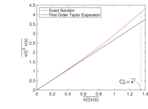
Despite these challenges, the presented MECM method can inexpensively provide with a very good approximation of the system's statistical characteristics as shown in Fig. 4. In particular in Fig. 4, we present the response variance as the intensity of the excitation varies for two cases of the system's parameters. We also compare our results with direct Monte-Carlo simulations and with a standard Gaussian closure method (Sobczyk, 2001; Soong and Grigoriu, 1993; Grigoriu, 2002). For the application of the MECM method we employ the pdf representation (Eq. 11).
Fig. 4: Mean square displacement with respect to the amplification factor of Pierson-Moskowitz spectrum for bistable system with two
different system parameters. (a) λ=1, k1=−1, and k3=1. (b) 0.5
=
λ , k1=−0.5, and k3=1.
We observe that for very large values of q the computed approximation closely follows the Monte-Carlo simulation. On the other hand, the Gaussian closure method systematically underestimates the variance of the response. For lower intensities of the excitation, the exact (Monte-Carlo) variance presents a non-monotonic behavior with respect to q due to the co-existence of the cross- and intra-well oscillations. While the Gaussian closure has very poor performance on capturing this trend, the MECM method can still provide with a satisfactory approximation of the dynamics. Note that the non-smooth transition observed in the MECM curve is due to the fact that for very low values of q the minimization of the cost function (Eq. 28) does not reach a zero value while this is the case for larger values of q . In other words, in the strongly nonlinear regime neither the dynamics constraint nor the closure constraint is satisfied exactly, yet this optimal solution provides with a good approximation of the system dynamics.
After we have obtained the unknown parameters γ and
ρ
x,x by minimizing the cost function for each given q , we can then compute in a post-process manner the covariance functions and the joint pdf. More specifically, since a known γ allows for a givenρ
xy (Eq. 29) we can immediately determine Cxy(τ
) by taking the inverse Fourier transform of Sxy found through Eq. (24). The next step is the numerical integration of the closed moment Eq. (23) utilizing the determined valueρ
x,x with initial conditions given by( )
; , (0)=0, =(0) 2 xx
xx x f x dx and C
C
∫
γ ! (31)where the second condition follows from the symmetry properties of
xx
C . Note that we integrate Eq. (23) instead of using the inverse Fourier transform as we did for Cxy(
τ
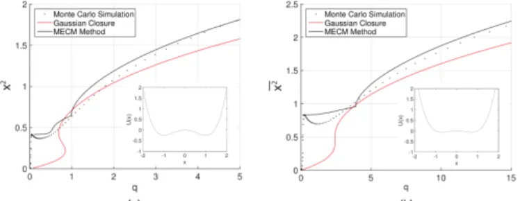
) so that we can impose the variance found by integrating the resulted density for the determined γ. The results as well as a comparison with the Gaussian closure method and a direct Monte-Carlo simulation are presented in Fig. 5. We can observe that through the proposed approach we are able to satisfactorily approximate the correlation function even close to the non-linear regime q=2, where the Gaussian closure method presents important discrepancies.Fig. 5: Correlation functions C and xx Cxy of the bistable system with system parameters λ=1, k1=−1, and k3=1 subjected to
Pierson-Moskowitz spectrum. (a) Amplification factor of q=2 . (b) Amplification factor of q=10.
Finally, using the computed parameters γ and
ρ
x,x we can also approximate the non-Gaussian joint pdf for the response-response-excitation at different time instants. This will be given by), ( ) ( ) ; ( ) ; ( 1 = ) , , ( 1 2 3 ) ( ) ( ) ( xzy f x f z gyexpcxz c yz cxy fxtxt+τyt R γ γ + + (32)
where R is a normalization constant, and the parameters c , 1 c , 2 c 3 are found by expanding the corresponding moments in a Taylor expansion, i.e. through the approximations:
( ) ( )
, = ) , , ( = ) ( xzf()( )() xz ydxdydz c1x22 c12 Cxxτ∫∫∫
xtxt+τyt +O (33)( )
, = ) , , ( = ) ( yzf()( )() xzydxdydz c2x2y2 c22 Cxyτ∫∫∫
xtxt+τ yt +O (34)( )
. = ) , , ( = (0) xyf()( )()xzydxdydz c3x2y2 c32 Cxy∫∫∫
xtxt+τ yt +O (35)If necessary higher order terms may be retained in the Taylor expansion although for the present problem a linear approximation was sufficient. The computed approximation is presented in Fig. 6 through two dimensional marginals as well as through isosurfaces of the full three-dimensional joint pdf. We compare with direct Monte-Carlo simulations and as we are able to observe, the computed pdf closely approximates the expensive Monte-Carlo simulation. We emphasize that in order to accurately capture the joint statistics using the Monte-Carlo approach we had to use 107 number of samples. On the other hand the computational cost through the MECM method is trivial.
Fig. 6: Joint pdf fx(t)x(t+τ)y(t)(x,z,y) computed using the MECM method and direct Monte-Carlo simulations. The system parameters are given by λ=1, k1=−1, and k3=0.3 and the excitation is Gaussian following a Pierson-Moskowitz spectrum with q=20. The pdf is presented through two dimensional marginals as well as through isosurfaces. (a) τ=3. (b) τ=10.
CONCLUSIONS
We have considered the problem of determining the non-Gaussian steady state statistical structure of bistable nonlinear vibrational systems subjected to colored noise excitation. We first derived moment equations that describe the dynamics governing the two-time statistics. We then combined those with a non-Gaussian pdf representation for the joint response-excitation statistics. This representation has i) single time statistical structure consistent with the analytical solutions of the Fokker-Planck equation, and ii) two-time statistical structure with Gaussian characteristics. Using this pdf representation we derived a closure scheme which we formulated in terms of a consistency condition involving the second order statistics of the response, the closure constraint. A similar condition was derived directly through moment equations, the dynamics constraint. We then formulated the two constraints as a low-dimensional minimization problem with respect to the unknown parameters of the representation. The minimization of both the dynamics constraint and the closure constraint imposes an interplay between these two factors in order to obtain a solution that satisfies both constraints as closely as possible. We then applied the presented method to a nonlinear oscillator in the context of ocean wave energy harvesting, which is a single degree of freedom (SDOF) bistable oscillator with linear damping. For the application, it was assumed that the stationary stochastic excitation has a power spectral density given by the Pierson-Moskowitz spectrum. We have shown that the presented method can provide with a very good approximation of the systems second order statistics, when compared with direct Monte-Carlo simulations, even in essentially nonlinear regimes, where Gaussian closure techniques fail completely to capture the dynamics. In addition we can compute, in a post-process manner the full (non-Gaussian) probabilistic structure of the solution. We emphasize that the computational cost associated with the new method is considerably smaller compared with methods that evolve the pdf of the solution since it relies on the minimization of a function with a few unknown variables.
These results indicate that the new method can be a very good candidate when it comes to the calculation of the stochastic response for vibrational system with complex potentials as it is required in parameter optimization or selection. Future endeavors include the application of the presented approach in higher dimensional contexts involving nonlinear energy harvesters and passive protection of structures as well as on the development/optimization of structural configurations able to operate effectively under intermittent loads (Mohamad and Sapsis, 2015).
ACKNOWLEDGMENTS
The authors would like to acknowledge the support from Samsung Scholarship Program as well as the MIT Energy Initiative for support under the grant ‘Nonlinear Energy Harvesting From Broad-Band Vibrational Sources By Mimicking Turbulent Energy Transfer Mechanisms’. T.P.S. is also grateful to the American Bureau of Shipping for support under a Career Development Chair.
REFERENCES
Athanassoulis, GA, Tsantili, IC, and Kapelonis ZG (2013). “Two-time, response-excitation moment equations for a cubic half-oscillator under Gaussian and cubic-Gaussian colored excitation. Part 1: The monostable case”. In: arXiv preprint arXiv:1304.2195.
Barton, DA, Burrow, SG, and Clare LR (2010). “Energy harvesting from vibrations with a nonlinear oscillator”. In: Journal of Vibration and Acoustics 132(2), p. 021009.
Beran, J (1994). Statistics for long-memory processes. Vol. 61. CRC Press.
Bover, D (1978). “Moment equation methods for nonlinear stochastic systems”. In: Journal of Mathematical Analysis and Applications 65(2) pp. 306-320.
Caughey, T (1963). “Equivalent linearization techniques”. In: The Journal of the Acoustical Society of America 35(11) pp. 1706-1711. Caughey, T (1959). “Response of a nonlinear string to random loading”.
In: Journal of Applied Mechanics 26(3), pp. 341-344.
Cho, H, Venturi, D, and Karniadakis, GE (2013). “Adaptive discontinuous Galerkin method for response-excitation PDF equations”. In: SIAM Journal on Scientific Computing 35(4), B890-B911.
Crandall, D, Felzenszwalb, P, and Huttenlocher, D (2005). “Spatial priors for part-based recognition using statistical models”. In: Computer Vision and Pattern Recognition, CVPR 2005. IEEE Computer Society Conference on. Vol. 1. IEEE. pp. 10-17.
Crandall, SH (1980). “Non-Gaussian closure for random vibration of non-linear oscillators”. In: International Journal of Non-Linear Mechanics 15(4), pp. 303-313.
Crandall, SH (1985). “Non-Gaussian closure techniques for stationary random vibration”. In: International journal of non-linear mechanics 20(1), pp. 1-8.
Daqaq, MF (2011). “Transduction of a bistable inductive generator driven by white and exponentially correlated Gaussian noise”. In: Journal of Sound and Vibration 330(11), pp. 2554- 2564.
Daqaq, MF (2012). “On intentional introduction of stiffness nonlinearities for energy harvesting under white Gaussian excitations”. In: Nonlinear Dynamics 69(3), pp. 1063-1079.
Paola, MDi and So, A (2002). “Approximate solution of the Fokker-Planck-Kolmogorov equation”. In: Probabilistic Engineering Mechanics 17(4), pp. 369-384.
Dunne, J and Ghanbari, M (1997). “Extreme-value prediction for non-linear stochastic oscillators via numerical solutions of the stationary FPK equation”. In: Journal of Sound and Vibration 206(5), pp. 697-724.
Dykman, M, Soskin, S, and Krivoglaz, M (1985). “Spectral distribution of a nonlinear oscillator performing Brownian motion in a double-well potential”. In: Physica A: Statistical Mechanics and its Applications 133(1), pp. 53-73.
Dykman, M et al (1988). “Spectral density of fluctuations of a double-well Duffing oscillator driven by white noise”. In: Physical Review A 37(4), p. 1303.
Ferrari, M et al (2010). “Improved energy harvesting from wideband vibrations by nonlinear piezoelectric converters”. In: Sensors and Actuators A: Physical 162(2), pp. 425-431.
Gammaitoni, L, Neri, I and Vocca, H (2009). “Nonlinear oscillators for vibration energy harvesting”. In: Applied Physics Letters 94(16), p. 164102.
Green, P, Papatheou, E and Sims, ND (2013). “Energy harvesting from human motion and bridge vibrations: An evaluation of current nonlinear energy harvesting solutions”. In: Journal of Intelligent Material Systems and Structures.
Green, P et al (2012). “The benefits of Duffing-type nonlinearities and electrical optimization of a mono-stable energy harvester under white Gaussian excitations". In: Journal of Sound and Vibration 331(20), pp. 4504-4517.
Grigoriu, M (1991). “A consistent closure method for non-linear random vibration”. In: International journal of non-linear mechanics 26(6), pp. 857-866.
Grigoriu, M (1999). “Moment closure by Monte Carlo simulation and moment sensitivity factors”. In: International journal of non-linear mechanics 34(4), pp. 739-748.
Grigoriu, M (2002). Stochastic calculus: applications in science and engineering. Springer.
Halvorsen, E (2013). “Fundamental issues in nonlinear wideband-vibration energy harvesting”. In: Physical Review E 87(4), p. 042129. Harne, R and Wang, K (2013). “A review of the recent research on
vibration energy harvesting via bistable systems”. In: Smart Materials and Structures 22(2), p. 023001.
Hasofer, A and Grigoriu, M (1995). “A new perspective on the moment closure method”. In: Journal of applied mechanics 62(2), pp. 527-532. He, Q and Daqaq, MF (2014). “New Insights into Utilizing Bi-stability
for Energy Harvesting under White Noise”. In: Journal of Vibration and Acoustics.
Ibrahim, R, Soundararajan, A and Heo, H (1985). “Stochastic response of nonlinear dynamic systems based on a non-Gaussian closure”. In: Journal of applied mechanics 52(4), pp. 965-970.
Isserlis, L (1918). “On a formula for the product-moment coefficient of any order of a normal frequency distribution in any number of variables”. In: Biometrika, pp. 134-139.
Iyengar, R and Dash, P (1978). “Study of the random vibration of nonlinear systems by the Gaussian closure technique”. In: Journal of Applied Mechanics 45(2), pp. 393-399.
Joo, HK and Sapsis, TP (2014). “Performance measures for single-degree-of-freedom energy harvesters under stochastic excitation”. In: Journal of Sound and Vibration 333(19), pp. 4695-4710.
Kazakov, I (1954). “An approximate method for the statistical investigation of nonlinear systems”. In: Trudy VVIA im Prof. NE Zhukovskogo 394, pp. 1-52.
Kluger, JM, Sapsis, TP and Slocum, AH (2015). “Robust energy
harvesting from walking vibrations by means of nonlinear cantilever beams”. In: Journal of Sound and Vibration.
Liu, Q and Davies, HG (1988). “Application of non-Gaussian closure to the nonstationary response of a Duffing oscillator". In: International journal of non-linear mechanics 23(3), pp. 241-250.
Mann, B and Sims, ND (2009). “Energy harvesting from the nonlinear oscillations of magnetic levitation”. In: Journal of Sound and Vibration 319(1), pp. 515-530.
Mohamad, M and Sapsis, TP (2015). “Robust energy harvesting from walking vibrations by means of nonlinear cantilever beams”. In: SIAM Journal of Uncertainty Quantification, Submitted.
Naess, A and Moan, T (2012). Stochastic dynamics of marine structures. Cambridge University Press.
Noori, M, Saffar, A, and Davoodi, H (1987). “A comparison between non-Gaussian closure and statistical linearization techniques for random vibration of a nonlinear oscillator”. In: Computers & structures 26.6, pp. 925-931.
Roberts, JB and Spanos, PD (2003). Random vibration and statistical linearization. Courier Dover Publications.
Sancho, N (1970). “Technique for nding the moment equations of a nonlinear stochastic system”. In: Journal of Mathematical Physics 11(3), pp. 771-774.
Sapsis, TP and Athanassoulis, GA (2008). “New partial differential equations governing the joint, response-excitation, probability distributions of nonlinear systems, under general stochastic excitation”. In: Probabilistic Engineering Mechanics 23(2), pp. 289-306.
Sobczyk, K (2001). Stochastic differential equations: with applications to physics and engineering. Vol. 40. Springer.
Socha, L (2008). Linearization methods for stochastic dynamic systems. Vol. 730. Springer.
Soize, C (1994). The Fokker-Planck equation for stochastic dynamical systems and its explicit steady state solutions. Vol. 17. World Scientific. Soong, TT and Grigoriu, M (1993). “Random vibration of mechanical
and structural systems”. In: NASA STI/Recon Technical Report A 93, p. 14690.
Stratonovich, RL (1967). Topics in the theory of random noise. Vol. 2. CRC Press.
To, CW (2011). Nonlinear random vibration: Analytical techniques and applications. CRC Press.
Venturi, D et al (2012). “A computable evolution equation for the joint response-excitation probability density function of stochastic dynamical systems”. In: Proceedings of the Royal Society A: Mathematical, Physical and Engineering Science 468(2139), pp. 759-783.
Wojtkiewicz, S, Spencer Jr, B, and Bergman, L (1996). “On the cumulant-neglect closure method in stochastic dynamics”. In: International journal of non-linear mechanics 31(5), pp. 657-684. Wojtkiewicz, S et al (1999). “Response of stochastic dynamical systems
driven by additive Gaussian and Poisson white noise: Solution of a forward generalized Kolmogorov equation by a spectral finite difference method”. In: Computer methods in applied mechanics and engineering 168(1), pp. 73-89.
Wu, W and Lin, Y (1984). “Cumulant-neglect closure for non-linear oscillators under random parametric and external excitations”. In: International Journal of Non-Linear Mechanics 19(4), pp. 349-362.