Steganalysis by Subtractive Pixel Adjacency Matrix

HAL Id: hal-00541410

https://hal.archives-ouvertes.fr/hal-00541410

Submitted on 30 Nov 2010

HAL is a multi-disciplinary open access

archive for the deposit and dissemination of

sci-entific research documents, whether they are

pub-lished or not. The documents may come from

teaching and research institutions in France or

abroad, or from public or private research centers.

L’archive ouverte pluridisciplinaire HAL, est

destinée au dépôt et à la diffusion de documents

scientifiques de niveau recherche, publiés ou non,

émanant des établissements d’enseignement et de

recherche français ou étrangers, des laboratoires

publics ou privés.

Tomas Pevny, Patrick Bas, Jessica Fridrich

To cite this version:

Tomas Pevny, Patrick Bas, Jessica Fridrich. Steganalysis by Subtractive Pixel Adjacency Matrix.

IEEE Transactions on Information Forensics and Security, Institute of Electrical and Electronics

En-gineers, 2010, 5 (2), pp.215–224. �hal-00541410�

Steganalysis by Subtractive Pixel Adjacency

Matrix

Tomáš Pevný and Patrick Bas and Jessica Fridrich, IEEE member

Abstract

This paper presents a method for detection of steganographic methods that embed in the spatial domain by adding a low-amplitude independent stego signal, an example of which is LSB matching. First, arguments are provided for modeling the differences between adjacent pixels using first-order and second-order Markov chains. Subsets of sample transition probability matrices are then used as features for a steganalyzer implemented by support vector machines.

The major part of experiments, performed on four diverse image databases, focuses on evaluation of detection of LSB matching. The comparison to prior art reveals that the presented feature set offers superior accuracy in detecting LSB matching.

Even though the feature set was developed specifically for spatial domain steganalysis, by constructing steganalyzers for ten algorithms for JPEG images it is demonstrated that the features detect steganography in the transform domain as well.

I. INTRODUCTION

A large number of practical steganographic algorithms performs embedding by applying a mutually indepen-dent embedding operation to all or selected elements of the cover [8]. The effect of embedding is equivalent to adding to the cover an independent noise-like signal called the stego noise. A popular method falling under this paradigm is the Least Significant Bit (LSB) replacement, in which LSBs of individual cover elements are replaced with message bits. In this case, the stego noise depends on cover elements and the embedding operation is LSB flipping, which is asymmetrical. It is exactly this asymmetry that makes LSB replacement easily detectable [16], [18], [19]. A trivial modification of LSB replacement is LSB matching (also called

Tomáš Pevný and Patrick Bas are supported by the National French projects Nebbiano ANR-06-SETIN-009, ANR-RIAM Estivale, and ANR-ARA TSAR. The work of Jessica Fridrich was supported by Air Force Office of Scientific Research under the research grants FA9550-08-1-0084 and FA9550-09-1-0147. The U.S.Government is authorized to reproduce and distribute reprints for Governmental purposes notwithstanding any copyright notation there on. The views and conclusions contained herein are those of the authors and should not be interpreted as necessarily representing the official policies, either expressed or implied of AFOSR or the U.S.Government.

The authors would like to thank Mirek Goljan for providing code for extraction of WAM features, Gwenaël Doërr for sharing the code to extract ALE features, and Jan Kodovský for providing the database of stego images for YASS.

Tomáš Pevný is presently a researcher at Czech Technical University in Prague, FEE, Department of Cybernetics, Agent Technology Center (e-mail: pevnak@gmail.com). The majority of the work presented in this paper has been done during his post-doctorant stay at Gipsa-Lab, INPG - Gipsa-Lab , Grenoble, France

Patrick Bas is a senior researcher at Gipsa-lab, INPG - Gipsa-Lab , Grenoble, France (e-mail:patrick.bas@gipsa-lab.inpg.fr)

Jessica Fridrich is a Professor at the Department of Electrical and Computer Engineering, Binghamton University, NY 13902 USA (607-777-6177; fax: 607-777-4464; e-mail: fridrich@binghamton.edu)

±1 embedding), which randomly increases or decreases pixel values by one to match the LSBs with the communicated message bits. Although both steganographic schemes are very similar in that the cover elements are changed by at most one and the message is read from LSBs, LSB matching is much harder to detect. Moreover, while the accuracy of LSB replacement steganalyzers is only moderately sensitive to the cover source, most current detectors of LSB matching exhibit performance that varies significantly across different cover sources [20], [4].

One of the first heuristic detectors of embedding by noise adding used the center of gravity of the Histogram Characteristic Function [11], [17], [26] (HCF). A rather different heuristic approach was taken in [36], where the quantitative steganalyzer of LSB matching was based on maximum likelihood estimation of the change rate. Alternative methods used features extracted as moments of noise residuals in the wavelet domain [13], [10] and statistics of Amplitudes of Local Extrema in the graylevel histogram [5] (further called the ALE detector). A recently published experimental comparison of these detectors [20], [4] shows that the Wavelet Absolute Moments (WAM) steganalyzer [10] is the most accurate and versatile, offering an overall good performance on diverse images.

The heuristic behind embedding by noise adding is based on the fact that during image acquisition many noise sources are superimposed on the acquired image, such as the shot noise, readout noise, amplifier noise, etc. In the literature on digital imaging sensors, these combined noise sources are usually modeled as an iid signal largely independent of the content. While this is true for the raw sensor output, subsequent in-camera processing, such as color interpolation, denoising, color correction, and filtering, introduces complex dependences into the noise component of neighboring pixels. These dependences are violated by steganographic embedding where the stego noise is an iid sequence independent of the cover image, opening thus door to possible attacks. Indeed, most steganalysis methods in one way or another try to use these dependences to detect the presence of the stego noise.

The steganalysis method described in this paper exploits the independence of the stego noise as well. By modeling the differences between adjacent pixels in natural images, the method identifies deviations from this model and postulates that such deviations are due to steganographic embedding. The steganalyzer is constructed as follows. A filter suppressing the image content and exposing the stego noise is applied. Dependences between neighboring pixels of the filtered image (noise residuals) are modeled as a higher-order Markov chain. The sample transition probability matrix is then used as a vector feature for a feature-based steganalyzer implemented using machine learning algorithms.

The idea to model differences between pixels by Markov chains was proposed for the first time in [37]. In [41], it was used to attack embedding schemes based on spread spectrum and quantization index modulation and LSB replacement algorithms. The same technique was used in [34] to model dependences between DCT coefficients to attack JPEG steganographic algorithms. One of the major contribution of our work is the use of higher-order Markov chains, exploiting of symmetry in natural images to reduce the dimensionality of the extracted features, proper justification of the model, and exhaustive evaluation of the method. Although the presented steganalytic method is developed and verified for grayscale images, it can be easily extended to color images by creating a specialized classifier for each color plane and fusing their outputs by means of ensemble methods.

This paper expands on our previously published work on this topic [28]. The novel additions include experimental evaluation of the proposed steganalytic method on algorithms hiding in the transform (DCT) domain, comparison of intra- and inter-database errors, steganalysis of YASS [35], [33], and a more thorough theoretical explanation of the benefits of using the pixel-difference model of natural images.

This paper is organized as follows. Section II starts with a description of the filter used to suppress the image content and expose the stego noise. It continues with the calculation of the features as the sample transition probability matrix of a higher-order Markov model of the filtered image. Section III briefly describes the rest of the steganalyzer construction, which is the training of a support vector machine classifier. The subsequent Section IV presents the major part of experiments consisting of (1) comparison of several versions of the feature set differing in the range of modeled differences and the degree of the Markov model, (2) estimation of intra-and inter-database errors on four diverse image databases, intra-and (3) comparison to prior art. In Section V it is shown that the presented feature set is also useful for detecting steganography in block-transform DCT domain (JPEG images). The paper is concluded in Section VI.

II. SUBTRACTIVEPIXELADJACENCYMATRIX

A. Rationale

In principle, higher-order dependences between pixels in natural images can be modeled by histograms of pairs, triples, or larger groups of neighboring pixels. However, these histograms possess several unfavorable aspects that make them difficult to be used directly as features for steganalysis:

1) The number of bins in the histograms grows exponentially with the number of pixels. The curse of dimensionality may be encountered even for the histogram of pixel pairs in an 8-bit grayscale image (2562_{= 65536 bins).}

2) The estimates of some bins may be noisy because they have a very low probability of occurrence, such as completely black and completely white pixels next to each other.

3) It is rather difficult to find a statistical model for pixel groups because their statistics are influenced by the image content. By working with the noise component of images, which contains the most energy of the stego noise signal, we increase the SNR and, at the same time, obtain a tighter model. 1

The second point indicates that a good model should capture those characteristics of images that can be robustly estimated. The third point indicates that some pre-processing, such as denoising or calibration, should be applied to increase the SNR. An example of this step is working with a noise residual as in WAM [10].

Representing a grayscale m × n image with a matrix

{Ii,j|Ii,j ∈ {0, 1, 2, . . . , 255},

i_{∈ {1, . . . , m}, j ∈ {1, . . . , n}}}

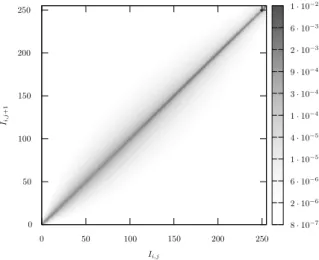
Figure 1 shows the probability Pr(Ii,j, Ii,j+1) of occurrence of two horizontally adjacent pixels (Ii,j, Ii,j+1)

estimated from approximately 10700 8-bit grayscale images from the BOWS2 database. Due to high spatial correlation in natural images, the colors of neighboring pixels are similar, a fact that shapes the probability

8 · 10−7 2 · 10−6 6 · 10−6 1 · 10−5 4 · 10−5 1 · 10−4 3 · 10−4 9 · 10−4 2 · 10−3 6 · 10−3 1 · 10−2 0 0 50 50 100 100 150 150 200 200 250 250 Ii,j Ii,j +1

Figure 1. Distribution of two horizontally adjacent pixels (Ii,j, Ii,j+1)in 8-bit grayscale images estimated from approximately 10700

images from the BOWS2 database (see Section IV for more details about the database). The degree of gray at (x, y) is the probability Pr(Ii,j= x∧ Ii,j+1= y)at the logarithmic scale.

−8 −6 −4 −2 0 2 4 6 8 −10 −9 −8 −7 Ii,j− Ii+1,j log [P r( Ii,j − Ii+1 ,j )] Ii,j= 64 Ii,j= 128 Ii,j= 196

Figure 2. Probability Pr(Ii,j− Ii,j+1|Ii,j)(horizontal cuts of the graph shown in Figure 1) for Ii,j= 64, Ii,j= 128,and Ii,j= 196

in 8-bit grayscale images estimated from approximately 10700 images from the BOWS2 database (see Section IV for more details about the database).

distribution into a ridge that follows the major diagonal. A close inspection of Figure 1 suggests that the profile of the ridge along the major diagonal does not change much with the pixel value. This observation is confirmed in Figure 2 showing the ridge profile at three locations Ii,j = {64, 128, 196}. The fact that the profile shape

is approximately constant (it starts deviating only for high intensity pixels Ii,j = 196) suggests that the pixel

difference Ii,j+1− Ii,j is approximately independent of Ii,j. We quantified this statement by evaluating the

Because

I(Ii,j+1− Ii,j, Ii,j) = H(Ii,j+1− Ii,j) − H(Ii,j+1− Ii,j|Ii,j)

= H(Ii,j+1− Ii,j) − H(Ii,j+1|Ii,j),

the mutual information can be estimated by evaluating the two entropy terms from their corresponding defini-tions:

H(Ii,j+1− Ii,j) = 4.6757

H(Ii,j+1|Ii,j) = 4.5868,

yielding to I(Ii,j+1− Ii,j, Ii,j) = 8.89 · 10−2. Thus, knowing Ii,j the entropy of the difference Ii,j+1− Ii,j

decreases only by 0.0889/4.68 = 2%, which shows that any dependence between the pixel differences Ii,j+1−

Ii,j and pixel values Ii,j is fairly small.2

The arguments above allow us to model the pixels in natural images by working with the differences Ii,j+1−

Ii,j instead of the co-occurrences (Ii,j+1, Ii,j), which greatly reduces the model dimensionality from 65536

to 511 in an 8-bit grayscale image. It is, however, still impossible to model the differences using a Markov chain as the transition probability matrix would have 5112 _{elements. Further simplification and reduction can}

be achieved by realizing that, for the purpose of blind steganalysis, the statistical quantities estimated from pixels have to be estimable even from small images. Hence, only pixel pairs close to the ridge, alternatively, with pairs with a small difference Ii,j+1− Ii,j ∈ [−T, T ], are relevant for steganalysis. This approach was

already pursued in [37], where probabilities of selected pixel pairs were used as steganalytic features. B. The SPAM features

We now explain the Subtractive Pixel Adjacency Model (SPAM) that will be used to compute the features for steganalysis. The reference implementation is available for free download on http://dde.binghamton.edu/ download/spam/. First, the transition probabilities along eight directions are computed.3 _{The differences and}

the transition probability are always computed along the same direction. We explain further calculations only on the horizontal direction as the other directions are obtained in a similar manner. All direction-specific quantities will be denoted by a superscript {←, →, ↓, ↑, �, �, �, �} showing the direction of the calculation.

The calculation of features starts by computing the difference array D·_{.For a horizontal direction left-to-right}

D→

i,j= Ii,j− Ii,j+1,

i_{∈ {1, . . . , m}, j ∈ {1, . . . , n − 1}.}

As introduced in Section II-A, the first-order SPAM features, F1st_{, model the difference arrays D by a}

first-order Markov process. For the horizontal direction, this leads to

M→

u,v= P r(D→i,j+1= u|D→i,j= v),

2_{Following a similar reasoning, Huang et al. [15] estimated the mutual information between Ii,j− Ii,j+1and Ii,j+ Ii,j+1to 0.0255.} 3_{There are four axes: horizontal, vertical, major and major diagonal, and two directions along each axis, which leads to eight directions}

Order T Dimension 1st _{4 162}

1st _{8 578}

2nd _{3 686}

Table I

DIMENSION OF MODELS USED IN OUR EXPERIMENTS. THE COLUMN“ORDER”SHOWS THE ORDER OF THEMARKOV CHAIN ANDTIS

THE RANGE OF DIFFERENCES.

where u, v ∈ {−T, . . . , T }. If P r(D→

i,j= v) = 0 then M→u,v= P r(D→i,j+1= u|D→i,j= v) = 0.

The second-order SPAM features, F2nd_{, model the difference arrays D by a second-order Markov process.}

Again, for the horizontal direction,

M→

u,v,w = P r(D→i,j+2 = u|D→i,j+1 = v, D→i,j= w),

where u, v, w ∈ {−T, . . . , T }. If P r(D→

i,j+1 = v, D→i,j = w) = 0 then M→u,v,w = P r(D→i,j+2 = u|D→i,j+1 =

v, D→

i,j= w) = 0.

To decrease the feature dimensionality, we make a plausible assumption that the statistics in natural images are symmetric with respect to mirroring and flipping (the effect of portrait / landscape orientation is negligible). Thus, we separately average the horizontal and vertical matrices and then the diagonal matrices to form the final feature sets, F1st_{, F}2nd_{. With a slight abuse of notation, this can be formally written:}

F· 1,...,k = 1 4 � M→ · + M←· + M↓· + M↑· � , F· k+1,...,2k = 1 4 �_M� · + M�· + M�· + M�· � , (1)

where k = (2T +1)2_{for the first-order features and k = (2T +1)}3_{for the second-order features. In experiments}

described in Section IV, we used T = 4 and T = 8 for the first-order features, obtaining thus 2k = 162, 2k = 578 features, and T = 3 for the second-order features, leading to 2k = 686 features (c.f., Table I).

Figure 3 summarizes the extraction process of SPAM features. The features are formed by the average sample Markov transition probability matrices (1) in the range [−T, T ]. The complexity of the model is determined by the order of the Markov model and by the range of differences T .

The calculation of the difference array can be interpreted as high-pass filtering with the kernel [−1, +1], which is, in fact, the simplest edge detector. The filtering suppresses the image content and exposes the stego noise, which results in a higher SNR. The idea of using filtering to enhance signal to noise ratio in steganalysis has been already used, for example, in the WAM features calculating moments from noise residual in Wavelet domain and it implicitly appeared in the construction of Farid’s features [6] and in [40]. The filtering can also be seen as a different form of calibration [7]. From this point of view, it would make sense to use more sophisticated filters with a better SNR. Interestingly, none of the filters we tested4 _{provided consistently better}

4_{We experimented with the adaptive Wiener filter with 3 × 3 neighborhood, the wavelet filter [27] used in WAM, and discrete filters,}

2 6 6 4 0 +1 0 +1 −4 +1 0 +1 0 3 7 7 5 , [+1, −2, +1], and [+1, +2, −6, +2, +1].

Difference filter

Markov chain

Features

Threshold T

Chain order

Figure 3. Schema of extraction of SPAM features.

performance. This is likely due to the fact that the averaging caused by more sophisticated filters distorts the statistics of the stego noise, which results in worse detection accuracy. The [−1, 1] filter is also a projection of the pixel values co-occurrence matrix on one of the independent directions — the anti-diagonal.

III. EVALUATIONPROCEDURE

The construction of steganalyzers based on SPAM features relies on pattern-recognition classifiers. All ste-ganalyzers presented in this paper were constructed by using soft-margin Support Vector Machines (SVMs) [38] with the Gaussian kernel k(x, y) = exp�−γ�x − y�2

2

�

, γ > 0.Since the construction and subsequent evaluation of steganalyzers always followed the same procedure, the procedure is described here to avoid tedious repetition later.

Let us assume that the set of stego images available for the experiment was created from some set of cover images and that both sets of images are available for the experiment. Prior to all experiments, the images are divided into a training and testing set of equal size, so that the cover image and the corresponding stego image is either in the training or in the testing set. In this way, it is ensured that images in the testing set used to estimate the error of steganalyzers were not used in any form during training.

Before training the soft-margin SVM on the training set, the value of the penalization parameter C and the kernel parameter γ need to be set. These hyper-parameters balance the complexity and accuracy of the classifier. The hyper-parameter C penalizes the error on the training set. Higher values of C produce classifiers more accurate on the training set but also more complex with a possibly worse generalization.5 _{On the other hand,}

a smaller value of C produces simpler classifiers with worse accuracy on the training set but hopefully with better generalization. The role of the kernel parameter γ is similar to C. Higher values of γ make the classifier more pliable but likely prone to over-fitting the data, while lower values of γ have the opposite effect.

The values of C and γ should be chosen to give the classifier the ability to generalize. The standard approach is to estimate the error on unknown samples using cross-validation on the training set on a fixed grid of values and then select the value corresponding to the lowest error (see [14] for details). In this paper, we used five-fold cross-validation with the multiplicative grid

C _{∈ {0.001, 0.01, . . . , 10000},}

γ ∈ {2i

|i ∈ {−d − 3, . . . , −d + 3},

where d is the number of features in the subset.

The steganalyzer performance is always evaluated on the testing set using the minimal average decision error under equal probability of cover and stego images

PErr=

1

2(PFp+ PFn) , (2)

where PFp and PFn stand for the probability of false alarm or false positive (detecting cover as stego) and

probability of missed detection (false negative).

IV. DETECTION OFLSB MATCHING

To evaluate the performance of the proposed feature sets, we subjected them to extensive tests on a well-known archetype of embedding by noise adding – the LSB matching. First, we constructed and compared steganalyzers using first-order Markov chain features with differences in the range [−4, +4] and [−8, +8] (further called first-order SPAM features) and second-order Markov chain features with differences in the range [−3, +3] (further called second-order SPAM features) on four different image databases. Then, we compared the SPAM steganalyzers to prior art, namely to detectors based on WAM [10] and ALE [5] features. We also investigated the problem of training the steganalyzer on images coming from a different database than images in the testing set (inter-database error).

1) Image databases: It is a well known fact that the accuracy of steganalysis may vary significantly across different cover sources. In particular, images with a large noise component, such as scans of photographs, are much more challenging for steganalysis than images with a low noise component or filtered images (JPEG compressed). In order to assess the SPAM models and compare them to prior art under different conditions, we measured their accuracy on the following four databases

1) CAMERA contains approximately 9200 images with sizes in the range between 1Mpix and 6Mpix captured by 23 different digital cameras in the raw format and converted to grayscale.

2) BOWS2 contains approximately 10700 grayscale images with fixed size 512 × 512 coming from rescaled and cropped natural images of various sizes. This database was used during the BOWS2 contest [3]. 3) NRCS consists of 1576 raw scans of film converted to grayscale with fixed size 2100 × 1500 [1]. 4) JPEG85 contains 9200 images from CAMERA compressed by JPEG with quality factor 85. 5) JOINT contains images from all four databases above, approximately 30800 images.

In each database, two sets of stego images were created with payloads 0.5 bits per pixel (bpp) and 0.25 bpp. According to the recent evaluation of steganalytic methods of LSB matching [4], these two embedding rates are already difficult to detect reliably. These two embedding rates were also used in [10].

A. Order of Markov Chains

This paragraph compares the accuracy of steganalyzers created as described in Section III employing the first-order SPAM features with T = 4 and T = 8, and second-order SPAM features with T = 3. The reported errors (2), measured on images from the testing set, are intra-database errors, which means that the images in the training and testing set came from the same database.

T bpp CAMERA BOWS2 JPEG85 NRCS 1st SPAM 4 0.25 0.097 0.098 0.021 0.216 1st SPAM 8 0.25 0.103 0.123 0.033 0.226 2nd SPAM 3 0.25 0.057 0.055 0.009 0.167 1st SPAM 4 0.5 0.045 0.040 0.007 0.069 1st SPAM 8 0.5 0.052 0.052 0.012 0.093 2nd SPAM 3 0.5 0.027 0.024 0.002 0.069 Table II

MINIMAL AVERAGE DECISION ERROR(2)OF STEGANALYZERS IMPLEMENTED USINGSVMS WITHGAUSSIAN KERNELS ON IMAGES

FROM THE TESTING SET. THE LOWEST ERROR FOR A GIVEN DATABASE AND MESSAGE LENGTH IS IN BOLDFACE.

T bpp CAMERA BOWS2 JPEG85 NRCS 1st SPAM 4 0.25 11:44:16 17:55:21 05:56:57 00:21:18 1st SPAM 8 0.25 23:30:26 32:23:38 19:16:44 00:40:10 2nd SPAM 3 0.25 20:10:26 23:50:38 14:47:40 00:47:54 1st SPAM 4 0.5 07:50:51 10:02:11 03:58:16 00:14:02 1st SPAM 8 0.5 21:44:36 20:18:07 12:44:56 00:31:25 2nd SPAM 3 0.5 19:01:15 19:25:09 09:55:02 00:42:10 Table III

TIME IN HH:MM:SS TO PERFORM THE GRID-SEARCH TO FIND SUITABLE PARAMETERS FOR TRAINING OFSVMCLASSIFIERS.

The results, summarized in Table II, show that steganalyzers employing the second-order SPAM features that model the pixel differences in the range [−3, +3] are always the best. First, notice that increasing the model scope by enlarging T does not result in better accuracy as first-order SPAM features with T = 4 produce more accurate steganalyzers than first-order SPAM features with T = 8. We believe that this phenomenon is due to the curse of the dimensionality, since first-order SPAM features with T = 4 have dimension 162, while first-order SPAM features with T = 8 have dimension 578. The contribution to the classification of additional features far from the center of the ridge is probably not very large and it is outweighted by the increased number of features. It is also possible that the added features are simply not informative and deceptive. On the other hand, increasing the order of the Markov chain (using second-order SPAM features) proved to be highly beneficial as the accuracy of the resulting steganalyzers has significantly increased, despite having the highest dimension.

In the rest of this paragraph, we discuss the time needed to train the SVM classifier and to perform the classification. In theory, the complexity of training an SVM classifier grows with the cube of the number of training samples and linearly with the number of features. On the other hand, state-of-the-art algorithms train SVMs using heuristics to considerably speed up the training. In our experiments, we have observed that the actual time to train a SVM greatly depends on the complexity of the classification problem. SVMs solving an easily separable problem require a small number of support vectors and are thus trained quickly, while training an SVM for highly overlapping features requires a large number of support vectors and is thus very time consuming. The same holds for the classification, whose complexity grows linearly with the number of

T bpp CAMERA BOWS2 JPEG85 NRCS 1st SPAM 4 0.25 09:37 09:38 07:25 00:49 1st SPAM 8 0.25 18:05 14:55 13:22 00:48 2nd SPAM 3 0.25 13:36 18:25 10:39 00:40 1st SPAM 4 0.5 06:33 06:15 04:07 00:16 1st SPAM 8 0.5 11:13 11:28 10:38 00:26 2nd SPAM 3 0.5 15:41 18:30 13:24 00:29 exact Table IV

TIME IN MM:SS TO TRAIN THESVMCLASSIFIER AND TO CLASSIFY ALL SAMPLES FROM THE RELEVANT DATABASE(ALL EXAMPLES

FROM THE TRAINING AND TESTING SET).

support vectors and the number of features.

Tables III, IV show the actual times6 _{to perform grid-search, and to train and evaluate accuracy of the}

classifiers. We can observe a linear dependency on the number of features – the running time of steganalyzers using the first-order SPAM features is approximately two times shorter than the rest. A similar linear dependence is observed for the number of training samples. (Note that the times for the smaller NRCS database are shorter than for the rest.)

B. Inter-database Error

It is well known that steganalysis in the spatial domain is very sensitive to the type of cover images. This phenomenon can be observed in the results presented in the previous section as steganalysis is more accurate on less noisy images (previously JPEG compressed images) than on very noisy images (scanned images from the NRCS database). We can expect this problem to be more pronounced if the images in the training and testing sets come from different databases (inter-database error). The inter-database error reflects more closely the performance of the steganalyzer in real life because the adversary rarely has information about the cover source. This problem was already investigated in [4] using the WAM and ALE features and the HCF detector. In our experiments, we used images from CAMERA, BOWS2, JPEG85, and NRCS. These image sources are very different: NRCS images are very noisy, while JPEG85 images are smoothed by the lossy compression. BOWS2 images are small with a fixed size, while images in CAMERA are large and of varying dimensions.

The training set of steganalyzers consists of 5000 cover and 5000 stego images randomly selected from three databases. The accuracy was evaluated on images from the remaining fourth database, which was not used during training. For testing purposes, we did not use all images from the fourth database, but only images reserved for testing as in the previous two sections to allow fair comparison with the results presented in Table II. All steganalyzers used second-order SPAM features with T = 3 and were created as described in Section III. The error is shown in rows denoted as “Disjoint” in Table V.

The error rates of all eight steganalyzers are summarized in Table V in rows captioned “Disjoint.” Comparing the inter-database errors to the intra-database errors in Table II, we observe a significant drop in accuracy. This drop is expected because of the mismatch between the sources for testing and training as explained above.

bpp CAMERA BOWS2 JPEG85 NRCS Disjoint 0.25 0.3388 0.1713 0.3247 0.3913 Disjoint 0.5 0.2758 0.1189 0.2854 0.3207 Joint 0.25 0.0910 0.0845 0.0198 0.2013 Joint 0.5 0.0501 0.0467 0.0102 0.08213 Table V

INTER-DATABASE ERRORPErrOF STEGANALYZERS EMPLOYING SECOND-ORDERSPAMFEATURES WITHT = 3.THE CAPTION OF

COLUMNS DENOTES THE SOURCE OF TEST IMAGES. THE ROWS CAPTIONED“DISJOINT”SHOW THE ERROR OF STEGANALYZERS

ESTIMATED ON IMAGES FROM THE DATABASE NOT USED TO CREATE THE TRAINING SET(EIGHT STEGANALYZERS IN TOTAL). THE

ROWS CAPTIONED“JOINT”SHOW THE ERROR OF STEGANALYZERS TRAINED ON IMAGES FROM ALL FOUR DATABASES(TWO

STEGANALYZERS IN TOTAL).

If the adversary does not know anything about the cover source, her best strategy is to train the steganalyzer on as diverse image database as possible. To investigate if it is possible to create a steganalyzer based on the SPAM features capable of reliably classifying images from various sources, we created two steganalyzers targeted to a fixed message length trained on 5000 cover and 5000 stego images randomly selected from the training portions of all four databases. The errors are shown in Table V in rows captioned by “Joint.” Comparing their errors to the inter-database errors, we observe a significant increase in accuracy, which means that it is possible to create a single steganalyzer with SPAM features capable of handling diverse images simultaneously. Moreover, the errors are by 0.04 higher than the errors of steganalyzers targeted to a given database (see Table II), which tells us that this approach to universal steganalysis has a great promise.

An alternative approach to constructing a steganalyzer that is less sensitive to the cover image type is to train a bank of classifiers for several cover types and equip this bank with a forensic pre-classifier that would attempt to recognize the cover image type and then send the image to the appropriate classifier. This approach is not pursued in this paper and is left as a possible future effort.

C. Comparison to Prior Art

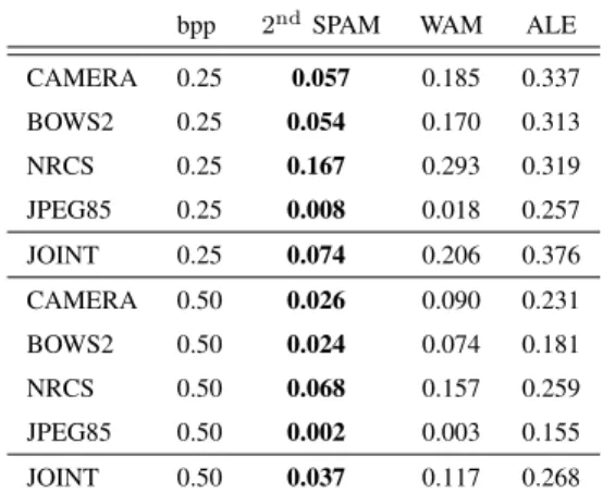
Table VI shows the classification error (2) of the steganalyzers using the second-order SPAM features (686 features), WAM [10] (contrary to the original features, we calculate moments from 3 decomposition levels yielding to 81 features), and ALE [5] (10 features) on all four databases for two relative payloads. We have created a special steganalyzer for each combination of database, features, and payload (total 5 × 3 × 2 = 30 steganalyzers). The steganalyzers were implemented by SVMs with a Gaussian kernel as described in Section III. In all cases, the steganalyzers employing the second-order SPAM features perform the best, the WAM steganalyzers are second with about three times higher error, and ALE steganalyzers are the worst. Figure 4 compares the steganalyzers in selected cases using the Receiver Operating Characteristic (ROC) curve, plotted by varying the threshold of trained SVMs with a Gaussian kernel. The dominant performance of SPAM steganalyzers is quite apparent.

bpp 2nd_{SPAM WAM ALE} CAMERA 0.25 0.057 0.185 0.337 BOWS2 0.25 0.054 0.170 0.313 NRCS 0.25 0.167 0.293 0.319 JPEG85 0.25 0.008 0.018 0.257 JOINT 0.25 0.074 0.206 0.376 CAMERA 0.50 0.026 0.090 0.231 BOWS2 0.50 0.024 0.074 0.181 NRCS 0.50 0.068 0.157 0.259 JPEG85 0.50 0.002 0.003 0.155 JOINT 0.50 0.037 0.117 0.268 Table VI

ERROR(2)OF STEGANALYZERS FORLSBMATCHING WITH MESSAGE LENGTH0.25AND0.5BPP. STEGANALYZERS WERE

IMPLEMENTED ASSVMS WITHGAUSSIAN KERNEL. THE LOWEST ERROR FOR A GIVEN DATABASE AND MESSAGE LENGTH IS IN

BOLDFACE. 0 0.2 0.4 0.6 0.8 1 0 0.2 0.4 0.6 0.8 1

False positive rate

D et ec ti on ac cu rac y 2nd SPAM WAM ALE

(a) CAMERA, Payload = 0.25bpp

0 0.2 0.4 0.6 0.8 1 0 0.2 0.4 0.6 0.8 1

False positive rate

D et ec ti on ac cu rac y 2nd SPAM WAM ALE (b) CAMERA, Payload = 0.50bpp 0 0.2 0.4 0.6 0.8 1 0 0.2 0.4 0.6 0.8 1

False positive rate

D et ec ti on ac cu rac y 2nd SPAM WAM ALE (c) JOINT, Payload = 0.25bpp 0 0.2 0.4 0.6 0.8 1 0 0.2 0.4 0.6 0.8 1

False positive rate

D et ec ti on ac cu rac y 2nd SPAM WAM ALE (d) JOINT, Payload = 0.50bpp

V. STEGANALYSIS OFJPEGIMAGES

Although the SPAM features were primarily developed for blind steganalysis in the spatial domain, it is worth to investigate their potential to detect steganographic algorithms hiding in transform domains, such as the block DCT domain of JPEG. The next paragraph compares the accuracy of SPAM-based steganalyzers to steganalyzers employing the Merged features [29], which represent the state-of-the-art for steganalysis of JPEG images today. We do so on ten different steganographic algorithms. Interestingly enough, the SPAM features are not always inferior to the Merged features despite the fact that the Merged features were developed specifically to detect modifications to JPEG coefficients.

We note that the SPAM features were computed in the spatial domain from the decompressed JPEG image. A. Steganography Modifying DCT Coefficients

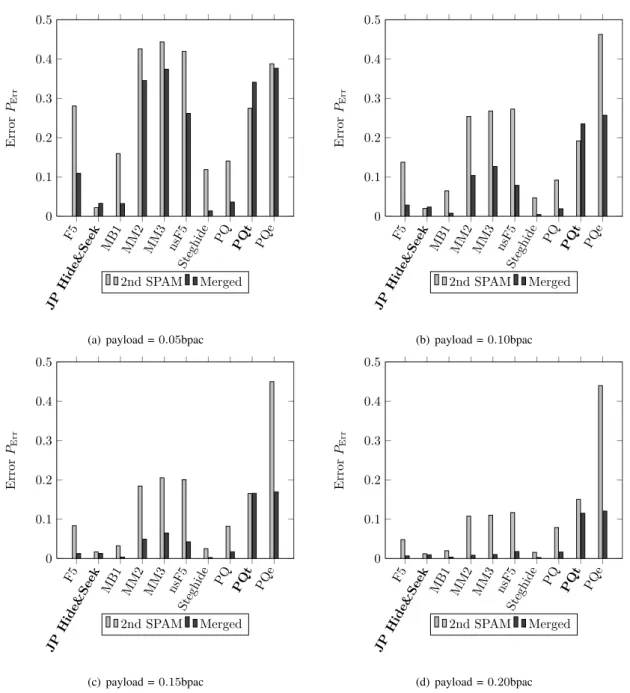
The database used for the comparison contained approximately 6000 single-compressed JPEG images with quality factor 70 and sizes ranging from 1.5 to 6Mpix, embedded by the following ten popular steganographic algorithms for JPEG images: F5 [39], F5 with shrinkage removed by wet paper codes [24] (nsF5), Model Based Steganography without deblocking (MB1) [32], JP Hide&Seek [2], MMx [21], Steghide [12], and perturbed quantization [9] (PQ) and its variants PQe and PQt [24] with payloads 5%, 10%, 15%, and 20% of bits per non-zero AC coefficient (bpac). The total number of images in the database was 4 ×11×6000 = 264, 000. The quality factor of JPEG images was fixed because steganalyzers employing Merged features, which are used as a reference, are sensitive to the mismatch between quality factors of the training and testing images. In fact, as reported in [30], JPEG images should be steganalyzed by classifiers separately designed for each quality factor. For each steganographic algorithm and payload, a steganalyzer embodied by an SVM with a Gaussian kernel (total number of steganalyzers was 2 × 10 × 4 = 80) was created using the procedure described in Section III. For ease of comparison, the error rates PErr of steganalyzers estimated from the testing set are displayed in

Figure 5. Generally, the accuracy of steganalyzers using the SPAM features is inferior to steganalyzers that use the Merged features, but still their performance is far from random guessing except for small payloads of 5% and the PQe algorithm. Surprisingly, for small payloads of 5% and 10%, the SPAM features are better in detecting JP Hide&Seek and the variation of perturbed quantization PQt.

B. Detecting YASS

YASS steganography for JPEG images published in [35] and further improved in [33] was developed to evade calibration-based steganalysis. Indeed, the accuracy of steganalysis with Merged features, where the calibration plays the central role, is very poor. Kodovský et al. [22] showed that YASS is more detectable using an uncalibrated version of Merged features. Since YASS significantly distorts the image due to repeated JPEG compression and robust embedding, it makes sense to use SPAM features to detect this distortion.

Although it would be valuable to compare the error rates of detection of YASS on the same payloads as in the previous subsection, the implementation of the algorithm (kindly provided by authors of [33]) does not allow setting an exact payload or hide a particular message. The implementation always hides the maximum embeddable message whose length significantly varies with image content and is also a function of the hiding block size, the hiding and the advertising quality factors, and the error correction phase. The embedding rates

F5 JP Hide &Se ek MB 1 MM2 MM3 nsF5 Stegh ide _{PQ PQt PQe} 0 0.1 0.2 0.3 0.4 0.5 E rr or PEr r 2nd SPAM Merged

(a) payload = 0.05bpac

F5 JP Hide &Se ek MB 1 MM2 MM3 nsF5 Stegh ide _{PQ PQt PQe} 0 0.1 0.2 0.3 0.4 0.5 E rr or PEr r 2nd SPAM Merged (b) payload = 0.10bpac F5 JP Hide &Se ek MB 1 MM2 MM3 nsF5 Stegh ide _{PQ PQt PQe} 0 0.1 0.2 0.3 0.4 0.5 E rr or PEr r 2nd SPAM Merged (c) payload = 0.15bpac F5 JP Hide &Se ek MB 1 MM2 MM3 nsF5 Stegh ide _{PQ PQt PQe} 0 0.1 0.2 0.3 0.4 0.5 E rr or PEr r 2nd SPAM Merged (d) payload = 0.20bpac

Figure 5. Error rates PErrof steganalyzers employing the second-order SPAM features with T = 3 and the Merged features.

shown in Table VII are average payloads over the corpus of the images. This is why we have estimated the detectability of five different YASS settings (see Appendix A for the settings) on 6500 JPEG images using the second-order SPAM features with T = 3, calibrated, and uncalibrated Merged features. Since the implementation of YASS is rather slow, we resized all images in the database so that their smaller side was 512 pixels. Note that this is exactly the same database that was used in [23].

As in all previous sections, we divided all images evenly into the training and testing set and created 3 × 5 SVM-based steganalyzers following the methodology described in Section III. The errors PErrare summarized in

Table VII. We can see that steganalyzers based on the second-order SPAM features are superior to steganalyzers based on the Merged feature set and its uncalibrated version. The important aspect of the presented attack is that it is blind in the sense that it is not based on any implementation shortcoming of the specific implementation

YASS setting 1 2 3 4 5 Cal. Merged 0.324 0.348 0.133 0.300 0.229 Non-cal. Merged 0.170 0.200 0.134 0.152 0.095 2nd_{SPAM 0.130 0.151 0.111 0.134 0.094}

Table VII

ERRORSPErrOF STEGANALYZERS EMPLOYING THE CALIBRATEDMERGED(CAL. MERGED),NON-CALIBRATEDMERGED(NON-CAL.

MERGED),AND THE SECOND-ORDERSPAMFEATURES ONYASSSTEGANOGRAPHY. THE ERRORS ARE CALCULATED ON THE

TESTING SET.

of YASS, unlike the targeted attack reported in [25].

VI. CONCLUSION

Majority of steganographic methods can be interpreted as adding independent realizations of stego noise to the cover digital media object. This paper presents a novel approach to steganalysis of such embedding methods by utilizing the fact that the noise component of typical digital media exhibits short-range dependences while the stego noise is an independent random component typically not found in digital media. The local dependences between differences of neighboring cover elements are modeled as a Markov chain, whose empirical probability transition matrix is taken as a feature vector for steganalysis.

The accuracy of the presented feature sets was carefully examined by using four different databases of images. The inter- and intra-database errors were estimated and the feature set was compared to prior art. It was also shown that even though the presented feature set was developed primarily to attack spatial domain steganography, it reliably detects algorithms hiding in the block DCT domain as well.

In the future, we would like to investigate the accuracy of regression-based quantitative steganalyzers [31] of LSB matching with second-order SPAM features. We also plan to investigate third-order Markov chain features, where the major challenge would be dealing with high feature dimensionality.

REFERENCES [1] http://photogallery.nrcs.usda.gov/.

[2] JP Hide & Seek. http://linux01.gwdg.de/~alatham/stego.html.

[3] P. Bas and T. Furon. BOWS-2. http://bows2.gipsa-lab.inpg.fr, July 2007.

[4] G. Cancelli, G. Doërr, I. Cox, and M. Barni. A comparative study of ±1 steganalyzers. In Proceedings IEEE, International Workshop on Multimedia Signal Processing, pages 791–794, Queensland, Australia, October 2008.

[5] G. Cancelli, G. Doërr, I. Cox, and M. Barni. Detection of ±1 steganography based on the amplitude of histogram local extrema. In Proceedings IEEE, International Conference on Image Processing,ICIP, San Diego, California, October 12–15, 2008.

[6] H. Farid and L. Siwei. Detecting hidden messages using higher-order statistics and support vector machines. In F. A. P. Petitcolas, editor, Information Hiding, 5th International Workshop, volume 2578 of Lecture Notes in Computer Science, pages 340–354, Noordwijkerhout, The Netherlands, October 7–9, 2002. Springer-Verlag, New York.

[7] J. Fridrich. Feature-based steganalysis for JPEG images and its implications for future design of steganographic schemes. In J. Fridrich, editor, Information Hiding, 6th International Workshop, volume 3200 of Lecture Notes in Computer Science, pages 67–81, Toronto, Canada, May 23–25, 2004. Springer-Verlag, New York.

[8] J. Fridrich and M. Goljan. Digital image steganography using stochastic modulation. In E. J. Delp and P. W. Wong, editors, Proceedings SPIE, Electronic Imaging, Security and Watermarking of Multimedia Contents V, volume 5020, pages 191–202, Santa Clara, CA, January 21–24, 2003.

[9] J. Fridrich, M. Goljan, and D. Soukal. Perturbed quantization steganography using wet paper codes. In J. Dittmann and J. Fridrich, editors, Proceedings of the 6th ACM Multimedia & Security Workshop, pages 4–15, Magdeburg, Germany, September 20–21, 2004. [10] M. Goljan, J. Fridrich, and T. Holotyak. New blind steganalysis and its implications. In E. J. Delp and P. W. Wong, editors, Proceedings SPIE, Electronic Imaging, Security, Steganography, and Watermarking of Multimedia Contents VIII, volume 6072, pages 1–13, San Jose, CA, January 16–19, 2006.

[11] J. J. Harmsen and W. A. Pearlman. Steganalysis of additive noise modelable information hiding. In E. J. Delp and P. W. Wong, editors, Proceedings SPIE, Electronic Imaging, Security and Watermarking of Multimedia Contents V, volume 5020, pages 131–142, Santa Clara, CA, January 21–24, 2003.

[12] S. Hetzl and P. Mutzel. A graph–theoretic approach to steganography. In J. Dittmann, S. Katzenbeisser, and A. Uhl, editors, Communications and Multimedia Security, 9th IFIP TC-6 TC-11 International Conference, CMS 2005, volume 3677 of Lecture Notes in Computer Science, pages 119–128, Salzburg, Austria, September 19–21, 2005.

[13] T. S. Holotyak, J. Fridrich, and S. Voloshynovskiy. Blind statistical steganalysis of additive steganography using wavelet higher order statistics. In J. Dittmann, S. Katzenbeisser, and A. Uhl, editors, Communications and Multimedia Security, 9th IFIP TC-6 TC-11 International Conference, CMS 2005, Salzburg, Austria, September 19–21, 2005.

[14] C. Hsu, C. Chang, and C. Lin. A Practical Guide to ± Support Vector Classification. Department of Computer Science and Information Engineering, National Taiwan University, Taiwan.

[15] J. Huang and D. Mumford. Statistics of natural images and models. In Proceedngs of IEEE Conference on Computer Vision and Pattern Recognition, volume 1, page 547, 1999.

[16] A. D. Ker. A general framework for structural analysis of LSB replacement. In M. Barni, J. Herrera, S. Katzenbeisser, and F. Pérez-González, editors, Information Hiding, 7th International Workshop, volume 3727 of Lecture Notes in Computer Science, pages 296–311, Barcelona, Spain, June 6–8, 2005. Springer-Verlag, Berlin.

[17] A. D. Ker. Steganalysis of LSB matching in grayscale images. IEEE Signal Processing Letters, 12(6):441–444, June 2005. [18] A. D. Ker. A fusion of maximal likelihood and structural steganalysis. In T. Furon, F. Cayre, G. Doërr, and P. Bas, editors, Information

Hiding, 9th International Workshop, volume 4567 of Lecture Notes in Computer Science, pages 204–219, Saint Malo, France, June 11–13, 2007. Springer-Verlag, Berlin.

[19] A. D. Ker and R. Böhme. Revisiting weighted stego-image steganalysis. In E. J. Delp and P. W. Wong, editors, Proceedings SPIE, Electronic Imaging, Security, Forensics, Steganography, and Watermarking of Multimedia Contents X, volume 6819, pages 5 1–5 17, San Jose, CA, January 27–31, 2008.

[20] A. D. Ker and I. Lubenko. Feature reduction and payload location with WAM steganalysis. In E. J. Delp and P. W. Wong, editors, Proceedings SPIE, Electronic Imaging, Media Forensics and Security XI, volume 6072, pages 0A01–0A13, San Jose, CA, January 19–21, 2009.

[21] Y. Kim, Z. Duric, and D. Richards. Modified matrix encoding technique for minimal distortion steganography. In J. L. Camenisch, C. S. Collberg, N. F. Johnson, and P. Sallee, editors, Information Hiding, 8th International Workshop, volume 4437 of Lecture Notes in Computer Science, pages 314–327, Alexandria, VA, July 10–12, 2006. Springer-Verlag, New York.

[22] J. Kodovský and J. Fridrich. Influence of embedding strategies on security of steganographic methods in the JPEG domain. In E. J. Delp and P. W. Wong, editors, Proceedings SPIE, Electronic Imaging, Security, Forensics, Steganography, and Watermarking of Multimedia Contents X, volume 6819, pages 2 1–2 13, San Jose, CA, January 27–31, 2008.

[23] J. Kodovský and J. Fridrich. Calibration revisited. In Proceedings of the 11th ACM Multimedia & Security Workshop, Princeton, NJ, September 7–8, 2009.

[24] J. Kodovský, J. Fridrich, and T. Pevný. Statistically undetectable JPEG steganography: Dead ends, challenges, and opportunities. In J. Dittmann and J. Fridrich, editors, Proceedings of the 9th ACM Multimedia & Security Workshop, pages 3–14, Dallas, TX, September 20–21, 2007.

[25] B. Li, J. Huang, and Y. Q. Shi. Steganalysis of yass. In A. D. Ker, J. Dittmann, and J. Fridrich, editors, Proceedings of the 10th ACM Multimedia & Security Workshop, pages 139–148, Oxford, UK, 2008.

[26] X. Li, T. Zeng, and B. Yang. Detecting LSB matching by applying calibration technique for difference image. In A. D. Ker, J. Dittmann, and J. Fridrich, editors, Proceedings of the 10th ACM Multimedia & Security Workshop, pages 133–138, Oxford, UK, September 22–23, 2008.

[27] M. K. Mihcak, I. Kozintsev, K. Ramchandran, and P. Moulin. Low-complexity image denoising based on statistical modeling of wavelet coefficients. IEEE Signal Processing Letters, 6(12):300–303, December 1999.

[28] T. Pevný, P. Bas, and J. Fridrich. Steganalysis by subtractive pixel adjacency matrix. In Proceedings of the 11th ACM Multimedia & Security Workshop, pages 75–84, Princeton, NJ, September 7–8, 2009.

[29] T. Pevný and J. Fridrich. Merging Markov and DCT features for multi-class JPEG steganalysis. In E. J. Delp and P. W. Wong, editors, Proceedings SPIE, Electronic Imaging, Security, Steganography, and Watermarking of Multimedia Contents IX, volume 6505, pages 3 1–3 14, San Jose, CA, January 29 – February 1, 2007.

[30] T. Pevný and J. Fridrich. Multiclass detector of current steganographic methods for JPEG format. IEEE Transactions on Information Forensics and Security, 3(4):635–650, December 2008.

[31] T. Pevný, J. Fridrich, and A. D. Ker. From blind to quantitative steganalysis. In N. D. Memon, E. J. Delp, P. W. Wong, and J. Dittmann, editors, Proceedings SPIE, Electronic Imaging, Security and Forensics of Multimedia XI, volume 7254, pages 0C 1–0C 14, San Jose, CA, January 18–21, 2009.

[32] P. Sallee. Model-based steganography. In T. Kalker, I. J. Cox, and Y. Man Ro, editors, Digital Watermarking, 2nd International Workshop, volume 2939 of Lecture Notes in Computer Science, pages 154–167, Seoul, Korea, October 20–22, 2003. Springer-Verlag, New York.

[33] A. Sarkar, K. Solanki, and B. S. Manjunath. Further study on YASS: Steganography based on randomized embedding to resist blind steganalysis. In E. J. Delp and P. W. Wong, editors, Proceedings SPIE, Electronic Imaging, Security, Forensics, Steganography, and Watermarking of Multimedia Contents X, volume 6819, pages 16–31, San Jose, CA, January 27–31, 2008.

[34] Y. Q. Shi, C. Chen, and W. Chen. A Markov process based approach to effective attacking JPEG steganography. In J. L. Camenisch, C. S. Collberg, N. F. Johnson, and P. Sallee, editors, Information Hiding, 8th International Workshop, volume 4437 of Lecture Notes in Computer Science, pages 249–264, Alexandria, VA, July 10–12, 2006. Springer-Verlag, New York.

[35] K. Solanki, A. Sarkar, and B. S. Manjunath. YASS: Yet another steganographic scheme that resists blind steganalysis. In T. Furon, F. Cayre, G. Doërr, and P. Bas, editors, Information Hiding, 9th International Workshop, volume 4567 of Lecture Notes in Computer Science, pages 16–31, Saint Malo, France, June 11–13, 2007. Springer-Verlag, New York.

[36] D. Soukal, J. Fridrich, and M. Goljan. Maximum likelihood estimation of secret message length embedded using ±k steganography in spatial domain. In E. J. Delp and P. W. Wong, editors, Proceedings SPIE, Electronic Imaging, Security, Steganography, and Watermarking of Multimedia Contents VII, volume 5681, pages 595–606, San Jose, CA, January 16–20, 2005.

[37] K. Sullivan, U. Madhow, S. Chandrasekaran, and B.S. Manjunath. Steganalysis of spread spectrum data hiding exploiting cover memory. In E. J. Delp and P. W. Wong, editors, Proceedings SPIE, Electronic Imaging, Security, Steganography, and Watermarking of Multimedia Contents VII, volume 5681, pages 38–46, San Jose, CA, January 16–20, 2005.

[38] V. N. Vapnik. The Nature of Statistical Learning Theory. Springer-Verlag, New York, 1995.

[39] A. Westfeld. High capacity despite better steganalysis (F5 – a steganographic algorithm). In I. S. Moskowitz, editor, Information Hiding, 4th International Workshop, volume 2137 of Lecture Notes in Computer Science, pages 289–302, Pittsburgh, PA, April 25–27, 2001. Springer-Verlag, New York.

[40] G. Xuan, Y. Q. Shi, J. Gao, D. Zou, C. Yang, Z. Z. P. Chai, C. Chen, and W. Chen. Steganalysis based on multiple features formed by statistical moments of wavelet characteristic functions. In M. Barni, J. Herrera, S. Katzenbeisser, and F. Pérez-González, editors, Information Hiding, 7th International Workshop, volume 3727 of Lecture Notes in Computer Science, pages 262–277, Barcelona, Spain, June 6–8, 2005. Springer-Verlag, Berlin.

[41] D. Zo, Y. Q. Shi, W. Su, and G. Xuan. Steganalysis based on Markov model of thresholded prediction-error image. In Proc. of IEEE International Conference on Multimedia and Expo, pages 1365–1368, Toronto, Canada, July 9-12, 2006.

APPENDIX

We use five different configurations for YASS, including both the original version of the algorithm published in [35] as well as its modifications [33]. Using the same notation as in the corresponding original publications, QFhis the hiding quality factor(s) and B is the big block size. Settings 1, 4, and 5 incorporate a mixture-based

modification of YASS embedding with several different values of QFhbased on block variances (the decision

boundaries are in the column “DBs”). Setting 3 uses attack-aware iterative embedding (column rep). Since the implementation of YASS we used in our tests, did not allow direct control over the real payload size, we were repetitively embedding in order to find minimal payload that would be reconstructed without errors. Payload values obtained this way are listed in Table VIII in terms of bits per non-zero AC DCT coefficient (bpac), averaged over all images in our database. In all experiments, the advertising quality factor was fixed at

QFa= 75 and the input images were in the raw (uncompressed) format. With these choices, YASS appears to

be the least detectable [22].

Awerage Notation QFh DBs B rep payload

YASS 1 65,70,75 3,7 9 0 0.110 YASS 2 75 - 9 0 0.051 YASS 3 75 - 9 1 0.187 YASS 4 65,70,75 2,5 9 0 0.118 YASS 5 50,55,60,65,70 3,7,12,17 9 0 0.159 Table VIII