Climate model uncertainty in impact assessments for agriculture: A multi-ensemble case study on maize in sub-Saharan Africa

The MIT Faculty has made this article openly available.

Please share

how this access benefits you. Your story matters.

Citation

Dale, Amy, Charles Fant, Kenneth Strzepek, Megan Lickley, and

Susan Solomon. “Climate Model Uncertainty in Impact Assessments

for Agriculture: A Multi-Ensemble Case Study on Maize in

Sub-Saharan Africa.” Earth’s Future 5, no. 3 (March 2017): 337–353.

As Published

http://dx.doi.org/10.1002/2017EF000539

Publisher

Wiley Blackwell

Version

Final published version

Citable link

http://hdl.handle.net/1721.1/109497

Terms of Use

Creative Commons Attribution-NonCommercial-NoDerivs License

agriculture: A multi-ensemble case study on maize in

sub-Saharan Africa

Amy Dale1,2_{, Charles Fant}1_{, Kenneth Strzepek}1_{, Megan Lickley}2_{, and Susan Solomon}1,2

1_{Joint Program on the Science and Policy of Global Change, Massachusetts Institute of Technology, Cambridge,} Massachusetts, USA,2_{Department of Earth, Atmospheric and Planetary Sciences, Massachusetts Institute of} Technology, Cambridge, Massachusetts, USA

Abstract

We present maize production in sub-Saharan Africa as a case study in the exploration of how uncertainties in global climate change, as reflected in projections from a range of climate model ensem-bles, influence climate impact assessments for agriculture. The crop model AquaCrop-OS (Food and Agri-culture Organization of the United Nations) was modified to run on a 2∘ × 2∘ grid and coupled to 122 cli-mate model projections from multi-model ensembles for three emission scenarios (Coupled Model Inter-comparison Project Phase 3 [CMIP3] SRES A1B and CMIP5 Representative Concentration Pathway [RCP] scenarios 4.5 and 8.5) as well as two “within-model” ensembles (NCAR CCSM3 and ECHAM5/MPI-OM) designed to capture internal variability (i.e., uncertainty due to chaos in the climate system). In spite of high uncertainty, most notably in the high-producing semi-arid zones, we observed robust regional and sub-regional trends across all ensembles. In agreement with previous work, we project widespread yield losses in the Sahel region and Southern Africa, resilience in Central Africa, and sub-regional increases in East Africa and at the southern tip of the continent. Spatial patterns of yield losses corresponded with spa-tial patterns of aridity increases, which were explicitly evaluated. Internal variability was a major source of uncertainty in both within-model and between-model ensembles and explained the majority of the spatial distribution of uncertainty in yield projections. Projected climate change impacts on maize pro-duction in different regions and nations ranged from near-zero or positive (upper quartile estimates) to substantially negative (lower quartile estimates), highlighting a need for risk management strategies that are adaptive and robust to uncertainty.

1. Introduction

Uncertainty in projections of the socioeconomic, ecological, and health impacts of climate change has become a major topic of study in the last decade. Early impact studies relied on output from single general circulation model (GCM) runs; this is no longer an accepted method, and most authors now use multiple GCMs to generate a range of possible climate futures, thereby limiting the influence of errors in any one model [Tebaldi and Knutti, 2007; Hawkins and Sutton, 2011].

Multi-model GCM ensembles are necessary for the detailed exploration of uncertainty in climate model projections, but they are not necessarily sufficient. Often, each member of an ensemble is represented by a single model run, or one possible realization of a system whose behavior—due to the chaotic nature of the climate system—is highly sensitive to small perturbations of initial conditions. Thus, multi-model ensembles confound the large uncertainties that arise from sources of internal variability such as El Niño with structural uncertainties related to between-model differences in model structure, parameter selection, and boundary conditions (“model uncertainty”) [Tebaldi and Knutti, 2007]. The choice of greenhouse gas emission scenario also gives rise to “scenario uncertainty.”

The relative influence of each source of uncertainty varies with time; the influence of scenario uncertainty increases over time, whereas the influence of internal variability and model uncertainty decreases [Hawkins

and Sutton, 2011]. Deser et al. [2012] attribute at least half of all uncertainty in the Coupled Model

Intercom-parison Project Phase 3 (CMIP3) multi-model ensemble from 2005 to 2060 to internal variability. At regional scales (∼2,500 km), Hawkins and Sutton [2011] found that internal variability in projections of decadal mean

10.1002/2017EF000539

Key Points:

• We estimate the influence of global climate model uncertainty on projected maize yield changes in sub-Saharan Africa due to climate change

• Five different GCM ensembles all project yield losses in the Sahel region and Southern Africa and sub-regional increases in East Africa • Irreducible internal variability is a

major cause of uncertainty in crop model projections even out to 2090

Supporting Information: • Supporting Information S1 • Data Set S1 Corresponding author: A. Dale, amydale@mit.edu Citation:

Dale, A., C. Fant, K. Strzepek, M. Lickley, and S. Solomon (2017), Climate model uncertainty in impact assessments for agriculture: A multi-ensemble case study on maize in sub-Saharan Africa,

Earth’s Future, 5, 337–353,

doi:10.1002/2017EF000539.

Received 15 JAN 2017 Accepted 28 FEB 2017

Accepted article online 15 MAR 2017 Published online 22 MAR 2017

© 2017 The Authors.

This is an open access article under the terms of the Creative Commons Attribution-NonCommercial-NoDerivs License, which permits use and distri-bution in any medium, provided the original work is properly cited, the use is non-commercial and no modifica-tions or adaptamodifica-tions are made.

precipitation changes was comparable in magnitude to scenario uncertainty, even when the latter was at 2100 levels.

“Within-model” ensembles are comprised of multiple runs of a single GCM that differ only with respect to small variations in the initial conditions. Because within-model ensembles are subject only to internal vari-ability, comparisons of “within-” and “between-model” ensembles shed important light on the magnitude of internal variability and its relative influence. Such comparisons have practical relevance in the develop-ment of appropriate adaptation and mitigation strategies: they separate the sources of uncertainty that are theoretically reducible (model and scenario uncertainty) from those that largely are not (internal variability) [Hawkins and Sutton, 2009].

Boehlert et al. [2015] used multiple within- and between-model GCM ensembles to assess the impact of

cli-mate model uncertainties on projected changes in runoff, crop water requirements, and adaptation costs out to 2090. Our work extends the multi-ensemble approach of Boehlert et al. [2015] to the problem of cli-mate change impacts on maize production in sub-Saharan Africa (SSA).

Nations in SSA are expected to experience substantial future changes in agricultural production due to cli-mate change [Niang et al., 2014] and have relatively limited capital and institutional capacity to address the potential threat [Challinor et al., 2007; Knox et al., 2012]. Almost a quarter of the world’s malnourished pop-ulation lives in SSA [Lobell et al., 2008], yet, agriculture in this region comprises up to 50% of gross domestic product (GDP) in some countries [Schlenker and Lobell, 2010]. Maize is the most widely produced crop in SSA by harvested area [Food and Agriculture Organization of the United Nations, 2015] and is also the most calor-ically important [Schlenker and Lobell, 2010]. As a drought-sensitive species, it is also one of the crops that is most likely to be negatively impacted by climate change [Schlenker and Lobell, 2010; Rippke et al., 2016]. This is especially true in SSA, where the vast majority of cereal crop production relies on rainfall rather than irri-gation [Challinor et al., 2007]. A systematic review of over 50 studies on climate change impacts on African crop yields from the field to regional scales revealed that the projected maize impacts of climate change display large uncertainties, with projected future changes ranging from nearly −50 to +100% [Knox et al., 2012].

Previous studies on maize production under climate change either globally or in SSA have relied on a single GCM or on limited multi-model ensembles [Lobell et al., 2008; Schlenker and Lobell, 2010; Thornton et al., 2011; Knox et al., 2012; Waha et al., 2013; Rosenzweig et al., 2014; Rippke et al., 2016]. A much richer range of within and between-model climate model ensembles has become available since these studies, and a deeper elucidation of uncertainty using this information is the primary focus and motivation for this paper. We present results for a recently released open-source process-based crop model (FAO AquaCrop-OS v5.0a) coupled to projections from 122 GCM runs representing three between-model ensembles, two within-model ensembles, three emission scenarios, and both CMIP3 and CMIP5. This approach allowed us to identify regions in which the potential risks (and benefits) to the food supply due to climate change are robust across and within ensembles, as well as regions in which disagreement persists. It allowed us to evaluate the potential benefits of greenhouse gas mitigation, separate the influence of internal variability from that of model uncertainty and scenario uncertainty, and attribute regional shifts in crop production (and their associated uncertainties) to underlying shifts (and uncertainties) in temperature, precipitation, and aridity. We conclude with a comparison of our projections to projections from previous works and a discussion of their implications for the development of more robust impact assessments and management strategies.

2. Data and Methods

2.1. Climate Data and Processing

We used five ensembles from the World Climate Research Programme’s (WCRP’s) CMIP phase 3 (CMIP3) and phase 5 (CMIP5) multi-model dataset [Meehl et al., 2007; Taylor et al., 2012]. The three CMIP3 ensem-bles, which were run with the Special Report on Emissions Scenarios (SRES) A1B scenario, included a between-model ensemble of 22 projections from different GCMs and two within-model ensembles, 17 projections for the European Centre Hamburg Model Version 5/Max Planck Institute-Ocean Model (ECHAM5/MIP-OM) model [Sterl et al., 2008] and 40 projections for the National Center for Atmospheric Research Community Climate System Model Version 3 (NCAR CCSM3) [Deser et al., 2012]. The two CMIP5

ensembles included 23 projections for the Representative Concentration Pathway (RCP) 4.5 scenario (a mid-range emissions scenario) and 20 projections for RCP8.5 (high emissions scenario). The names of the specific CMIP3 and CMIP5 models used in this study are presented in Tables S1 and S2, Supporting Information [also presented in Boehlert et al., 2015]. GCM projections were regridded from their native resolution to the common 2∘ × 2∘ resolution as described by Boehlert [2015].

We consider four eras: “2010,” “2030,” “2050,” and “2090.” Each era represents an average over 20 years of projected changes in temperature and precipitation. For example, “2010” represents 2000–2019 and “2050” represents 2040–2059. Results are not available for the NCAR within-model ensemble beyond 2060. In order to correct the biases in the GCMs, we applied the simple change factor method presented by

Hawkins et al. [2013] (the “delta” method) to historical data from Princeton’s global meteorological

forc-ing dataset [Sheffield et al., 2006]. This method is common in climate change impact studies [Arndt et al., 2011; Boehlert et al., 2015; Fant et al., 2016]. In this approach, we “nudge” historical daily climate data over the period 1961–1990 by changes in the mean temperature and precipitation projected for a given era by the GCMs. For example, for the 2050 era, the mean change in temperature (the “delta”) was taken to be the monthly mean temperature difference between GCM projections from 2040 to 2059 and the monthly mean from 1961 to 1990. This “delta” was then added to the daily historical climate data for the same base-line period, 1961–1990. In order to maintain the daily precipitation pattern, we applied the same method as for temperature but apportioned the monthly mean change in precipitation on a given day according to the fraction of the total monthly historical precipitation that occurred on that day. The crop yield reported below for each era is the average annual yield over a 30-year simulation (preceded by 5 years of model “spin up”) driven by the 1961–1990 climate nudged by computed changes in temperature and precipitation. A possible shortcoming of the delta method is that it cannot address changes in climate variability over time. However, this assumption may be preferable in light of the ongoing uncertainties regarding the ability of GCMs to reliably project future changes in climate variability [Blöschl et al., 2007; Brown and Wilby, 2012]. 2.2. Crop Model

AquaCrop (Food and Agriculture Organization of the United Nations) is a one-dimensional (“point”) model designed for use at the field scale. It performs well for maize under a wide range of environmental conditions and nutrient management scenarios [Heng et al., 2009; Hsiao et al., 2009; Steduto et al., 2011; Abedinpour

et al., 2012; Kim and Kaluarachchi, 2015; Greaves and Wang, 2016], although its performance can suffer under

severe water stress [Hsiao et al., 2009; Ahmadi et al., 2015; Greaves and Wang, 2016]. Despite its comparatively simple structure and limited input requirements, its performance was also comparable to, or superior to, that of other crop models in three cross-model comparisons for sunflower, barley, winter wheat, and maize [Todorovic et al., 2009; Eitzinger et al., 2013; Saab et al., 2015].

We refer readers to the AquaCrop manual for a detailed description of its formulation and data require-ments [Raes et al., 2012]. Briefly, AquaCrop models the daily climate-driven soil water balance as well as crop growth, transpiration, and senescence in the presence or absence of management scenarios such as irrigation and fertilization. Five “water stress coefficients” are varied daily from 1 (no stress) to 0 (maximum stress) in order to modify crop-specific parameters that determine the rates of canopy expansion, transpira-tion, senescence, and root growth as well as the harvest index (HI, or the fraction of the total above-ground biomass that results in yield). Biomass and yield are calculated as follows:

B = KsbWP ∗∑ d Trd ET0d (1) Y = HI · B (2)

where B is the total above-ground dry biomass over the entire growing season, Ksbis a temperature stress coefficient, WP* is the crop water productivity (i.e., the crop’s ability to convert water consumed/transpired into biomass) normalized by the daily reference evapotranspiration and atmospheric CO2, Trdis the crop transpiration on day d; ET0dis the reference evapotranspiration on day d; and Y is the crop yield. Normal-ization of WP* by ET0dand CO2ensures that AquaCrop is applicable under a wide range of atmospheric conditions. As is suggested by the appearance of Ksbin the biomass formula, AquaCrop considers several

sources of stress in addition to water: heat stress, cold stress, soil infertility, and (not included in our work) soil salinity.

We used the Modified Hargreaves method adjusted for a daily timestep to estimate ET0d[Farmer et al., 2011]. Droogers and Allen [2002] showed that Modified Hargreaves is likely to outperform the more standard and

substantially more data-intensive Penman–Monteith method [Allen et al., 1998] when meteorological data are uncertain or error-prone, as is commonly the case for weather stations in SSA [Vrieling et al., 2013]. We modified FAO’s recently released open-source MATLAB version of AquaCrop (AquaCrop-OS v5.0a) to run for all grid cells in SSA at 2o_{× 2∘ resolution [Foster, 2016]. The conversion of site-scale crop models to} gridded crop models in this manner is a common practice [Rosenzweig et al., 2014]. The supporting methods (including Figures S1–S6) provide details on model setup, calibration, and benchmarking procedures and results. Key model features are summarized here.

We modeled two soil layers with different hydraulic properties (topsoil and subsoil) using 18 soil compart-ments that expanded in thickness from 1 cm at the surface to 30 cm at depth. Pedotransfer functions [U.S.

Department of the Interior, Bureau of Reclamation, 1993; Nemes et al., 2005; Mohamed and Ali, 2006] were used

to estimate the hydraulic properties in each grid cell from the subsoil and topsoil composition reported in the Regridded Harmonized World Soil Database v1.2 [Wieder et al., 2014]. To ensure accurate initial condi-tions, we modeled the soil water balance for 5 years before collecting model results (“spin-up”). We did not model groundwater table effects on water logging and capillary rise [Fan et al., 2013].

In addition to climate-driven (rain-fed) crop growth, we accounted for the influence of fertilizer application [Stoorvogel et al., 1993; Sanchez, 2002] and irrigation [Frenken, 2005] on crop yields. However, fertilizer use, irrigation, and the maize harvested area were held constant over all eras in order to explore climate change impacts in the absence of land use change. Estimates of the harvested area in each grid cell and nitro-gen, phosphorus, and potash fertilizer application rates for maize were downloaded from EarthStat (www .earthstat.org) [Monfreda et al., 2008; Mueller et al., 2012]. The ability of fertilizer to improve crop yields was captured as part of a multi-step calibration procedure based on AquaCrop’s soil fertility stress equations. The crop yields reported in the results are the weighted results for a “no irrigation” and “complete irriga-tion” scenario, where the weighting factor is the fraction of the harvested maize area in each grid cell that was equipped for irrigation [Frenken, 2005; Siebert et al., 2005; Siebert et al., 2013]. Raw fertilizer and irrigation data were upscaled from 0.05∘ × 0.05∘ to 2∘ × 2∘ as needed by taking the weighted average with respect to the fraction of the harvested maize area represented by each subcell.

We used a simplified version of the temperature and precipitation rules proposed by Waha et al. [2012] to optimize planting dates in each grid cell based on the climate for the current year. As a result, our projections may be more conservative than those of models that do not allow planting dates to adapt to climate change (e.g., four out of seven of the Agricultural Model Intercomparison and Improvement Project [AgMIP] models [Rosenzweig et al., 2014]).

We did not account for improved yields due to CO2enrichment. However, CO2effects are thought to be smaller for C4crops such as maize than they are for C3crops [Schlenker and Lobell, 2010]. Interestingly, two meta-analyses found no significant difference in projected crop yield responses to climate change between C3and C4crops, suggesting a potentially limited role for CO2effects in the face of other cross-study differ-ences [Knox et al., 2012; Challinor et al., 2014].

We calibrated (“tuned”) the model by minimizing the root mean squared error between national yields reported by FAOSTAT for the year 2000 [Food and Agriculture Organization of the United Nations, 2015] and the 7-year average yields produced by the model when driven by historical Princeton climate data from 1997 to 2003. After calibration, we compared AquaCrop’s performance against that of three gridded crop models from the AgMIP Fast Track project (LPJmL, PEGASUS, and pDSSAT [Deryng et al., 2011; Rosenzweig

et al., 2014]) with respect to both the FAOSTAT data and aggregated sub-national estimates from FAO [2016], Fischer et al. [2012], and Mueller et al. [2012] (Figures S5–S6). At 2∘ × 2∘ resolution, our model performed

notably better than PEGASUS and pDSSAT and marginally better than LPJmL. This is to be expected, since our calibration procedure was designed to minimize error in projections for SSA rather than the entire globe. We did not model any cell for which over 90% of the 0.05∘ × 0.05∘ subcells contained no harvest maize area [Monfreda et al., 2008]. Results are also not shown for any cell in which the simulation failed for over one

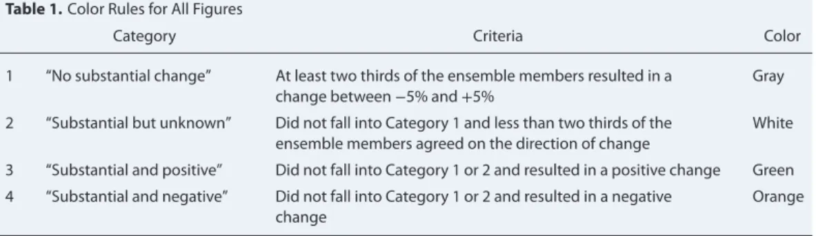
Table 1. Color Rules for All Figures

Category Criteria Color

1 “No substantial change” At least two thirds of the ensemble members resulted in a change between−5% and+5%

Gray

2 “Substantial but unknown” Did not fall into Category 1 and less than two thirds of the ensemble members agreed on the direction of change

White

3 “Substantial and positive” Did not fall into Category 1 or 2 and resulted in a positive change Green 4 “Substantial and negative” Did not fall into Category 1 or 2 and resulted in a negative

change

Orange

third of the ensemble members due to inadequate conditions for crop growth. These cells are shown in dark gray in all figures.

3. Results

We used AquaCrop to estimate the annual maize yield and production (yield × harvested area) in every grid cell in Africa for each ensemble member, ensemble, and era. The figures that follow use a common coloring scheme to describe median projected percent changes in yields and underlying climate drivers (Table 1): grid cells for which at least two thirds of the ensemble members resulted in a change between −5% and +5% were colored light gray, indicating cells for which projections of small or no changes were robust across GCM ensemble members. Cells that did not fall into the previous category, and for which less than two thirds of the ensemble members agreed on the direction of change, were colored white; these are areas in which a substantial change could occur, but there is disagreement regarding the direction of change. Cells that did not meet the criteria for the first two categories are cells in which a robust change was observed across ensemble members (i.e., greater than two thirds of the ensemble members agree on the direction of change and less than two thirds suggest a change within 5%); these cells were colored green or orange depending on whether the direction of change was positive or negative.

We present medians rather than means because yield and production estimates cannot fall below zero (or −100% change); thus, the distribution of projections for any given ensemble tends to be skewed, especially in cells that experienced large negative impacts. Note that the ensemble median in all maps (e.g., Figure 1) was calculated cell-by-cell and thus represents a composite scenario generated from all ensemble members, rather than results for a single representative ensemble.

3.1. Projected Climate Change

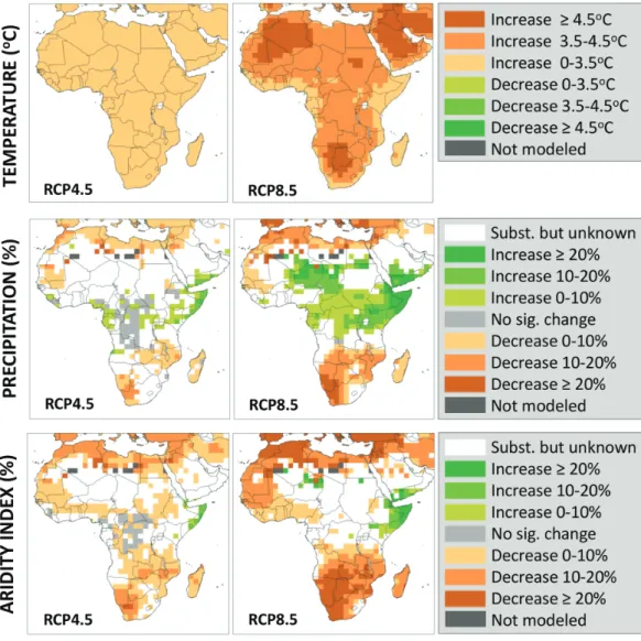
Figure 1 presents the median change in temperature, precipitation, and aridity index from 2010 to 2090 for the lowest and highest emission scenarios, CMIP5 RCP4.5 and RCP8.5. This figure lays the groundwork for a more detailed discussion of spatial variation in the projected maize yield response across all five ensembles (Section 3.2) and the relative influence of climate drivers on the yield response (Section 3.3).

The aridity index is a measure of the dryness of the terrestrial climate and was estimated as shown: AI =∑Pd∕

∑

ET0d (3)

where∑Pdis the total annual precipitation (summed over all days d) and ∑

ET0dis the total annual reference evapotranspiration [Middleton and Thomas, 1992; Fu and Feng, 2014]. Note that a positive percent change in AI implies decreasing aridity, or an increasingly wet climate.

As expected, both RCP4.5 and RCP8.5 project universally robust temperature increases, whereas within-ensemble disagreement regarding the direction of change in precipitation (white cells) is widespread, especially in RCP4.5. The RCP8.5 scenario projects robust increases in precipitation across much of the northern half of the continent and robust decreases south of the Democratic Republic of the Congo. Africa is projected to become more arid overall.

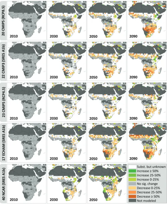
3.2. Projected Yield Change

Figure 2 shows the median percent change in crop yields between 2010 and all other eras for each of the ensembles.

Figure 1. Median absolute change in temperature (∘C) and percent change in precipitation and aridity index from 2010 to 2090 for

Coupled Model Intercomparison Project Phase 5 (CMIP5) Representative Concentration Pathway (RCP) scenarios 4.5 and 8.5. Note the inverted color scale for temperature. There were no white or gray cells in the temperature plot when expressed in terms of percent change (not shown).

Several spatial trends in the maize yield response to climate change were robust across ensembles in spite of cross-ensemble differences in the emission scenario, the model generation (CMIP3 vs. CMIP5), and the ensemble size and type (within- or between-model). All ensembles projected that robust negative effects (orange) will be more widespread than robust positive effects (green). Regionally, all projected the most widespread yield losses in the Sahel region and southern Africa below the Democratic Republic of the Congo and Tanzania. Sub-regionally, all projected yield increases in the Ethiopian highlands, at the southern tip of South Africa, and (tentatively, as many grid cells in this region produce little to no maize and were therefore not modeled) in the Horn of Africa. No ensemble projected a substantial median yield change within or surrounding the tropical rainforests of Central and West Africa. As expected, the crop yield response increased over time, and the fraction of cells characterized by “no substantial effect” or “substantial but unknown effects” (e.g., gray or white cells) decreased.

The magnitude of the crop yield responses reflects the emission scenario, such that 2090 results for the SRES A1B between-model ensemble were bounded by those of RCP4.5 (lower emissions, smaller response) and RCP8.5 (higher emissions, larger response). This trend was preserved across the CMIP3 and CMIP5 between-model ensembles, suggesting that the scenario ultimately had a larger influence on results than the choice of model generation.

Figure 2. Median percent change in maize yield for all ensembles from 2010 to 2010, 2030, 2050, and 2090. Results for the 40 NCAR runs

do not extend to 2090. The number in front of each ensemble name indicates the size of the ensemble. Color rules are described in Table 1.

The ECHAM5 ensemble was relatively pessimistic and the NCAR ensemble was relatively optimistic. As expected, both of these within-model ensembles showed lower within-ensemble disagreement (white) than the three between-model ensembles. In the ECHAM5 ensemble, white persisted to the greatest extent in Tanzania, Kenya, and Sudan; in the NCAR model, white persisted in the Sahel region and in Southern Africa. It is likely that internal variability is responsible for much of the disagreement in these regions across the multi-model CMIP3 ensemble.

Comparison of Figures 1 and 2 reveals general agreement between projected changes in crop yields and projected changes in AI over the next century: yields decreased in regions that are expected to become drier (e.g., Southern Africa, the western Sahel region); yields increased in the arid/semi-arid Horn of Africa,

which is projected to become more humid; yields and aridity index (AI) both changed least in the tropical rainforest, at least in the RCP4.5 scenario; and the spatial distribution of white (uncertain) regions is similar for both AI and yields. The relative insensitivity of AI to climate change in the tropical rainforest results from high precipitation in this region.

Overall, maize yield trends aligned more closely with trends in AI (a composite index that describes the com-bined effect of changes in temperature and precipitation) than with trends in temperature or precipitation alone (the raw inputs to AquaCrop), illustrating the potential value of aridity as an index for evaluating maize yield changes with climate. Further, it should be noted that increases in aridity imply that irrigation would become less effective in these regions for the same amount of water use.

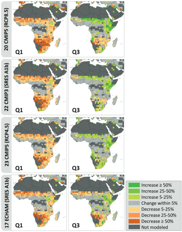
Figure 3 shows the 25th and 75th percentile (first and third quartile, or Q1 and Q3) percent change in maize yields from 2010 to 2090 in each grid cell across all ensemble members. The NCAR ensemble was not included because projections are not available for 2090. Each map represents an estimate of uncertainty based on these model runs, depicting a pessimistic and optimistic composite of future impacts under cli-mate change. Note that an analysis of the ensemble members associated with each median and quartile in Figure 3 (not shown) suggests that no single ensemble member dominated results in any region of any subplot.

Spatial trends that are robust (green and orange) in Figure 2 also appear here in both the Q1 and Q3 maps for each ensemble. Thus, the direction of the crop yield response in these regions is not only robust across two thirds of the ensemble members but is also robust within the interquartile range. The Q1 map shows regions of substantial crop losses (greater than 25%) near the subtropical Sahel edge region extending across a line of latitude spanning West, Central, and East Africa in all model ensembles, as well as in parts of Southern Africa. Even in the Q3 map, substantial crop losses are projected for parts of Southern Africa in the CMIP5 RCP8.5 scenario. Comparison of the RCP 4.5 and 8.5 inner quartile maps illustrates the potential impact of emissions reductions on crop yields under optimistic and pessimistic conditions, discussed further below. Unsurprisingly, for regions that are white in Figure 2, the projected direction of the crop yield response generally differs in Figure 3 across the Q1 and Q3 maps. Differences are especially pronounced in the Sahel region and northern East Africa. The light gray regions of Figures 2 and 3, which indicate small changes, robustly suggest that maize exhibits the lowest sensitivity to climate change in the rainforests of Central Africa.

The stacked bar charts in Figure 4 indicate the fraction of the harvested area in each geopolitical region (left) or aridity zone (right) for which the crop yield change from 2010 to 2050 was projected to fall into the color category defined in Table 1/Figure 2. The gray bar at the bottom of each map in the upper panel indi-cates the fraction of the total harvested area in SSA currently found within each region or zone. By region, maize production currently follows the order East> West > Southern > Central ≫ Saharan. By zone, produc-tion follows the order humid> semi-arid > wet ≫ arid (i.e., little production occurs in either the desert or rainforest).

We once again see good agreement across ensembles: All agreed that most of West and Central Africa will exhibit no substantial change. Three out of five agreed that East and Southern Africa, the first and third largest maize-producing regions in SSA, will experience the largest negative impacts. The two exceptions were the CMIP5 RCP4.5 and NCAR ensembles, which projected a robust negative response in East Africa but disagreed on the direction of change in Southern Africa (white). Notably, four out of five ensembles also projected that East, Southern, and Saharan Africa will see the largest robust positive impacts sub-regionally. The exception in this case was the NCAR ensemble, which projected larger yield increases than the other ensembles in both Central and Saharan Africa.

The largest maize-producing regions by far, the semi-arid and humid zones (∼80% of total production) showed the largest robust negative signal. Negative robust effects were smallest in the “wet” zones. Within-ensemble disagreement (white) increased as zones become more arid. This is no surprise, since water-limited regions will be more sensitive than water-rich regions to the wide variation in projected precipitation changes that characterize GCMs (e.g., see Figure 1). Model sensitivity to temperature and precipitation changes is discussed in greater detail below.

Figure 3. Twenty-fifth percentile (first quartile, left column) and 75th percentile (third quartile, right column) percent change in yield in

each cell across all ensemble members for each ensemble from 2010 to 2090. Note changes to the legend: because we are not concerned in this case with agreement across ensemble members, there are no white cells and gray cells are re-defined (for this figure only) as a change within 5%. NCAR ensemble results are not available for 2090.

Table 2 summarizes the potential effects of anthropogenic climate change in terms of the percent change relative to 2010 production in the total annual maize production in each region (where regions are defined as in Figure 4) that is projected to occur for three cases (1) 2090 RCP4.5 emissions, (2) 2090 RCP8.5 emissions, and (3) a switch from the CMIP5 RCP8.5 emissions pathway to that of RCP4.5 for 2090 for each of the 20 ensemble members found in both ensembles (i.e., mitigation). Results are also shown for all of SSA and eight of the nine countries that comprise 75% of the total current (2014) maize production in SSA according to

Figure 4. (A) Sub-Saharan Africa divided into geopolitical regions (left) and aridity zones (right). The bar at the bottom of the map

indicates the fraction of the total harvested area in sub-Saharan Africa found within each region or zone. (B) Median fraction of the harvested area in each region or zone that each ensemble projects will fall into the categories described in Table 1 by 2050. Arid: AI< 0.2,

semi-arid: 0.2< AI < 0.5, humid: 0.5 < AI < 0.75, wet: AI > 0.75. AI was based on the historical climate from 1997 to 2003 [Sheffield et al.,

2006].

included because it is represented in our model by a single cell. Given the coarse resolution of our model, which limits the ability of this and other crop models to reproduce historical maize yields at the country scale (Figure S5), we caution against over-interpretation of the country-scale results. However, they can provide a starting point for future analyses at smaller scales.

Figure S7 maps the absolute and percent change in production in every cell due to mitigation in case (3). Figure S8 shows Figure 4 results (percent change in the maize yield in each cell between 2010 and 2050 weighted by the fraction of harvested area and aggregated across all cells in the country) for the eight countries in Table 2.

Note that case (3) values do not equal the difference between columns (2) and (1) because (unlike for means) the difference in the quartiles of two data sets does not necessarily equal the quartiles of their differences. In

Table 2. Current (2014) Production [Food and Agriculture Organization of the United Nations, 2015] and Percent

Change in the Overall Maize Production by Region/Country Relative to 2010 Production for Three Cases: 2090 Levels for RCP4.5 and RCP8.5, and Emission Reductions From RCP8.5 Levels to RCP4.5 Levels in 2090

Percent Change in Maize Production Compared to Current Values (Q1, Median, Q3)

Region/Country (Region Code) Current Production (Megatonnes) Case (1): Maize Change for 2090

Compared to 2010 Values

for RCP4.5

Case (2): Maize Change for 2090

Compared to 2010 Values for RCP8.5

Case (3): Maize Gain for Mitigation

From RCP8.5 to RCP4.5 Levels in 2090 Southern (S) 15 (−15,−7.2, 20) (−27,−14, 4.4) (4.8, 16, 37) East (E) 30 (−6.2,−1.9, 0.39) (−13,−6.0,−0.22) (−3.0, 4.7, 8.6) Saharan (Sh) 2.5 (−17,−8.7, 1.6) (−28,−5.4, 12) (−14,−4.0, 8.9) Central (C) 4.7 (−2.0,−0.87, 0.18) (−5.6,−2.5,−0.74) (−0.29, 0.88, 3.8) West (W) 18 (−4.2,−1.9,−0.11) (−7.9,−4.1,−2.6) (0.47, 2.5, 4.7) South Africa (S) 14 (−18,−7.2, 20) (−33,−23, 0.88) (8.5, 21, 38) Nigeria (W) 11 (−2.9,−1.5, 0.82) (−6.6,−2.4,−0.25) (−0.33, 1.8, 3.6) Ethiopia (E) 7.2 (1.9, 5.8, 9.3) (2.8, 13, 21) (−12,−5.3,−0.98) Tanzania (E) 6.7 (−6.5,−1.5, 4.2) (−9.7,−2.4, 1.9) (−1.9, 0.12, 11) Kenya (E) 3.5 (−12, 0.25, 17) (−19,−2.2, 12) (−14, 0.24, 14) Zambia (E) 3.4 (−15,−11,−2.0) (−37,−22,−14) (4.6, 10, 23) Uganda (E) 2.8 (−10,−1.3, 2.0) (−13,−1.2, 6.4) (−5.8,−1.9, 8.7) Ghana (W) 1.8 (−5.2,−1.1, 1.8) (−12,−4.6,−0.47) (−0.97, 2.5, 6.7) SSA, all 69 (−5.0,−2.9,−0.07) (−12,−8.1,−2.6) (2.8, 5.5, 8.0) RCP, Representative Concentration Pathway; SSA, sub-Saharan Africa.

Lower and upper bounds represent the first and third quartile across ensemble members.

addition, the three ensemble members found in the RCP4.5 ensemble but not found in the RCP8.5 ensemble were omitted from the calculation for case (3) in order to allow pairwise matching.

Climate change had detrimental effects on production, and mitigation had beneficial effects, in those regions and countries for which Figures 4 and S8 suggest robust agreement on the projected negative impacts of climate change on yields. We project particularly large regional benefits of mitigation (costs of climate change) in the high-producing regions of Southern and East Africa and particularly large national benefits (costs) in Zambia and South Africa. As expected, maize losses in RCP8.5 are generally larger than in RCP4.5. Two notable exceptions, Saharan Africa (<4% of current maize production in SSA) and Ethiopia (∼10%), suggest net positive median effects of climate change on production from RCP4.5 to RCP8.5. Ethiopia is a special case: due to larger yields in the cool highlands under warming (see below), it is the only country that experienced substantial positive changes in production under climate change.

Across all three cases, many regions and countries show disagreement on the direction of the produc-tion response to mitigaproduc-tion across the interquartile range. This disagreement arises from the regions of within-ensemble disagreement that are indicated in white and gray in Figure 2, which are included in the production calculation. Nationally, the potential benefits of mitigation are particularly uncertain for Kenya because all but one of the corresponding Figure 2 cells (for the CMIP5 RCP4.5 and RCP8.5 ensembles) are white.

3.3. Relative Influence of Climate Drivers on Yield Projections

Figure 5 presents the relative impacts of temperature and precipitation on projected changes in crop yields due to climate change from 2010 to 2090. The cells chosen for Figure 5 exhibited a substantial median yield change (i.e., are orange, green, or white) across at least three of the four ensembles for which 2090

Figure 5. Percent change in temperature (T), precipitation (P), and aridity index (AI) between 2010 and 2090 and their separate effects

(“ΔT” or “ΔP,” representing scenarios in which only T or P was varied from 2010 to 2090) and combined effects (“ΔT + ΔP,” representing our realistic “base case” results) on the crop response in eight representative grid cells from regions that show consistent trends across ensembles. Lower left (orange box): percent change in the total maize production in sub-Saharan Africa in the three scenarios. Results are for Coupled Model Intercomparison Project Phase 5 Representative Concentration Pathway 8.5 (spread represents 20 ensemble members). Each cell’s color matches its color in Figure 2. Boxplots represent the minimum, Q1, median, Q3, and maximum values, excluding outliers. Outliers [values greater than Q3 + 2.7𝜎 (Q3 – Q1) or less than Q1 – 2.7𝜎 (Q3 – Q1), where 𝜎 is the standard deviation]

were omitted for visual clarity.

projections are available (Figure 2). In addition, all cells were located within a sub-region that broadly exhib-ited the same response. To ensure that cells were representative of their sub-region, we corroborated all trends reported here for two adjacent cells with like colors. Figure S9 (described below) further explores AquaCrop’s sensitivity to temperature and precipitation in every cell in SSA, but only with respect to the median response across all ensemble members.

Boxplots on the left-hand side of each subplot in Figure 5 present the percent change in temperature, pre-cipitation, and aridity index in each cell. As expected, temperatures increased at all locations, and variation in changes in the aridity index closely mapped variation in changes in precipitation. Variation in projected precipitation changes was large (ranging from positive to negative in all tested cells), but the median per-cent change in precipitation was generally smaller than that of temperature; in agreement with Schlenker

and Lobell [2010], Figure S9 (upper left panel) reveals that the median temperature change exceeded the

precipitation change in all but a few sub-regions (e.g., the Horn of Africa, the Sahara, and the southwest coast).

Boxplots on the right-hand side of each subplot show the percent change in crop yields when both temper-ature and precipitation were varied from the 2010 baseline (i.e., the base case reported previously). Results are also shown for two “partial derivative” scenarios in which only temperature or precipitation was varied. This approach allowed us to compare the relative effects of temperature and precipitation changes on crop yield changes from 2010 to 2090. The subplot in the bottom left, “SSA (all),” shows the percent change in the total production in SSA for the three scenarios. Figure S9 (upper right panel) reveals which climate driver (temperature, precipitation, or both) had the largest influence on the median projected crop yield change in every cell.

We found that yields increased in the Ethiopian highlands and the southern tip of Africa (two of the coldest sub-regions of Africa) due to increasing temperatures, and that yields increased in the Horn of Africa due

to increased precipitation. In the white (uncertain) cells, we found that temperature and precipitation had opposite effects on yields. In contrast, in the cells that showed negative effects, temperature and precipita-tion both had negative effects. Trends in aridity index generally mapped trends in yields more closely than trends in precipitation or temperature.

With respect to the relative influence of the two raw inputs, temperature and precipitation, Schlenker and

Lobell [2010] and Challinor et al. [2014] previously found that crop production in Africa is more sensitive

overall to temperature than to precipitation. The inset in Figure 5 (bottom left subplot) reveals that this is true in our model as well, but only with respect to the median change in the total production in SSA. The dominance of the temperature effect over all of SSA is driven by regional variation in the directionality of the yield response to temperature and precipitation, as shown in the lower panel of Figure S9: Temperature changes had negative effects on yields in all but two regions, the Ethiopian highlands and the southern tip. In contrast, precipitation changes had broadly negative effects in the southern and western regions of SSA and positive effects in the northeast; thus, much of the precipitation effect was canceled out when summed over all of SSA.

Overall, precipitation contributed most of the uncertainty to model projections, and, sub-regionally, either driver (or both) could control the crop response. Indeed, Figure S9 reveals that, for a given cell, the influence of precipitation on the yield change often exceeded that of temperature, even when the magnitude of the precipitation change in the cell was smaller than that of the temperature change. In a comparison of seven crop models, Eitzinger et al. [2013] found AquaCrop to be relatively insensitive to temperature changes and relatively sensitive to precipitation changes. This is unsurprising, since AquaCrop is also a “water-driven” crop model, as opposed to a “carbon-” or “radiation-driven” crop model [Todorovic et al., 2009]. It is therefore possible that our chosen crop model overestimates the influence of precipitation on future changes in crop yields.

In general, the spatial trends in the crop yield response projected in this work were robust to climate model uncertainties but are not robust to the choice of crop model. Figure S10 compares our results to those of three gridded crop models from the AgMIP ensemble [Rosenzweig et al., 2014]. Unsurprisingly, we find some substantial differences in the median crop yield response across the continent in the four models. Recall, however, that AquaCrop outperformed the AgMIP models for SSA at 2∘ × 2∘ resolution in a comparison of projections to historical estimates (Figure S5). A comparison of our projections to those of several recent works (below) suggests that, in spite of large and persistent uncertainties in climate change assessments for agriculture, our findings are in broad agreement with the existing literature.

4. Discussion

We used a process-based crop model (FAO AquaCrop-OS) and five “within-” and “between-model” GCM ensembles representing three emission scenarios as well as CMIP3 and CMIP5 to project climate-driven changes in SSA maize yields at 2∘ × 2∘ resolution in 2010, 2030, 2050, and 2090. We identified regions in which projections were robust across all five ensembles as well as regions where disagreement persists out to 2090 due to internal variability, scenario uncertainty, or model uncertainty. We grouped results by geopolitical region and aridity zone, explored the regional/national benefits of mitigation from an RCP8.5 to RCP4.5 (CMIP5) emission scenario, and explained regional and sub-regional trends in the crop yield response in terms of the underlying changes in temperature, precipitation, and aridity.

Maize yield projections were remarkably similar across all five ensembles. Notably, differences in the median response between the CMIP3 and CMIP5 ensembles were smaller overall in 2090 than the uncertainties introduced by the choice of emission scenario (RCP4.5< SRES A1B < RCP8.5). In qualitative agreement with several recent cross-study comparisons, we project that climate change will have net negative impacts on maize production in SSA [Knox et al., 2012; Challinor et al., 2014; Rosenzweig et al., 2014]. We project the fol-lowing median percent change in the total maize production in each region between 2010 and 2090 across the CMIP5 RCP4.5 and RCP8.5 (lowest and highest emission) scenarios. Southern Africa: −14 to −7.2%, Saha-ran Africa: −8.7 to −5.4%, East Africa: −6.0 to −1.9%, West Africa: −4.1 to −1.9%, Central Africa: −2.5 to −0.87%, and SSA (total): −8.1 to −2.9%. See Table 2 for further information on the impact of climate change and the potential benefits of mitigation of greenhouse gas emissions.

Our results broadly support previous findings that yield losses will be smallest in Central Africa [Lobell et al., 2008; Thornton et al., 2011; Waha et al., 2013; Rippke et al., 2016], relatively large in the Sahel region [Thornton

et al., 2011; Waha et al., 2013; Rosenzweig et al., 2014; Rippke et al., 2016], and largest of all in the region south

of the Democratic Republic of the Congo and Tanzania [Lobell et al., 2008; Schlenker and Lobell, 2010; Waha

et al., 2013; Rippke et al., 2016]. South Africa, the largest maize producer in SSA (Table 2), could experience

particularly large losses.

We project that increased rainfall will increase yields in the Horn of Africa and increased temperatures will increase yields in the Ethiopian highlands and at the southern tip of the continent. Waha et al. [2013] simi-larly projected crop yield increases in the Ethiopian highlands and at the southern tip. Thornton et al. [2011] placed the largest positive impacts (in terms of growing season length) in Kenya, and Rosenzweig et al. [2014] placed increases in the Horn of Africa; in any case, all four studies support the conclusion that crop produc-tion in sub-regions of northern East Africa is likely to benefit from climate change.

Our results show some important differences with previous work; others have projected larger negative impacts in West Africa than in Southern Africa [Thornton et al., 2011; Rosenzweig et al., 2014], and most stud-ies find that negative impacts will be larger—though not dramatically so—in West Africa than in East Africa [Lobell et al., 2008; Thornton et al., 2011; Waha et al., 2013]. Differences arise in part because there is no con-sensus across studies on which countries belong in which region [Lobell et al., 2008; Thornton et al., 2011]. The magnitude of cross-study disagreement and the importance of crop model uncertainty are discussed further below.

A major aim of uncertainty analyses such as the one presented here is to guide future efforts to reduce risk and manage uncertainty. For all ensembles, disagreement on the sign of change across all ensemble mem-bers (white cells) was highest in the arid regions, followed by the high-producing semi-arid regions. White cell coverage (within-ensemble disagreement) in Figure 2 was only somewhat smaller in the within-model ensembles than the between-model ensembles, suggesting that internal variability is a major contributor to total climate model uncertainties. In general, internal variability led to substantial disagreement in the within-model ensembles even out to 2090 and explained most of the spatial distribution of uncertainty in current projections of maize yields under climate change in Africa. These findings agree with previous find-ings on internal variability as a major source of climate model uncertainty [Deser et al., 2012] and the inverse relationship between internal variability and model scale [Hawkins and Sutton, 2011]. Common modes of variability that contribute to internal variability in some regions in Africa include multi-year physical phe-nomena like ENSO (El Niño-Southern Oscillation), AMO (Atlantic Multi-decadal Oscillation), and the IOD (Indian Ocean Dipole) [Hoerling et al., 2006; Polo et al., 2008, 2011]. Internal variability is theoretically irre-ducible at long time scales.

Across much of the continent, most members of a given GCM ensemble agreed on the direction of change in the crop yield response. However, disagreement across the interquartile range in the Sahel region and the northern half of East Africa was quite large (Figure 3). The median and upper quartile estimates in Table 2 indicate substantial potential benefits of mitigation (substantial negative impacts of climate change). How-ever, within-ensemble disagreement as reflected by the lower quartile projections also allows for the risk of costly rather than beneficial impacts of mitigation (beneficial rather than detrimental impacts of climate change) in most regions and countries. In our analysis, uncertainty resulted primarily from uncertainty regarding the direction of change in precipitation—a reflection of AquaCrop’s high sensitivity to precip-itation and low sensitivity to temperature relative to other crop models and statistical analyses [Schlenker

and Lobell, 2010; Eitzinger et al., 2013].

Differential sensitivities to temperature and precipitation are just one example of the ways in which the choice of crop model can have a large—and potentially dominant—impact on uncertainty in pro-jected crop yield changes [Asseng et al., 2013; Wada et al., 2013; Rosenzweig et al., 2014]. By necessity, process-based gridded crop models employ many empirical approximations, ignore many factors that influence crop growth (e.g., pests, weeds, floods), and suffer from a lack of data for calibration and validation of sub-regional crop yield projections or parameterization based on regional management practices [Lobell

et al., 2008; Müller et al., 2011; Knox et al., 2012; Rosenzweig et al., 2014]. Potential limitations of our crop

model are discussed in the supporting methods (Section S5). For this study, which focuses exclusively on the sources and impacts of climate model uncertainty, support for FAO AquaCrop comes from its ability to

capture the two most important limitations on maize growth in SSA, water stress and nutrient limitations [Reynolds et al., 2015]; it performed well against three previous gridded crop models [Rosenzweig et al., 2014] in a comparison to historical data (Figure S5); and projections were in general agreement with previous work. Nonetheless, crop model uncertainty is an important target for future work.

We did not consider the uncertainties that would arise from a different choice of bias correction method or reference evapotranspiration equation, which can be substantial [Droogers and Allen, 2002; Ho et al., 2012]. In particular, our bias correction method only allows for mean changes in temperature and precipitation. Future work will consider changes in variability, which will allow us to explore seasonal trends. Notably, the magnitude of uncertainty in climate model projections is also a function of the ensemble size, with larger ensembles exhibiting lower variability in projections [Tebaldi and Knutti, 2007; Hawkins and Sutton, 2009;

Knox et al., 2012].

In this work, we use simple “rules of agreement” (i.e., on the direction of change in the yield response) to extract robust trends from highly uncertain projections. Additional means of reducing uncertainty include (1) removing models from an ensemble of crop or climate models if they poorly describe critically important physical processes and (2) giving model projections with high skill for the current climate according to some chosen metrics of importance a larger weight in the analysis [Tebaldi and Knutti, 2007]. For example, Cook

and Vizy [2006] demonstrated that only 10 out of 18 tested CMIP3 models exhibit a precipitation maximum

during the West African monsoon season that falls over land rather than the ocean; these 10 models may be the best predictors of climate change impacts on maize yields in West Africa from CMIP3. Uncertainty can also be reduced via the development of smaller-scale assessments parameterized and validated with local or regional data on management and production [Challinor et al., 2014].

No matter the approach, uncertainty in projections of the far-future and sub-regional impacts of climate change on crop production is likely to remain high in the near term. Our work demonstrates that parts of Africa are subject to risks of large crop losses under climate change, especially at the upper end of the quar-tile range. Thus, our work identifies the need for risk management strategies that are adaptive and robust to uncertainty [Challinor et al., 2007; Hawkins and Sutton, 2009]. Those regions for which relatively small climate change impacts are projected, as discussed above, can rely on historical observations to advance “climate-proofing” to variability. For regions that could experience large impacts, Rippke et al. [2016] suggest an incremental, multi-decadal, and multifaceted adaptation approach that combines near-term farm-scale changes, long-term geopolitical shifts, and real-time monitoring in order to create “a flexible enabling envi-ronment for self-directed change.”

Farm-scale changes might include crop diversification and shifts in planting dates, cultivars, nutrient and pest management, and irrigation; large-scale institutional changes might include insurance programs, investment in research and agricultural extension, substitution of maize with sorghum or millet, and policy and infrastructure changes to support improved food transport, processing, and storage [Challinor et al., 2007; Lobell et al., 2008; Müller et al., 2011; Waha et al., 2013; Rippke et al., 2016; van Ittersum et al., 2016]. Regions with robust yield losses also exhibited robust increases in aridity (i.e., decreasing AI), suggesting a promising role for irrigation in future adaptation strategies. Adaptation strategies aimed at increasing yields (as opposed to the expansion of harvested area) have particular promise in southern East Africa (e.g., Zambia and Zimbabwe), where projected climate change impacts on maize yields are especially large and current yield gaps (i.e., the gap between actual yields and potential yields in the absence of biophysical constraints such as nutrient and water limitations) are especially high [Mueller et al., 2012; van Ittersum et al., 2016].

References

Abedinpour, M., A. Sarangi, T. Rajput, M. Singh, H. Pathak, and T. Ahmad (2012), Performance evaluation of AquaCrop model for maize crop in a semi-arid environment, Agric. Water Manage., 110, 55–66, doi:10.1016/j.agwat.2012.04.001.

Ahmadi, S. H., E. Mosallaeepour, A. A. Kamgar-Haghighi, and A. R. Sepaskhah (2015), Modeling maize yield and soil water content with AquaCrop under full and deficit irrigation managements, Water Resour. Manage., 29(8), 2837–2853, doi:10.1007/s11269-015-0973-3. Allen, R. G., L. S. Pereira, D. Raes, and M. Smith (1998), Crop evapotranspiration – Guidelines for computing crop water requirements-FAO

Irrigation and drainage paper 56, Food and Agric. Org. of the United Nations, Rome, Italy.

Arndt, C., K. Strzepeck, F. Tarp, J. Thurlow, C. Fant IV, and L. Wright (2011), Adapting to climate change: An integrated biophysical and economic assessment for Mozambique, Sustainability Sci., 6(1), 7–20, doi:10.1007/s11625-010-0118-9.

Asseng, S., F. Ewert, C. Rosenzweig, J. Jones, J. Hatfield, A. Ruane, K. Boote, P. Thorburn, R. Rötter, and D. Cammarano (2013), Uncertainty in simulating wheat yields under climate change, Nat. Clim. Change, 3(9), 827–832, doi:10.1038/nclimate1916.

Acknowledgments

We thank Brent Boehlert for providing the climate data and Andrzej Strzepek for assisting in data acquisition. All input data used in this analysis are publically available, as cited. FAO AquaCrop-OS is open-source and has been extensively documented elsewhere (aquacropos.com). We acknowledge the CMIP3 and CMIP5 modeling groups, the Program for Climate Model Diagnosis and Inter-comparison (PCMDI) and the WCRP’s Working Group on Coupled Modelling (WGCM) for their roles in making available the WCRP CMIP3 and CMIP5 multi-model datasets. For CMIP the U.S. Department of Energy’s Program for Climate Model Diagnosis and Intercomparison provides coordinating support and led development of software infrastructure in partnership with the Global Organization for Earth System Science Portals. Funding for this research was provided by the Abdul Latif Jameel World Water and Food Security Lab (J-WAFS) at MIT.

Blöschl, G., S. Ardoin-Bardin, M. Bonell, M. Dorninger, D. Goodrich, D. Gutknecht, D. Matamoros, B. Merz, P. Shand, and J. Szolgay (2007), At what scales do climate variability and land cover change impact on flooding and low flows? Hydrol. Process., 21(9), 1241–1247, doi:10.1002/hyp.6669.

Boehlert, B. (2015), A critical evaluation of the application of natural hazard and climate models, Ph.D. dissertation, Dept. Civil and Environ. Eng., Tufts Univ.

Boehlert, B., S. Solomon, and K. M. Strzepek (2015), Water under a changing and uncertain climate: Lessons from climate model ensembles, J. Clim., 28(24), 9561–9582, doi:10.1175/jcli-d-14-00793.1.

Brown, C., and R. L. Wilby (2012), An alternate approach to assessing climate risks, Eos, 93(41), 401–402, doi:10.1029/2012EO410001. Challinor, A., T. Wheeler, C. Garforth, P. Craufurd, and A. Kassam (2007), Assessing the vulnerability of food crop systems in Africa to

climate change, Clim. Change, 83(3), 381–399, doi:10.1007/s10584-007-9249-0.

Challinor, A., J. Watson, D. Lobell, S. Howden, D. Smith, and N. Chhetri (2014), A meta-analysis of crop yield under climate change and adaptation, Nat. Clim. Change, 4, 287–291, doi:10.1038/nclimate2153.

Cook, K. H., and E. K. Vizy (2006), Coupled model simulations of the West African monsoon system: Twentieth-and twenty-first-century simulations, J. Clim., 19(15), 3681–3703, doi:10.1175/jcli3814.1.

Deryng, D., W. Sacks, C. Barford, and N. Ramankutty (2011), Simulating the effects of climate and agricultural management practices on global crop yield, Global Biogeochem. Cycles, 25(2), GB2006, doi:10.1029/2009GB003765.

Deser, C., A. Phillips, V. Bourdette, and H. Teng (2012), Uncertainty in climate change projections: The role of internal variability, Clim.

Dyn., 38(3–4), 527–546, doi:10.1007/s00382-010-0977-x.

Droogers, P., and R. G. Allen (2002), Estimating reference evapotranspiration under inaccurate data conditions, Irrig. Drain. Syst., 16(1), 33–45, doi:10.1023/a:1015508322413.

Eitzinger, J., S. Thaler, E. Schmid, F. Strauss, R. Ferrise, M. Moriondo, M. Bindi, T. Palosuo, R. Rötter, and K. Kersebaum (2013), Sensitivities of crop models to extreme weather conditions during flowering period demonstrated for maize and winter wheat in Austria, J. Agric. Sci.,

151(06), 813–835, doi:10.1017/s0021859612000779.

Fan, Y., H. Li, and G. Miguez-Macho (2013), Global patterns of groundwater table depth, Science, 339(6122), 940–943, doi:10.1126/science.1229881.

Fant, C., C. A. Schlosser, X. Gao, K. Strzepek, and J. Reilly (2016), Projections of water stress based on an ensemble of socioeconomic growth and climate change scenarios: A case study in Asia, PLoS One, 11(3), e0150633, doi:10.1371/journal.pone.0150633. Food and Agriculture Organization of the United Nations (2015), FAOSTAT3 database, Stat. Div., Food and Agric. Org. of the United Nations.

[Available at www.faostat3.fao.org.]

Food and Agriculture Organization of the United Nations (2016), Global agro-ecological zones data portal, Food and Agric. Org. of the United Nations. [Available at www.fao.org/nr/gaez/en/.]

Farmer, W., K. Strzepek, C. A. Schlosser, P. Droogers, and X. Gao (2011), A method for calculating reference evapotranspiration on daily time scales. Rep. No. 195. MIT Joint Prog. on the Sci. and Policy of Global Change.

Fischer, G., F. O. Nachtergaele, S. Prieler, E. Teixeira, G. Tóth, H. van Velthuizen, L. Verelst, and D. Wiberg (2012), Global agro-ecological zones

(gaez v3. 0): Model documentation, Int. Inst. Appl. Syst. Anal. (IIASA), Laxenburg. Austria and the Food and Agric. Org. of the United

Nations (FAO), Rome, Italy.

Foster, T. (2016), AquaCrop-OS reference manual (version 5.0a). [Available at www.aquacropos.com/wp-content/uploads/AquaCropOS_ UserManual.pdf.]

Frenken, K. (2005), Irrigation in Africa in figures: AQUASTAT survey, Food & Agric. Org. of the United Nations.

Fu, Q., and S. Feng (2014), Responses of terrestrial aridity to global warming, J. Geophys. Res. Atmos., 119(13), 7863–7875, doi:10.1002/2014JD021608.

Greaves, G. E., and Y.-M. Wang (2016), Assessment of FAO AquaCrop model for simulating maize growth and productivity under deficit irrigation in a tropical environment, Water, 8(12), 557, doi:10.3390/w8120557.

Hawkins, E., and R. Sutton (2009), The potential to narrow uncertainty in regional climate predictions, Bull. Am. Meteorol. Soc., 90(8), 1095–1107, doi:10.1175/2009bams2607.1.

Hawkins, E., and R. Sutton (2011), The potential to narrow uncertainty in projections of regional precipitation change, Clim. Dyn., 37(1–2), 407–418, doi:10.1007/s00382-010-0810-6.

Hawkins, E., T. M. Osborne, C. K. Ho, and A. J. Challinor (2013), Calibration and bias correction of climate projections for crop modelling: An idealised case study over Europe, Agric. For. Meteorol., 170, 19–31, doi:10.1016/j.agrformet.2012.04.007.

Heng, L. K., T. Hsiao, S. Evett, T. Howell, and P. Steduto (2009), Validating the FAO AquaCrop model for irrigated and water deficient field maize, Agron. J., 101(3), 488–498, doi:10.2134/agronj2008.0029xs.

Ho, C. K., D. B. Stephenson, M. Collins, C. A. Ferro, and S. J. Brown (2012), Calibration strategies: A source of additional uncertainty in climate change projections, Bull. Am. Meteorol. Soc., 93(1), 21–26, doi:10.1175/2011BAMS3110.1.

Hoerling, M., J. Hurrell, J. Eischeid, and A. Phillips (2006), Detection and attribution of twentieth-century northern and southern African rainfall change, J. Clim., 19(16), 3989–4008, doi:10.1175/jcli3842.1.

Hsiao, T. C., L. Heng, P. Steduto, B. Rojas-Lara, D. Raes, and E. Fereres (2009), AquaCrop—the FAO crop model to simulate yield response to water: III. Parameterization and testing for maize, Agron. J., 101(3), 448–459, doi:10.2134/agronj2008.0218s.

Kim, D., and J. Kaluarachchi (2015), Validating FAO AquaCrop using Landsat images and regional crop information, Agric. Water Manage.,

149, 143–155, doi:10.1016/j.agwat.2014.10.013.

Knox, J., T. Hess, A. Daccache, and T. Wheeler (2012), Climate change impacts on crop productivity in Africa and South Asia, Environ. Res.

Lett., 7(3), 034032, doi:10.1088/1748-9326/7/3/034032.

Lobell, D. B., M. B. Burke, C. Tebaldi, M. D. Mastrandrea, W. P. Falcon, and R. L. Naylor (2008), Prioritizing climate change adaptation needs for food security in 2030, Science, 319(5863), 607–610, doi:10.1126/science.1152339.

Meehl, G., C. Covey, T. Delworth, M. Latif, B. McAvaney, J. Mitchell, R. Stouffer, and K. Taylor (2007), The WCRP CMIP3 multi-model dataset: A new era in climate change research, Bull. Am. Meteorol. Soc., 88(9), 1383–1394, doi:10.1175/bams-88-9-1383.

Middleton, N., and D. Thomas (1992), World Atlas of Desertification: United Nations Environmental Programme, Edward Arnold Publ. Ltd., London, U. K.

Mohamed, J., and S. Ali (2006), Development and comparative analysis of pedotransfer functions for predicting soil water characteristic content for Tunisian soils, Proc. of the 7th Edition of Tunisia-Japan Symp. on Sci., Soc. and Technol., 170–178.

Monfreda, C., N. Ramankutty, and J. A. Foley (2008), Farming the planet: 2. Geographic distribution of crop areas, yields, physiological types, and net primary production in the year 2000, Global Biogeochem. Cycles, 22(1), GB1022, doi:10.1029/2007GB002947.

Mueller, N. D., J. S. Gerber, M. Johnston, D. K. Ray, N. Ramankutty, and J. A. Foley (2012), Closing yield gaps through nutrient and water management, Nature, 490(7419), 254–257, doi:10.1038/nature11420.

Müller, C., W. Cramer, W. L. Hare, and H. Lotze-Campen (2011), Climate change risks for African agriculture, Proc. Natl. Acad. Sci. U. S. A.,

108(11), 4313–4315, doi:10.1073/pnas.1015078108.

Nemes, A., W. J. Rawls, and Y. A. Pachepsky (2005), Influence of organic matter on the estimation of saturated hydraulic conductivity, Soil

Sci. Soc. Am. J., 69(4), 1330–1337, doi:10.2136/sssaj2004.0055.

Niang, I., O. C. Ruppel, M. A. Abdrabo, C. Essel, C. Lennard, J. Padgham, P. Urquhart, and K. Descheemaeker (2014), Africa, in Climate

Change 2014: Impacts, Adaptation, and Vulnerability. Part B: Regional Aspects. Contribution of Working Group II to the Fifth Assessment , pp.

1199–1265 , Cambridge Univ. Press, Cambridge, U. K.

Polo, I., B. Rodríguez-Fonseca, T. Losada, and J. García-Serrano (2008), Tropical Atlantic variability modes (1979–2002). Part I: Time-evolving SST modes related to West African rainfall, J. Clim., 21(24), 6457–6475, doi:10.1175/2008jcli2607.1.

Polo, I., A. Ullmann, P. Roucou, and B. Fontaine (2011), Weather regimes in the Euro-Atlantic and Mediterranean sector, and relationship with West African rainfall over the 1989–2008 period from a self-organizing maps approach, J. Clim., 24(13), 3423–3432,

doi:10.1175/2011jcli3622.1.

Raes, D., P. Steduto, T. Hsiao, and E. Fereres (2012), AquaCrop reference manual (version 4.0). [Available at www.fao.org/nr/water/aquacrop .html.]

Reynolds, T. W., S. R. Waddington, C. L. Anderson, A. Chew, Z. True, and A. Cullen (2015), Environmental impacts and constraints associated with the production of major food crops in Sub-Saharan Africa and South Asia, Food Secur., 7(4), 795–822, doi:10.1007/s12571-015-0478-1.

Rippke, U., J. Ramirez-Villegas, A. Jarvis, S. J. Vermeulen, L. Parker, F. Mer, B. Diekkrüger, A. J. Challinor, and M. Howden (2016), Timescales of transformational climate change adaptation in sub-Saharan African agriculture, Nat. Clim. Change, 6, 605–609,

doi:10.1038/nclimate2947.

Rosenzweig, C., J. Elliott, D. Deryng, A. C. Ruane, C. Müller, A. Arneth, K. J. Boote, C. Folberth, M. Glotter, and N. Khabarov (2014), Assessing agricultural risks of climate change in the 21st century in a global gridded crop model intercomparison, Proc. Natl. Acad. Sci. U. S. A.,

111(9), 3268–3273, doi:10.1073/pnas.1222463110.

Saab, M. T. A., M. Todorovic, and R. Albrizio (2015), Comparing AquaCrop and CropSyst models in simulating barley growth and yield under different water and nitrogen regimes. Does calibration year influence the performance of crop growth models? Agric. Water

Manage., 147, 21–33, doi:10.1016/j.agwat.2014.08.001.

Sanchez, P. A. (2002), Soil fertility and hunger in Africa, Science, 295(5562), 2019–2020, doi:10.1126/science.1065256.

Schlenker, W., and D. B. Lobell (2010), Robust negative impacts of climate change on African agriculture, Environ. Res. Lett., 5(1), 014010, doi:10.1088/1748-9326/5/1/014010.

Sheffield, J., G. Goteti, and E. F. Wood (2006), Development of a 50-year high-resolution global dataset of meteorological forcings for land surface modeling, J. Clim., 19(13), 3088–3111, doi:10.1175/jcli3790.1.

Siebert, S., V. Henrich, K. Frenken, and J. Burke (2013), Global map of irrigation areas (Version 5), Rheinische Friedrich-Wilhelms-Univ., Bonn, Germany/Food and Agric. Org. of the United Nations, Rome, Italy. [Available at www.fao.org/nr/water/aquastat/irrigationmap/index10 .stm.]

Siebert, S., P. Döll, J. Hoogeveen, J.-M. Faures, K. Frenken, and S. Feick (2005), Development and validation of the global map of irrigation areas, Hydrol. Earth Syst. Sci. Discuss., 2(4), 1299–1327, doi:10.5194/hessd-2-1299-2005.

Steduto, P., T. Hsiao, D. Raes, E. Fereres, G. Izzi, L. Heng, and J. Hoogeveen (2011), Performance review of AquaCrop − The FAO crop-water

productivity model, paper presented at ICID 21st Int. Congress on Irrig. and Drain.

Sterl, A., C. Severijns, H. Dijkstra, W. Hazeleger, G. Jan van Oldenborgh, M. van den Broeke, G. Burgers, B. van den Hurk, P. Jan van Leeuwen, and P. van Velthoven (2008), When can we expect extremely high surface temperatures? Geophys. Res. Lett., 35(14), L14703, doi:10.1029/2008GL034071.

Stoorvogel, J., E. A. Smaling, and B. Janssen (1993), Calculating soil nutrient balances in Africa at different scales, Fertil. Res., 35(3), 227–235, doi:10.1007/bf00750641.

Taylor, K. E., R. J. Stouffer, and G. A. Meehl (2012), An overview of CMIP5 and the experiment design, Bull. Am. Meteorol. Soc., 93(4), 485–498, doi:10.1175/bams-d-11-00094.1.

Tebaldi, C., and R. Knutti (2007), The use of the multi-model ensemble in probabilistic climate projections, Philos. Trans. R. Soc. A,

365(1857), 2053–2075, doi:10.1098/rsta.2007.2076.

Thornton, P. K., P. G. Jones, P. J. Ericksen, and A. J. Challinor (2011), Agriculture and food systems in sub-Saharan Africa in a 4 C+ world,

Philos. Trans. R. Soc. A, 369(1934), 117–136, doi:10.1098/rsta.2010.0246.

Todorovic, M., R. Albrizio, L. Zivotic, M.-T. A. Saab, C. Stöckle, and P. Steduto (2009), Assessment of AquaCrop, CropSyst, and WOFOST models in the simulation of sunflower growth under different water regimes, Agron. J., 101(3), 509–521, doi:10.2134/agronj2008.0166s. U.S. Department of the Interior, Bureau of Reclamation (1993), Drainage manual: A water resources technical publication, U.S. Dept. of the

Interior, Bur. of Reclam. [Available at www.usbr.gov/tsc/techreferences/mands/mands-pdfs/DrainMan.pdf.]

van Ittersum, M. K., L. G. van Bussel, J. Wolf, P. Grassini, J. Van Wart, N. Guilpart, L. Claessens, H. de Groot, K. Wiebe, and D. Mason-D’Croz (2016), Can sub-Saharan Africa feed itself? Proc. Natl. Acad. Sci. U. S. A., 113(52), 14964–14969, doi:10.1073/pnas.1610359113. Vrieling, A., J. De Leeuw, and M. Y. Said (2013), Length of growing period over Africa: Variability and trends from 30 years of NDVI time

series, Remote Sens., 5(2), 982–1000, doi:10.3390/rs5020982.

Wada, Y., D. Wisser, S. Eisner, M. Flörke, D. Gerten, I. Haddeland, N. Hanasaki, Y. Masaki, F. T. Portmann, and T. Stacke (2013), Multimodel projections and uncertainties of irrigation water demand under climate change, Geophys. Res. Lett., 40(17), 4626–4632,

doi:10.1002/GRL.50686.

Waha, K., L. Van Bussel, C. Müller, and A. Bondeau (2012), Climate-driven simulation of global crop sowing dates, Glob. Ecol. Biogeogr.,

21(2), 247–259, doi:10.1111/j.1466-8238.2011.00678.x.

Waha, K., C. Müller, A. Bondeau, J. Dietrich, P. Kurukulasuriya, J. Heinke, and H. Lotze-Campen (2013), Adaptation to climate change through the choice of cropping system and sowing date in sub-Saharan Africa, Glob. Environ. Change, 23(1), 130–143, doi:10.1016/j.gloenvcha.2012.11.001.

Wieder, W., J. Boehnert, G. Bonan, and M. Langseth (2014), Regridded harmonized world soil database v1.2. [Available at www.daac.ornl .gov/SOILS/guides/HWSD.html.]