Combined optical trapping and single molecule fluorescence to study the force-dependent binding kinetics between filamentous actin and its partners

(1)

Combined Optical Trapping and Single Molecule Fluorescence to Study the

Force-dependent Binding Kinetics between Filamentous Actin and its

Partners

by

Jorge M. Ferrer B.S. Mechanical Engineering University of Puerto Rico, 1999

Submitted to the Department of Mechanical Engineering in Partial Fulfillment of the Requirements for the Degree of

Master of Science in Mechanical Engineering at the

Massachusetts Institute of Technology

June 2004

C2004 Massachusetts Institute of Technology.

Signature redacted

Signature of A uthor... .. ... .... ... .. . ---D~ artment of Mechanical Engineering

Signature redacted May 7, 2004

C ertified b y ... . . . ---Roger D. Kamm Professor of Mechanical Engineering Department Thesis Supervisor

Signature redacted

C ertified b y ... ;... -.-- .--- ..--- .--- -- - -.

...---Matthew J. Lang Assistant Professor of Mechanical Engineering Department Thesis Supervisor

Signature redacted

Accepted by ... ... ...

Ain Sonin Professor of Mechanical Engineering Chairman, Committee for Graduate Students

USrETINsEE,

OF TECHNOLOGY

(2)

(3)

Combined Optical Trapping and Single Molecule Fluorescence

to Study the Force-dependent Binding Kinetics between

Filamentous Actin and its Partners

by

Jorge M. Ferrer

Submitted to the Department of Mechanical Engineering on May 7, 2004 in

Partial Fulfillment of the Requirements for the Degree of Master of Science

in Mechanical Engineering

Abstract

Actin filaments are a major constituent of the cytoskeleton in most eukaryotic cells. They function as a connection between the cell body to the focal adhesions in order to transmit forces into and out of the cell. During the force transduction process, many proteins bind to actin filaments in order to initiate a signaling cascade that reaches the cell nucleus. However, the effects of forces in the binding kinetics between actin filaments and actin binding proteins are unknown. This work proposes an experimental setup to study the force-dependent binding kinetics of such proteins at the single molecule level by using an instrument that combines optical trapping with single molecule fluorescence.

The main focus of this work was the design and construction of the experimental equipment. The results show position detection capabilities with a resolution of 5 nm. Also, the trap stiffness recorded was in the order of 0.05 pN/nm. With the combination of position and trap stififiess, the force resolution of the instrument is about 0.25 pN. Also, a photobleaching event for a single dye molecule was recorded, proving the single molecule fluorescence capabilities.

In addition, a complete experimental assay is described in order to perform studies on how force application affects the binding of actin and actin binding proteins.

Thesis Supervisor: Roger D. Kamm

Title: Professor of Mechanical Engineering Department Thesis Supervisor: Matthew J. Lang

(4)

(5)

Figure 1.1 Figure 1.2 Figure 1.3 Figure 2.1 Figure 2.2 Figure 2.3 Figure 2.4 Figure 2.5 Figure 2.6 Figure 3.1 Figure 3.2 Figure 4.1 Figure 4.2 Figure 4.3 Figure 4.4 Figure 4.5 Figure 4.6 Figure 4.7 Figure 4.8 Figure 4.9 Figure 4.10 Figure 4.11 Figure 4.12 Figure 4.13 Figure 4.14 Figure 4.15 Figure 6.1

List of Figures

Ray optics representation of gradient force in optical trap ... 17

Excitation and emission of fluorescent dyes...19

Schematic representation of TIRF ... 23

Schematic of instrument design...26

M icroscope m odifications... 30

Condenser housing modification and detection branch...31

Model of expected intensity versus bead displacement...33

Optical system to demonstrate source location vs. output angle ... 36

Schematic representation of TIRF system implemented ... 37

Stoke's force calibration method ... 43

Experim ental assay ... 45

PSD intensity profile from bead displacement ... 51

PSD calibration using AOD scanning...52

D etection of 5 nm steps... 52

Drag force calibration method ... 53

Trap waist profile at the specimen plane ... 54

Trap profile w ith axes rotated 45 ... 55

Power spectrum of bead undergoing Brownian motion in trap ... 55

Imaging actin filament using TIRF... 56

Photobleaching event of single molecule ... 57

Fluorescence image of F-actin bund to myosin coated bead ... 57

Testing an F-actin tether ... 58

Diffusion time as a function of bead radius ... 60

Experimental simulation of 1000 events... 62

Histogram of binding duration time and fitted exponential distribution ... 63

Schematic representation of actin-bead-trap system...64

(8)

(9)

List of Tables

Table 1.1. Actin binding proteins, molecular weights (approximate) and functions... 14 Table 2.1. Parameters used for position detection curve shape. ... 32

(10)

(11)

Chapter 1: Introduction

Mechanical forces play a critical role in cell cycle and survival. External forces from the surroundings and internal forces affect cell morphology, orientation, migration, adhesion and can even induce apoptosis. For example, when a monolayer of endothelial cells is subjected to fluid shear, the morphology of the cell changes from a polygonal shape into a more elongated shape aligned with the direction of fluid flow [2, 3]. During actin-based cell migration, actin filaments polymerize at the leading edge generating forces that protrude the cell membrane in the direction of motion [4-8]. When adhered to a substrate, the cell probes the stiffness of the matrix by transmitting internal forces from the combination of the motor protein myosin and actin stress fibers through the focal adhesions, in order to determine in which direction the matrix is stiffer and eventually migrate in that direction [9]. In each of these studies, it was shown that in eukaryotic cells forces are transmitted throughout the cell body by actin filaments forming the cytoskeletal network, stress fibers, and focal adhesion linkages. Therefore, understanding the relationship between actin mechanics and cellular responses is important in order to provide insight in the process of force transduction into a cellular bio-chemical reaction. This process is known as mechanotransduction.

At force transmission sites, multiple proteins are recruited to link the extracellular matrix to the cell. Several extracellular proteins, including fribronectin and vitronectin, adhere to the extracellular domain of the transmembrane protein integrin. The intracellular domain of integrin is linked to the actin cytoskeleton by means of multiple protein-protein interactions including vinculin, talin, filamin, paxillin, focal adhesion kinase (FAK), a-actinin and fimbrin among others [10], and they are part of the force signaling cascade into the cell nucleus. Some of these proteins are also actin-binding proteins (ABP). The overall goal of this work is to understand how the binding kinetics of actin binding proteins is affected by actin mechanics as the filament is loaded with tensile force. In general, force application can change the interaction energetics between two proteins; therefore, a different conformational state may become more favorable. The approach presented here is to study these binding reactions at the molecular level between a single actin filament and a single ABP molecule in vitro. In order to perform

(12)

single molecule experiments, an instrument capable of applying forces while simultaneously monitoring molecular events is required. Previously, optical trapping combined with single molecule fluorescence has been shown to fulfill these requirements

[1]. Therefore, the primary focus of this work is to describe the design, development and

capabilities of such equipment, and present how this instrument will be used in experimental procedures.

Optical trapping as well as fluorescence microscopy are techniques that have been utilized by researchers in different areas for some time. Although these two methods are not new, the combination of both in one instrument has been a challenge until recent developments [1]. The design of the instrument presented here is based on a previous instrument [1] but with several modifications to add more capabilities and improved performance.

In the next section, a summary of the function of F-actin is presented, followed by an overview of the history and theory behind optical trapping and single molecule fluorescence. In chapter 2, the design of the equipments as well as capabilities is described. This is followed by the experimental methods (chapter 3) where equipment calibrations are described and the initial biological assays preparation is presented. The results of these methods are presented in chapter 4. This chapter also includes theoretical results to determine experimental quantities to be used, as well as a simulation of data analysis to obtain the dissociation constant between ABP's and F-actin under different loads. In chapter 5, the results are discussed in detail. The work finalizes with a brief presentation of future directions and conclusions (chapter 6).

1.1.1 Actin and actin binding proteins

Actin is a cytoskeletal protein consisting of 631 amino acid residues, with a molecular weight of 43 kDa. The actin molecule (G-actin) is divided into four sub-domains with a nucleotide-binding cleft at the center of the molecule. Generally, under physiological conditions, actin is present in two distinct forms: ADP-bound or ATP-bound, which retards or promotes actin polymerization, respectively. Inside a living cell, actin is present in its monomeric form or in the fibrous polymer form (frequently called filamentous actin or F-actin). Filamentous actin is grown by the sequential

(13)

polymer, when local concentrations of cations (Mg 2, Ca 2 ) are high. For example, in

pure water, only G-actin is present, but in solution with physiological salt concentrations, only F-actin would be present [11]. Once in filament form, the ATP in the G-actin is hydrolyzed; therefore, most of the filament consists of GDP-actin. Although it has been observed that polymerization can occur with GDP-actin, the rate of polymerization is much slower than with ATP-actin [11]. The actin filament has a polarized structure: the barbed end and the pointed end. This nomenclature was given to each end of the filament because its physical appearance under electron microscopy imaging. Observations of polymerization process have shown that the barbed end is the fastest growing end. Actin filaments form either heavily branched networks or dense bundles depending on the proteins that bind to them. F-actin networks are the primary component of the cytoskeleton, providing structural integrity to the cell. On the other hand, bundles of filaments form stress fibers that increases cell rigidity in a particular directions. Some of these bundles are like stiff rods on which myosin motors pull in order to contract the cell during migration. Hence, actin filaments play multiple roles throughout the cell contributing to cell adhesion, migration and survival.

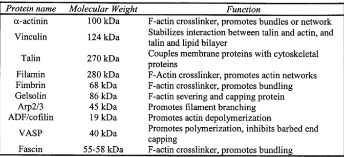
Inside the cell, the distribution between monomeric and filamentous forms of actin is regulated by the local concentration of both as well as the presence of capping, severing and sequestering proteins (Table 1.1). At the leading edge, conditions favor the formation of filaments in order to form protrusions (lamellipodia) that initiate cell migration. At focal adhesions, conditions keep a stable filament to provide a solid anchor and transmit forces along the cell. Previous work [12] has shown an increase in activation of several proteins at the focal adhesion site when the cell is mechanically stretched, but no quantitative data are available to describe how the binding kinetics are affected. As part of this work, an experimental method to quantify the binding kinetics between actin-binding proteins and actin filaments as tensile forces are applied to the filament is presented. The premise behind these studies is that application of force can change the energetics of some reactions, shifting the system to a different conformation. This conformation could result in a higher or lower binding affinity, which is what the goal of this project is aimed to study. The results of future experiments can elucidate which proteins are more active under force application. These could provide a better

(14)

understanding of the signaling cascade that transforms a mechanical stimulus into a bio-chemical reaction.

Protein name Molecular Weight Function

a-actinin 100 kDa F-actin crosslinker, promotes bundles or network

Vinculin 124 kDa Stabilizes interaction between talin and actin, and

talin and lipid bilayer

Talin 270 kDa Couples membrane proteins with cytoskeletal

proteins

Filamin 280 kDa F-Actin crosslinker, promotes actin networks

Fimbrin 68 kDa F-actin crosslinker, promotes bundling

Gelsolin 86 kDa F-actin severing and capping protein

Arp2/3 45 kDa Promotes filament branching

ADF/cofilin 19 kDa Promotes actin depolymerization

VASP 40 kDa Promotes polymerization, inhibits barbed end capping

Fascin 55-58 kDa F-actin crosslinker, promotes bundling

Table 1.1. Actin binding proteins, molecular weights (approximate) and functions 1.1.2 Optical Trapping

History

The concept of force generated by an incident beam of light on a surface has been studied since the seventeenth century. During that time, based on astronomical observations, the German astronomer Johannes Kepler hypothesized that the reason for the comet tails to point away from the sun was because the sun's radiation pushes them in that direction. Although this idea was considered extreme by that era, it set the stage for what was later known as the phenomenon of radiation pressure. In the late nineteen hundreds, James Maxwell, with his Theory of Electromagnetism, showed mathematically that light incident on a surface can actually generate a force, namely radiation pressure. The first experimental evidence of radiation pressure was obtained in 1901 by the Russian Pyotr Nikolaievich Lebedev [13] and by (unrelated experiments) the Americans Ernest Fox Nichols and Gordon Hull [14]. While their experiments were fairly simple (a light beam incident on a glass surface suspended in air by a fine torsional fiber), their results are the basis for the widely used technique of optical tweezers.

With the introduction of lasers during the 1960's, scientists found a way to generate a relatively small diameter beam with very high intensity. These high intensity laser beams can be focused to a tight, diffraction-limited spot that can generate forces to push, pull or

(15)

trap small objects with sizes ranging from a few to tens of micrometers depending on their optical properties. These observations prompted Arthur Ashkin [15-18] to perform pioneering experiments on optical tweezers. By 1986, Ashkin et al [19] demonstrated the first optical tweezers application by using a microscope objective to tightly focus a laser beam, attaining a stable three-dimensional trap. A year later Ashkin and others [20, 21] demonstrated several biological applications of optical tweezers by trapping bacteria, viruses and yeasts. These accomplishments initiated a technological revolution in manipulation of micron-sized particles that led to the sophisticated equipment used in optical tweezers.

Handles in optical tweezers

In biological applications, trapping the specimen is usually difficult because specimens usually have non-uniform geometry and/or optical properties. For this reason, the technique of using optical handles has been adopted. These handles are tethered to the specimen by means of protein-protein interactions. The most common types of handles are polystyrene and silica microspheres and they can be found commercially in a wide range of sizes and surface chemistry. These types of handles have much better optical properties than biological specimens, which enhance the trapping forces as well as trap stability.

Current applications

Optical tweezers have found widespread applications in the biological world. By using a near infrared laser, minimal damage to the biological specimen is obtained, as well as leaving the visible spectrum open for fluorescence microscopy. Current experiments range from probing mechanical properties of the cell, down to measuring single molecule events. In the future optical tweezers can be introduced in the nano-fabrication technology for its versatility and precise position control.

Applications in cell biology include studies in red blood deformation [22, 23], cell locomotion and lamellipodia formation [24, 25], focal adhesion formation [26], as well as manipulating single cells such as sperm, bacteria and viruses [20, 21, 27]. Optical traps are used in these applications since they provide a non-invasive method of probing cell characteristics.

(16)

At the molecular level, energy states are measured in terms of the thermal energy of a particle, which is expressed as kBT, where kB is the Boltzmann constant (1.38 x 1023 J/K) and T is the absolute temperature. At room temperature, thermal fluctuations have an energy of kBT 4 x 1021 J or 4 pN-nm. In these force and length scales optical traps have

a suitable application since they can usually apply forces in the range of 100 pN, and many protein conformational changes are just a few nanometers in range; therefore, the energy of the trap (- 500 pN-nm) dominates the thermal fluctuation energy. In this area, extensive work have been done on DNA stretching [28, 29] and unzipping [1]. Also, other studies include the mechanics of molecular motors such as kinesin [30-32] and myosin [33-35]. Results show that optical tweezers are an excellent tool for recording events at the single molecule level. For this reason, this tool was selected as the experimental equipment to study force dependent binding between actin filaments and actin binding proteins.

Optical trapping theory

As mentioned above, optical tweezers generate trapping forces by means of radiation pressure. _{When a laser beam passes through a dielectric particle several forces are} generated but the two most important are the scattering force and the gradient force [36]. The scattering force acts in the direction of propagation of the beam, and is proportional to the intensity of the incident beam. On the other hand, the gradient force is proportional to the spatial distribution of intensity of the beam and acts in the direction towards the higher intensity region. Since these two forces have components that act against each other, a force balance between them is required to obtain a stable optical trap.

The theoretical description of the forces acting on a particle can be catalogued in to three regimes: (1) object dimension much greater than the wavelength of light (d X) or Mie regime, (2) object dimension comparable to wavelength (d Z X), and (3) object dimension much smaller than the wavelength (d << X) or Rayleigh regime. In the Mie regime, particle trapping can be described using ray optics because the diffraction limited focus size is much smaller than the particle dimension. In the Rayleigh regime, particles can be represented as point dipoles and electromagnetic theory is required to describe the trapping phenomenon [36]. When the dimensions of the particle and the wavelength are

(17)

describe theoretically how the forces are generated. Unfortunately, this regime includes biological applications, where the characteristic size is - 1gm and the laser wavelength used is around 1064nm. At this wavelength cells and tissues exhibit very low absorption of light and minimal damage to the specimen is obtained. In this case, theoretical description of the optical trap is lagging behind experimental methods, and since favorable experimental results have been obtained, it seems that not much attention has been paid to the theory [37]. In the following paragraphs, a description of optical trapping in the Mie and Rayleigh regimes are presented.

Mie regime

In this regime, geometrical (or ray) optics provides a good approximation to describe the trapping force generation. When a ray of light passes through a

refractive medium, such as a dielectric microsphere, it in

is bent while entering and exiting the particle (Figure A

1.1). The momentum of the light is changed at each

bend, and by conservation of momentum of the system,

the momentum of the particle has to change by the Figure 1.1. Ray optics representation of gradient forces in optical trap. The same magnitude but opposite direction. Using green arrows represent the net force

generated by each ray. Inset:

Newton's Second Law, the rate of change of momentum change of the beam entering from the left of the particle.

momentum generates a force in the following way

F = - ~-.AO Equation 1.1

grad _t _At

From Figure 1.1, the horizontal components of the force cancel out and the net force acts toward the focus of the beam. Equation 1.1 only describes the gradient force, and it can be seen that it acts in the same direction as the momentum change of the particle. Further analysis is needed to obtain the scattering force, and only the result will be shown here. Notice that the particle will be pulled towards the focus of the beam only if the index of

refraction of the particle is greater than the index of refraction of the medium.

From Ashkin [18], in the Mie regime, the vector force F imparted by a single ray is described by

(18)

F n,,,L _T2[sin(20 -2e)+ R cos 20]

C 1 + R' 2 +2R cos 2c

nP f sin 20 T2

_[sin(29

_- _2e)₊_{R cos 20]} _{Equation 1.2}

C 1+R 2 + 2R cos 2c

where 0 is the angle of incidence, e is the angle of refraction, R and T are the Fresnel coefficients of reflection and transmittance respectively and i and

j

are the unit vectors in the direction parallel and perpendicular to the direction of the incident beam respectively. By definition the scattering force acts is the i component and the gradient force is the

I

component. Therefore, the j component gives a better description of the momentum change presented in Eq. 2.1. The net force acting on a particle is given by the vector sum of all the rays of the incident beam.

Rayleigh regime

Radiation pressure is generally expressed as

f - Equation 1.3

C

in terms of force per unit area where I is the intensity of the beam (power per unit area) and c is the speed of light, or in terms of force

P

F = -Equation 1.4

C

where P is the power of the incident beam. When considering the index of refraction of the solution medium, the force (and pressure) equation becomes

F = QM, Equation 1.5

C

where

Q

_{is a measure of the efficiency depending of type of beam (plane wave, spherical} wave, mode, polarization and the optical properties of the particle), and nm is the index of refraction of the medium.

In the Rayleigh regime, the electric field is considered uniform at the dielectric particle. Using this assumption, the scattering force is described as

F , = M ( , Equation 1.6

scatt

C where (9) _{is the time-average Poynting vector and}

(19)

= 8 I(ka)4 a 2 2 Equation 1.7

3 _{nr +2)}

is the scattering cross section of the Rayleigh sphere with radius a and index of refraction

nl, nr = n/n. is the relative index, and k = 2fnffm/A is the wave number of the beam.

Equation 2.6 shows that the scattering force acts in the direction of the propagating light. The gradient force is given by

grad V(E) Equation 1.8

where

2 2

a = n 2 r , Equation 1.9

is the polarizability of the particle and (E2) is the time-average of the dot product of the electric field [36].

The Mie and Rayleigh regimes provide a physical and mathematical model for how forces are generated to trap particles using laser beams. In practice, this theory is seldom used to determine the optical forces because

experimental setups are quite complex and not Energy Excited State all the optical properties of the specimens are

characterized. Instead, optical forces are

Emission determined experimentally using different

methods discussed section 3.1. Excitation -round State

1.1.3 Fluorescence Microscopy Reaction Coordinate

Many studies in biology require tracking Figure 1.2. Excitation and emission of fluorescent dyes. When the excitation beam hits an electron at very small particles (-nm) and/or events that ground state, it jumps to the higher energy excited state. In order to return to its ground state, energy are not capable of being observed with a light is released in form of light. Since there is some energy loss in the process, the emission microscope, even at high magnification. In wavelength is longer than the excitation wavelength; therefore, emission occurs at a general the smallest particle visible in a light different color.

microscope is on the order of the light source wavelength. For these cases, a particle can be labeled with a fluorescent dye that emits light when excited at a specific wavelength (Figure 1.2). By locating the center of the point spread function of the light emission, the position of the particle can be resolved even if the particle can not be visible because of it

(20)

size. This technique is called fluorescence microscopy. In this technique, a set of filters are used to block the excitation light from getting into the eye piece such that the image is generated only by the emission light from the dyes. The application of these fluorescent dyes is dictated by their properties of excitation and emission spectrum, and a wide selection of dyes is now available in the market to fit specific needs.

Although fluorescence microscopy has the advantage of being able to track particles at the nanometer and sub-nanometer range, this technique also has one disadvantage: a low signal-to-noise ratio (SNR). Since the whole specimen contains the fluorescent dyes, not only the region in the focal plane will get excited but also the rest of the solution in the laser path. This background fluorescence could decrease the ability of discerning between single events reducing the spatial resolution. A technique commonly used to reduce background effects is total internal reflection (TIR). With TIR, only a thin region of the specimen plane is excited by an evanescent wave, eliminating background fluorescence outside the focal plane. Total internal reflection fluorescence microscopy has made it possible for researchers to even record single molecule events [1, 36] that could not have been observed otherwise.

Principles of total internal reflection fluorescence microscopy (TIRFM)

When light travels from one medium to another, it can either get transmitted, reflected, absorbed or some combination of all of the above. To analyze this phenomenon, consider the case of an incident monochromatic plane wave with an electric field in the form of the complex exponential

E(F,t) =

N

₀i exp i(i 'r - t), Equation 1.10

where E0, is the amplitude vector (assumed constant in time), k, is the wave propagation vector, F is the position vector (in Cartesian coordinates), Ni is the temporal frequency of the wave, and t represents time. When this wave hits an interface at an incident angle 9, between two different media, the reflected and transmitted wave can be expressed as

Er(,t)= Eo exp i(kr F - ot + r, Equation 1.11

(21)

respectively, where q, and ., are the phase constants relative to ,, and for simplicity absorption is negligible. With further manipulation of these equations and by applying the laws of Electromagnetic Theory, two important laws are obtained:

0, = i, (Law of Reflection), and Equation 1.13

n, sin , = n, sin 0, (Snell's Law of refraction), Equation 1.14 where n is the index of refraction of each medium.

Since most of the time it is easier to measure power (or intensity) rather than the electric field of a wave, two dimensionless parameters are introduced to describe energy conservation across an interface. The first parameter is the reflectance R which is the ratio of the reflected power to the incident power:

P I AcosO I

R = -'- = ', ' =os Equation 1. 15

P _{IA cos9,} _I,

where A is the surface area of interface. The second parameter is the transmittance T which is similarly defined as:

_ P _ IAcosO, _.I, cos9,_S- _- _I.cs.- _Ics. _Equation_1.16

1 I , s Icos q

Since we are assuming that there is no energy loss at either medium, the following relation is obtained from energy conservation:

R+T = =1 -. Equation 1.17

Pi

From Snell's Law, if n, > n,, there is a critical angle of incidence 0, that will yield ,=

900, T = 0, and R = 1. With this condition, the theory presented here implies that all the

light is being reflected back into the first medium and none is being transmitted. This is the condition required to obtain total internal reflection. If the properties of the two media are known, then the critical angle is given by

0 = sin- 1- Equation 1.18

n,

Notice that the total internal condition can only be obtained if the light is propagating from an optically dense medium to a less dense medium. When the incident angle meets or exceeds the critical angle total internal reflection will occur and an evanescent wave is generated that propagates through the less dense medium.

(22)

Evanescent wave

Let the transmitted electric field be described by Equation 1.12, where

k ,i=kx+ky=(ksin 1)x +(kcos91)y Equation 1.19

and since it is assumed a polarized wave, there is no z-component (z is in the direction perpendicular to the incident plane). Using Snell's Law and applying the TIR condition

the following relations are obtained

k, = ik, n 2 2 i18 Equation 1.20

n,

k = ' sin9 . Equation 1.21

nt

Combining these equations with Equation 1.12, the transmitted electric field is described

by

E, =

Eot

exp(-

py)exp

i k xni sin 9, -cot Equation 1.22

nt

Where, for convenience, the phase factor was dropped. This expression shows that the evanescent wave decays exponentially in the direction normal to the interface, towards

the second medium with a decay constant length of 91. If glass (ni-1.5) and water (n=1.33) are used as media, a scaling analysis for each of the terms for the decay constant gives

n 2 sin2 12 n, ~ 1, n, ~ 1, sin G, ~ 1.-. 2 ~1 ~

n, _n

therefore, the evanescent wave becomes -95% extinct at a distance ~-/2. It is customary to excite at short wavelengths (488nm-514nm), resulting in an excitation thickness of

about -250nm. This thickness is small compared to the specimen height (-100pm), therefore only about 0.25% of the specimen height in solution is excited, eliminating most of the fluorescent background (Figure 1.3).

(23)

Excited Evanescent

Chromophores Wavefront

Excitation ea Glass coverslip

Figure 1.3. Schematic representation of TIRF.

An intriguing part of the evanescent wave is its energy source. If all the rays are being reflected back to the original medium, what is the energy source for the evanescent wave? For all the derivations presented here, an ideal infinite plane wave was considered, but in reality the optics and the laser source have finite size. This restriction gives rise to light diffraction which is not accounted for. Because of this phenomenon, some of the light will actually get transmitted to the second medium even at the TIR condition. This light "leakage" is the energy source of the evanescent wave.

(24)

(25)

Chapter 2: Experimental Equipment

For the proposed experiments, the equipment to be used consists of an optical trap combined with single molecule fluorescence microscopy capabilities. This equipment was designed and built around a commercially available microscope. The focus of this chapter is to present the design and construction of the experimental equipment.

2.1 Equipment Design, Construction and Capabilities

2.1.1 Design Objective

The objective of this work is to study how the binding kinetics between actin and actin binding proteins are affected by applying mechanical force to stretch an actin filament. The hypothesis behind these studies consists of a shift in the interaction energetics between two binding partners as application of force facilitates protein conformational changes. In order to perform these types of experiments, an instrument capable of both applying forces in the pico-Newton range and monitoring single molecule events is required. The design of this equipment is described below.

The objective of the design includes: (1) optical tweezers that can apply forces in the range of sub-pN to 100 pN; (2) position manipulation and detection in the nanometer range; and (3) single molecule fluorescence microscopy, with total internal reflection capabilities. All of these capabilities are integrated and automated by computer hardware and software (LabVIEW 6i; National Instruments Corp; Sunnyvale, CA), reducing human error during experiments. Automation of the system also provides high throughput of experimental runs, while recording real-time data at a fast rate ( > 1 kHz). The key feature of the instrument is simultaneous combination of optical trapping and single molecule fluorescence microscopy.

2.1.2 Overview of Equipment

The instrument consists of a microscope, three different laser sources and two isolated boxes with multiple optical elements: one box houses the optical trap and position detection subsystem as well as the laser sources; and a second box encloses the single molecule fluorescence detection subsystem. The first box is on an elevated optical bread board that has been enclosed for eye protection, dust elimination and air currents

(26)

reduction. The box also has clear lids for regular inspection of the optics. The fluorescence detection dark box is completely sealed in order to prevent outside illumination from leaking in. All the equipment is mounted on an optical floating table that serves as a damper for structural vibrations. In the following sections, the construction and the components used in the design of the instrument will be discussed.

2.1.3 General Overview of Optical Path

A schematic with the optical design is shown in Figure 2.1. There are four light

sources for the system: a bright field source as part of the microscope original design, and three laser sources, one for each of the functionalities of the instrument: position detection, trapping and fluorescent excitation. The optical path for each of the sources is described below.

single molecule fluorescence

ZSAPD JL / PH _F SAPD D4 FM2 S1 Pol2 D3

Jj

PSD Wol2 L4 z F1 iezo stage XWol 1 Pol1 DD video S3 camera _INIAM1 B' L 1 2 Yj 4 3 S5 WP T4 excitationtr FM1 _laser _{_} lamp diectio laser

Figure 2.1. Schematic of instrument design. Adapted from Lang et al

Microscope and bright field illumination

The instrument is based on the TE2000-U inverted microscope (Nikon Instruments, Inc., Melville, NY) with a 100X 1.40NA Plan APO, oil immersion objective (Nikon Instruments, Inc.) (Obj; Figure 2.1). The high numerical aperture of the objective allows for both optical trapping and objective side total internal reflection microscopy. The

optical tweezers )1 & position T1 S2-, I T2 AOD

(27)

fluorescence excitation laser at the specimen plane. To control the location of the specimen a manual, 2-axis stage (75-MS; Rolyn Optics, Covina, CA) and a xyz piezo stage (P-517.3CD; Polytec PI, Tustin, CA) were mounted on the microscope after modifying the microscope original design (see section 2.1.4 below). The microscope frame was secured to the optical table by means of two adapter plates affixed to the base.

A 100W Hg arc lamp (Nikon Instruments, Inc.) is used as the bright field source. The

amount of light that reaches the eyepiece is controlled by a set of polarizers (Poll, Pol2; Figure 2.1). These in conjunction with a pair of Wollaston crystals (Woll, Wol2; Figure 2.1) provide the phase contrast of the objects in the specimen plane. The light goes through the condenser (Con; Figure 2.1), the specimen slide and objective. Oil immersion objective and condenser are used. The image of the specimen plane is shuttled either to the eyepiece or a CCD video camera (CCD100; DAGE-MTI, Inc., Michigan City, IN) by means of a dial deflector inside the microscope. The CCD camera is connected to a monochromatic monitor (PVM-97; Sony Corporation of America, Parkridge, NJ), which sends the analog signal to a digitizer (Dazzle Digital Video Creator 150; Pinnacle Systems, Inc., Mountain View, CA) for capturing the image. The video-capture system described above works for both the bright field image and the fluorescence excitation image.

Position detection path

The source used for position detection is a near infrared fiber Bragg laser (980nm Optilock Pump; Coming Lasertron, Coming, NY; with LDC-3724B controller; ILX Ligthwave, Bozeman, MT) with up to 250 mW of power. For noise reduction, the laser power supply is located outside of the experimental room. The laser pump is coupled to an optical fiber and the output of the fiber is collimated using a beam collimator (F220FC-B; Thorlabs, Newton, NJ). The collimated beam is reflected through a pair of steering mirrors for alignment purposes (not shown in Figure 2.1). A 1:1 telescope (Ti; Figure 2.1) is used to provide manual control over relative displacement between the detection laser and the trapping laser. The beam then goes through a dichroic (Dl; Figure

2.1) that combines the detection beam with the trapping beam. After the dichroic, the

beam passes through a second 1:1 telescope (T3; Figure 2.1) that provides coarse position manipulation and focusing of both the trapping laser and the detection laser

(28)

simultaneously. As the beam enters the microscope region, it is reflected along the optical axis by means of another dichroic (D2; Figure 2.1) coated for near infrared wavelengths. Once in the optical axis, the objective (Obj; Figure 2.1) focuses the beam on the specimen plane. The beam is re-collimated by the condenser (Con; Figure 2.1) and reflected by a second dichroic (D3; Figure 2.1) along the detection branch. This path includes filter (Fl; Figure 2.1) that isolates the detection beam, and a lens (L4; Figure 2.1) that focuses the beam on the active area of a position sensing device (PSD; Figure 2.1). The PSD then transduces the intensity of the beam into x-y coordinates (see Position Detection section) represented by voltages, and this signal is monitored by a

computer.

Trapping laser path

A near infrared laser (Compass 1064-4000M; Coherent, Inc., Santa Clara, CA) with a

power output up to 4W is used to provide the trapping force. The laser source is located outside the experimental room (for noise reduction) and it is brought to the instrument by means of a single-mode, polarization maintaining optical fiber

(PMJ-3S3S-980-6/125-3-30-1; OZ Optics, Carp, Ontario). An output coupler collimates the beam exciting the

fiber. After being reflected by a pair of steering mirrors (not shown), the beam goes through a pair of acousto-optical deflectors (AOD; Figure 2.1) that provide fast and reproducible manipulation of the laser location on the specimen plane (see Position Manipulation Capabilities section). An iris is located right after the AOD's in order to block all the orders of the diffracted beam except the +1 order. The beam is then expanded by a 1:3 telescope (T2; Figure 2.1) in order to fill the back pupil of the objective to provide a larger intensity gradient, tighter focus and thus a larger trapping force. A dichroic mirror (D1; Figure 2.1) combines the trapping laser with the detection laser, and both go through the same path to the condenser. The objective focuses this beam in the specimen plane generating the trapping force. After the condenser, a set of filters (Fl; Figure 2.1) block the trapping laser from getting into the PSD.

Fluorescence excitation laser path

(29)

trapping laser, the laser source is located outside the experimental room and an optical fiber (QPMJ-33-488-3.5/125-3-30-1; OZ Optics) brings the beam into the room. The beam is sent to the microscope by a pair of steering mirrors. Then, the laser goes through a lens (L1; Figure 2.1, 15 cm focal length) that focuses the beam in the back focal plane of the objective. A movable mirror (Ml; Figure 2.1) reflects the beam into the filter cube

(FC; Figure 2.1) which sends the beam into the objective. The movable mirror facilitates

the option of setting epifluorescence or total internal reflection (see Total Internal Reflection Fluorescence Microscopy section). When the system is set for TIRF the return beam is blocked by a hard obstruction (B; Figure 2.1) to prevent it from returning to the

optical path.

As the excitation laser hits the specimen, fluorophores in solution get excited and emit light. This resulting emission is isolated by the filter cube which only passes the emission wavelengths. The fluorescence image is brought out of the microscope by a telescoping lens (T4; Figure 2.1) that enlarges the images 2.5 times. The beam enters a dark box with the single molecule fluorescence detection system (see Single Molecule Fluorescence Microscopy Capabilities section), and the image is collected by either the

CCD camera or the photodetectors.

2.1.4 Microscope Modifications

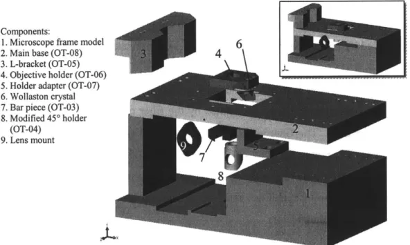
Since several modifications had to be made to the microscope to implement the optical trapping capabilities, a computer rendered virtual model of the microscope frame

(1; Figure 2.2) was created to facilitate component design. The objective turret, the filter

cube spin wheel and the original specimen stage were removed in order to free more working space. The design also took the advantage of the infinity-capability of the objective by extending the optical path. A one-inch-thick aluminum base (2; Figure 2.2) was designed to hold all the components that align the laser beams with the optical axis. The base was designed such that it provides stability to the microscope and its attachment uses existing threaded holes on the microscope frame. In order to mount this base to the microscope frame, the illumination pillar was removed and the base was secured to the back of the microscope. A bracket (3; Figure 2.2 ) was designed to hold the base at the front of the microscope frame. Then, the illumination pillar was mounted on top of the base, raising the optical system by one inch from its original height. The rest of the

(30)

components were designed to compensate for this additional height. A pair of adapters (4, 5; Figure 2.2) was made to hold both the objective and Wollaston prism, (6; Figure 2.2). These adapters were mounted onto the focusing platform of the microscope and replaced the objective turret. The design of these parts considered all the range of motion that the objective turret originally had plus additional clearance to avoid interference with other structural components.

Components:

1. Microscope frame model ₆

2. Main base (OT-08) 4

3. L-bracket (OT-05) 4. Objective holder (OT-06) 5. Holder adapter (OT-07) 6. Wollaston crystal 7. Bar piece (OT-03) 8. Modified 45* holder

(OT-04)

9. Lens mount

Figure 2.2. Microscope modifications (exploded view). Inset: Assembly view.

A dichroic mirror mounted on a modified 450 mirror mount (8; Figure 2.2) was used to reflect the incoming beam by 90' into the optical path. The 45*-mount was fixed to a bar piece (7; Figure 2.2) attached to the main base. This bar piece slides relative to the main base to align the incoming beam with the optical path. An additional threaded hole was made on the right side of the main base to hold one lens mount (9; Figure 2.2) from a telescope pair. Finally, a manual stage was mounted on top of the main base for coarse positioning of the specimen, and a nanometer-resolution piezo stage was placed on top of the manual stage for precise positioning (not shown in Figure 2.2).

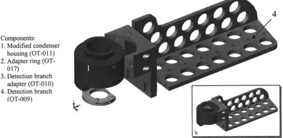
In addition, changes to the condenser were necessary for implementing the position detection system (Figure 2.3). A hole to the right side of the condenser housing (1; Figure 2.3) was made in order to image the specimen plane outside the main optical path.

(31)

reflecting the image horizontally towards the detection branch (4; Figure 2.3). This branch holds all the optical components for the position detection capabilities of the instrument.

4

Components:

1. Modified condenser

housing (OT-01 1) 2. Adapter ring

(OT-017)

3. Detection branch

adapter (OT-0 10) 4. Detection branch

(OT-009)

Figure 2.3. Condenser housing modification and detection branch (exploded view). Inset: assembly view

2.1.5 Position Detection Capabilities

The position detection system is based on the intensity profile generated by the scattering of a laser beam by a microsphere, and captured by a photodiode element. The element used in this instrument is a duo-lateral position sensing photodiode

(DL100-7PCBA; Pacific Silicon Sensor, Inc., Westlake Village, CA) with an active area of 1 cm x

1 cm, and for simplicity it will be referred as position sensing device (PSD). This type of photodiode transforms an intensity profile input to an output with the location of the centroid of the intensity profile in terms of voltages in two axes (V, and V) as well as the sum of voltages along both directions. The latter is used to normalize the former. The output signals are amplified and go through several filters to reduce external. An anti-alias filter (3384 Filter; Krohn-Hite Corp., Brockton, MA) set to one-half of the data collection further cleans the signal before being acquired by a 16-bit A/D board (PCI

6052E; National Instruments Corp; Austin TX). A calibration routine is then run to

convert the output voltages into actual positions in the specimen plane (see section 3.1.1). The PSD (Figure 2.1) is located at a conjugate optical plane of the condenser back focal plane in order to have the intensity profile independent of the focus location [38,

(32)

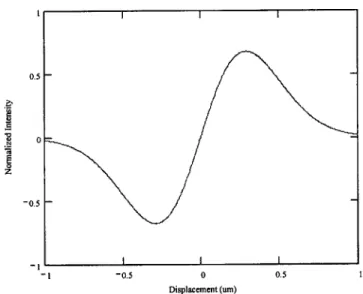
Newport, Irvine, CA). As the bead is displaced from the center of the detection beam waist, different scattering patterns are generated, and the photodiode converts these specific patterns into plane position of the bead. The mathematical derivation of the scattering profile of a laser beam through a microsphere is quite complicated, involving electromagnetic theory and optics design, and it is beyond the scope of this text. However, a model taken from literature will be compared to actual results to validate the instrument performance. Gittes and Schmidt [39] proposed a model to describe the intensity profile in one dimension as follows:

I+ -I1- 16 ica

1*- ~ 1 Equation 2.1

I+I- VE w where

G(u) = exp(- 2u2 _)exp(Y2

py, Equation 2.2

0

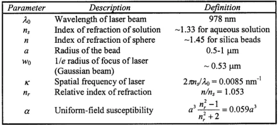
where x is the displacement of the center of the bead from the center of the trap. All the other parameters used are defined in Table 2.1.

Parameter Description Definition

& Wavelength of laser beam 978 nm

ns Index of refraction of solution -1.33 for aqueous solution

n Index of refraction of sphere -1.45 for silica beads

a Radius of the bead 0.5-1 pm

wo _{Ile radius of focus of laser} _{- 0.53 pm}

(Gaussian beam)

K Spatial frequency of laser 2 7msl/o = 0.0085 nm-1

nr Relative index of refraction n/ns = 1.053

n2_

a Uniform-field susceptibility a '2 = 0.059a3

n,2 + 2 Table 2. 1. Parameters used for position detection curve shape.

(33)

0.5 0 z -0.5 - ,I I -I--1 -0.5 0 0.5 1 Displacement (um)

Figure 2.4. Model of expected intensity plot versus bead displacement from the center of the trap.

Figure 2.4 shows the normalized intensity (arbitrary units) as a function of the bead displacement from the center of the trap for a bead radius of 0.5ptm and an estimated

focus waste of 0.53pm. From the graph it can be noticed that for a given intensity there are two different values of displacement which introduce ambiguity to position detection. To avoid this ambiguity instead of using the entire displacement region, only 80% of the distance between the low and high peaks is used. Between these peaks, there is a unique displacement for a given intensity value, and the absolute position of the bead can be determined. The actual results of the position calibration for the designed system are shown in section 4.1.

2.1.6 Position Manipulation Capabilities

For fast manipulation of the trapping laser at the specimen plane, a pair of orthogonal acousto-optic deflectors (DTD-276HB6; IntraAction Corp., Bellwood, IL) is employed. The AOD's are driven by a frequency generator (DVE-4010C9; IntraAction) controlled

by computer. The RF amplifier for these devices is placed outside the experimental room

for noise reduction. One of the AOD's controls the x-displacement while the other controls the y-displacement. The two are placed close together at a plane that is conjugate to the back pupil of the objective, such that deflection of the beam at this plane produces translation of the beam at the specimen plane.

(34)

Inside the AOD's, a pressure wave at a certain frequency is transmitted to a crystal producing a density pattern. This pattern acts as a sinusoidal optical grating, diffracting the beam into its different orders. The angle at which each order occur relative to the zero order is given by

= , Equation 2.3

where m is the diffracted order (m = ... ,-2,-1,0,1,2,...), Ao is the light wavelength,f is the

acoustic wave frequency and v is the velocity of the sound wave across the crystal. Note

that the zeroth order (m = 0) beam never changes its direction (Om = 0); therefore, it can

not be used for position manipulation. Instead, the first order beam is used because it carries more power than the higher order diffractions, and the other orders are block by placing an iris right after the AOD's. Equation 2.3 shows that by controlling the acoustic frequency

f,

the angle of the first order beam can be changed, providing control of the laser trap focus at the specimen plane. By using two orthogonal oriented AOD's, control in two dimensions is obtained.

One drawback from the AOD's is that by using the first order diffraction, some of the incoming power is lost, and by using two AOD's in series the power gets further reduced. To compensate for this loss, the intensity of the incoming beam has to be increased, but this is also limited by the optics that are located before the AOD's, for example the optical fiber, such that they do not get damaged by excessive levels of power. Also the power efficiency can vary depending on the frequency; therefore, to obtain a stable trap, only a limited range of input frequencies should be used. In this case the frequencies used for both x and y deflections are typically between 25.5-26.5 MHz.

On the other hand, AOD's have a very fast response time, limited only by the ratio of the acoustic velocity and the diameter of the laser beam [38]. For the instrument set up, the fastest response is dictated by the computer speed, the software being used, and the

communications ports.

2.1.7 Total Internal Reflection Fluorescence Microscopy Capabilities

In practice, there are two main configurations for implementing TIRF to a light microscope: prism method and objective lens method. The prism method uses a prism on I IIIIe

(35)

n

critical angle. With this configuration, the evanescent wave is generated at the top of the slide and it travels down the specimen. Some disadvantages of this method are restricted access to manipulate the specimen, and imaging the evanescent wave through the bulk of the specimen. For these reasons and geometrical restrictions, the objective lens method was implemented in the instrument. With this technique the excitation beam is brought to a tight focus at the back focal plane of the objective in order to have a collimated output beam from the objective and satisfy the critical angle condition. The angle of incidence is controlled by adjusting the distance between the back focal point and the optical axis; that is, higher angles are achieved by greater offset distances. This behavior can be demonstrated by using geometrical optics, the paraxial approximation (small

angles, i.e. sinO ~ 0) and the thin lens assumption. Consider the simple lens system in Figure 2.5, where a point source located at the back focal plane is imaged through the

lens. The light propagation is described by the matrix

0[,~[ 1 0 oi] 0 0

x L 0 1 "- f 1J

Lens Light propagation matrix from source to lens

where Oin and 0_out_{are the input and output beam angles respectively, and}

xin and x,, are

the distance from the optical axis of the input and output beam respectively. Notice that if the point source is located at the back focal plane, the output angle is independent of the input angle and the former becomes

-out

= - n Equation 2.4

f

where the minus sign indicates that the output rays bend towards the optical axis. Therefore, by controlling the location of the input beam, the output angle (or the incident angle) is manipulated.

(36)

Lens with focal length=f Point source

tput beam

SOptical axis

Figure 2.5. Optical system to demonstrate the realtions between point source location and output angle.

The system implemented to control the input location is depicted on Figure 2.6. A collimated beam enters the system and through a lens (1; Figure 2.6, and Li; Figure 2.1) that focuses the beam at the back focal plane of the objective. In order to maximize the excitation region, the focal length of the lens has to be as short as possible so that the back pupil of the objective is filled. Because of space limitations, the minimum focal length attainable was 12cm. To precisely focus the beam at the back focal plane of the objective, the lens is mounted on a 3-axes stage (2; Figure 2.6) with a range of 10mm in all three directions. The beam is then bounced from a mirror (3; Figure 2.6, and M1; Figure 2.1) mounted on a 1-axis stage (4; Figure 2.6), into a filter cube (5; Figure 2.6, and

FC; Figure 2.1). The dichroic of the filter cube sends the excitation beam into the

objective. The filter cube also serves as a filter, blocking the excitation beam from getting to the eyepiece and the imaging system. The angle of incidence at the specimen plane can be changed by moving the mirror stage (4; Figure 2.6) which offsets the focal point of the incoming beam from the optical axis. By moving the stage to either extreme, the TIR condition is obtained.

(37)

TIRF System:

1. Lens (KPX097 f=12cm, Newport) and 15

lens holder (LMRl, Thorlabs)

2. 3-axes stage (M-MT-XYZ, Newport) 7 3. Reflective mirror (02 MPQ 007/023,

Melles Griot)

4. 1-axis stage (MT-X, Newport)

5. Filter cube (Z488RDC or Z514RDC, Chroma)

6. Bottom plate adapter (OT-24)

7. Filter cube holders (M-MRLl.5, Newport)

8. Kinematic mount adapter (OT-25) 9. Kinematic mount (KMS/M and MH1,

Thorlabs)

10. Magnetic mount (KBlX) 11. Magnetic mount adapter (OT-22) 12. Side adapter plate (OT-23) 13. Filter cube adapter plate (OT-26)

14. Input beam (from source) 4

15. Ouput beam (to objective)

Figure 2.6. Schematic representation of TIRF system implemented in the Nikon TE2000-U microscope. For many applications controlling the location of the input beam is not enough to obtain the TIR condition because the maximum angle of incidence achievable is strictly governed by the objective physical limitations. This limitation is the numerical aperture

(NA) which is given by

NA = n sin 9 Equation 2.5

where n is the index of refraction of the medium (usually oil, n=1.55) and 9 is the half angle of the physical objective aperture from its focal point. Combining this equation with Snell's Law and the TIR condition a very important relationship is obtained:

NA = n, sin 0, = n, . Equation 2.6 Equation 2.6 shows that in order to obtain total internal reflection, the numerical aperture must be equal or greater than the index of refraction of the specimen medium. For the instrument, an objective with numerical aperture of 1.40 was used, which is enough for most aqueous solutions applications which index of refraction range between 1.33 and

1.35.

Once the TIR condition is obtained, the return beam has to be blocked so it does not interfere with the image formed by the emission of the fluorescent dyes. To address this situation a small hard stop is placed on top of the filter cube (B; Figure 2.1).

The light source being used is an Argon ion laser with variable wavelength (488nm to 514 nm) and maximum power output of 10 mW. Since different applications require

(38)

different power inputs, an optical system to control the power input was placed right after the laser source. The system consists of a combination of a beam splitter and a X/2 waveplate; therefore, by rotating the waveplate relative to the beam splitter, the amount of polarized light entering the microscope objective is precisely controlled.

Other features of the TIR design are its easy alignment, and its versatility of functioning at different wavelengths. By using the 3-axis stage, the 1-axis stage and the kinematic mirror mount, any input beam can be readily aligned with the microscope optical axis. Also, the system was designed such that filter cubes could be easily exchanged depending on the excitation wavelength to be used. In addition, the filter cube adapter plate (10) has a slot aligned with the optical axis for placing additional filters if necessary.

2.1.8 Single Molecule Fluorescence Microscopy Capabilities

The system for single molecule fluorescence microscopy is depicted in lower left side of Figure 2.1. Once the image of the fluorescence emission enters the "dark box", it can either be sent to a CCD video camera or the single molecule detection system by changing the setting of an electronic flipper mirror (FM1; Figure 2.1). To avoid excessive intensity from reaching the silicon avalanche photodiodes (SAPD; Figure 2.1) or the intensified camera, a shutter (S5; Figure 2.1) and a set of filters (F3; Figure 2.1) are placed at the entrance of the single molecule detection system. A second flipper mirror (FM2; Figure 2.1) is used to send the image to either the intensified camera or the SAPD's. Because very low light intensity is required, the intensified camera provides a way of actual visualization of the image, that otherwise with the regular CCD camera it could not be seen. A lens (L2; Figure 2.1) relays the image to the active area of the intensified camera. For the actual single molecule detection, the flipper mirror FM2 is lowered so that the image is directed towards the SAPD's. Before reaching the SAPD's, the beam goes through a pinhole (PH; Figure 2.1) which is located at a conjugate image plane. The purpose of the pinhole is to limit the size of the beam getting to the SAPD in such way that they only collect light from a very limited region, preventing them from getting saturated. The pinhole has a diameter of 300 pm which gets transferred to a size