How to define a rejection class based on model learning?

HAL Id: hal-02963115

https://hal.archives-ouvertes.fr/hal-02963115

Submitted on 9 Oct 2020

HAL is a multi-disciplinary open access

archive for the deposit and dissemination of

sci-entific research documents, whether they are

pub-lished or not. The documents may come from

teaching and research institutions in France or

abroad, or from public or private research centers.

L’archive ouverte pluridisciplinaire HAL, est

destinée au dépôt et à la diffusion de documents

scientifiques de niveau recherche, publiés ou non,

émanant des établissements d’enseignement et de

recherche français ou étrangers, des laboratoires

publics ou privés.

How to define a rejection class based on model learning?

Sarah Laroui, Xavier Descombes, Aurélia Vernay, Florent Villiers, François

Villalba, Eric Debreuve

To cite this version:

Sarah Laroui, Xavier Descombes, Aurélia Vernay, Florent Villiers, François Villalba, et al.. How to

define a rejection class based on model learning?. ICPR2020 - International Conference on Pattern

Recognition, Jan 2021, Milan, Italy. �hal-02963115�

How to define a rejection class based on model

learning?

Sarah Laroui1,2

,

,

,

,

, and

1

Team Morpheme, Inria CRISAM/Laboratoire I3S/Laboratoire iBV, Sophia Antipolis, France

2

Universit´e Cˆote d’Azur, Nice, France

3

Bayer SAS, Disease Control Research Center, Lyon, France

Abstract

In supervised classification, the learning process typically trains a classifier to optimize the accu-racy of classifying data into the classes that appear in the learning set, and only them. While this framework fits many use cases, there are situations where the learning process is knowingly performed using a learning set that only represents the data that have been observed so far among a virtually unconstrained variety of possible samples. It is then crucial to define a classifier which has the ability to reject a sample, i.e., to classify it into a rejection class that has not been yet defined. Although obvious solutions can add this ability a posteriori to a classifier that has been learned classically, a better approach seems to directly account for this requirement in the classifier design.

In this paper, we propose an innovative learning strategy for supervised classification that is able, by design, to reject a sample as not belonging to any of the known classes. For that, we rely on modeling each class as the combination of a probability density function (PDF) and a threshold that is computed with respect to the other classes. Several alternatives are proposed and compared in this framework. A comparison with straightforward approaches is also provided.

1

Introduction

In supervised classification, the learning process typically trains a classifier to optimize the accuracy of classifying data into the classes that appear in the learning set, and only them [1]. This framework fits many use cases. For example, in a medical context, the expert knows in advance that the data will be distributed among the healthy class and a given number of pathological classes. There are situations though where the learning process is knowingly performed using a learning set that only represents the data that have been observed so far among a virtually unconstrained variety of possible samples. For example, in a biological study where cells are cultivated in vitro in the presence of a chemical compound, the activity of such molecule can result in specific and remarkable morphological cellular changes collectively called a phenotypic signature. One might want to build a classifier ensuring the automatic recognition of known phenotypes, ensuring in the future a robust and valid clustering of such cases. In parallel, all new chemical treatment could lead to new morphological changes or phenotypes, which should be automatically assigned to the so-called rejection class. Another example is given by a genetic screen study where the different possible patterns induced by inhibiting a given gene are unknown. Obvious solutions can add this ability to a classifier that has been learned classically. For a k-Nearest neighbor classifier, a threshold on the distance to the neighbors can be used to reject samples that are too far [2, 3, 4]. For a Deep Neural Network, a function of the output layer can be defined so as to represent a confidence of the prediction. Applying a threshold on such a confidence allows to reject samples [5, 6]. Nevertheless, a classifier is a feature space splitter which focuses on optimizing the frontiers between classes without much attention to the space in-between classes or away from them. Therefore, a better approach seems to directly account for the requirement to possibly reject samples in the classifier design. In [7], a rejection option is defined on the output of a Convolutional Neural Networks (CNN). The rejection procedure is optimized based on three costs: the (negative) cost of making a good prediction, the cost of making a wrong prediction, and the cost of rejecting a sample, which is lower than when predicting wrongly. The procedure is optimal when it rejects as much bad predictions as possible while keeping as much good predictions as possible. It relies on thresholds which are estimated using a learning set.

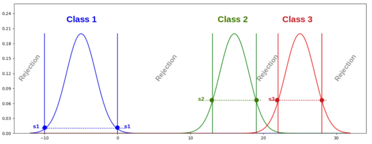
Figure 1: Illustration of the dependency of the FMF thresholds on the proximity between the classes using three Gaussians with the same variance.

This paper presents a method for supervised classification with a rejection class which accounts for the neighboring relationships between the known classes instead of classically defining a rejection procedure as a collection of independent, per-class decisions. The main steps are the model estimations for each class and the learning of thresholds based on inter-class relationships. The paper is organized as follows: Section 2 description of the proposed method, the decision rules and the proposals for establishing a model and a threshold specific for each class. In Section 3, a case study in the biochemistry domain and how our method is employed to classify in known class and reject samples which not belonging to any of the known classes. Then we will conclude based on the results obtained with the different methods.

2

Proposed method

The proposed learning strategy relies on class models where a model is a combination of a fuzzy member-ship function (FMF) (typically a probability density function (PDF)) on the data space and a threshold. For a sample s, if F is an FMF of a class, then F (s) is a real value between zero and one indicating how likely it is that s belongs to the considered class. The FMFs are learned independently for each class [8]. However, the thresholds are learned by taking into account the overlapping between the classes, thus inferring the possible location of new classes depending on the variability of neighboring classes (see Fig. 1). Finally, the prediction of a sample class is made by considering the responses from all the models. It can either fall into one of the classes used for learning or into the rejection class.

2.1

Notations and sketch of the proposed strategy

Let S be the learning set

S = ∪nc

i=1Si (1)

where Si is the subset of samples of class Ci and nc is the number of classes defined by the expert of

the domain. The samples of Si are denoted by si,j where j is the sample index between 1 and nSi. The sketch of the learning procedure is

• For all i, learn the FMF Mi of Ci based on Si;

• For all i and for a given k, learn a threshold Ti,k on Mi based on Mi, Si, and ∪j∈JkSj where Jk is defined in Eq. (2).

Jk⊂ Nc= {1, 2, . . . , nc}, i 6∈ Jk. (2)

Let us consider two options for Jk:

– If Jk is Nc\ {i}, then the threshold Ti on Mi is set to Ti,k;

– Otherwise the threshold Ti is set to some function of the Ti,k’s.

For some sample s, the sketch of the prediction procedure is • For all i, compute the hard membership response Mi(s) ≥ Ti;

• If all responses are false, then s is classified into the rejection class; • If only the jth _{response is true, then s is classified into class C}

j;

• If several responses are true, then classify s into the class j corresponding to the highest FMF value among the true responses (see Eq. (3)).

j = arg max

k|Mk(s)≥Tk

Mk(s) (3)

Section 2.2 details the proposed model learning approach. Note that Section 2.2.4 describes an alternative to the above prediction procedure.

2.2

Model learning

2.2.1 Fuzzy membership function (FMF)

A typical way to learn an FMF for the class Cibased on Siis to fit a Gaussian Mixture Model (GMM) [9]

to the samples of Si. The number of components of the mixture is a parameter whose optimization is

discussed in Section 3.6. For simplicity, it will be chosen identical for all the classes. Moreover, we decided to keep the Gaussian components isotropic. The position and variance of the components will be optimized classically using the expectation–maximization (EM) algorithm [9].

2.2.2 Thresholds on the FMFs

We propose to learn the threshold Tion the FMF Miof the class Ciby analyzing how this FMF responds

to “its own” sample set Si, naturally, but also to the sample sets of the other classes. There are then

two main options. (i) In the 1-vs-all approach, Ti is directly learned from Si and all the Sk’s, k 6= i. (ii)

In the 1-vs-some approach, a set of thresholds Ti,k’s is first learned from Si and some Sk’s, k ∈ Jk (see

Eq. (2)). Then the Ti,k’s are combined to produce the threshold Ti (see Section 2.2.3). One particular

case of the 1-vs-some approach is 1-vs-1 where nc − 1 thresholds are learned by considering all pairs

(Si, Sk), k 6= i.

For any of the 1-vs-? options, the problem is then to learn a threshold T? based on Mi, Si, and some

Sk’s, k ∈ Jk. For each sample s in the given sample sets, there is a value Mi(s). Ideally, this value is high

if s is in Si, and low otherwise. Besides, we can symbolically tag the samples of Si with the value one

and the samples of the other sets with the value zero. Then, we can plot the tag value against the value of Mi for each sample. Once presented this way, an idea that comes to mind to learn T? is to perform

a logistic regression [10]. The obtained regression sigmoid R moves from the zero-tag position up to the one-tag one. It seems appropriate to define the threshold T? on Mi as the inverse image of the fictitious

tag value 0.5

T? = R−1(0.5). (4)

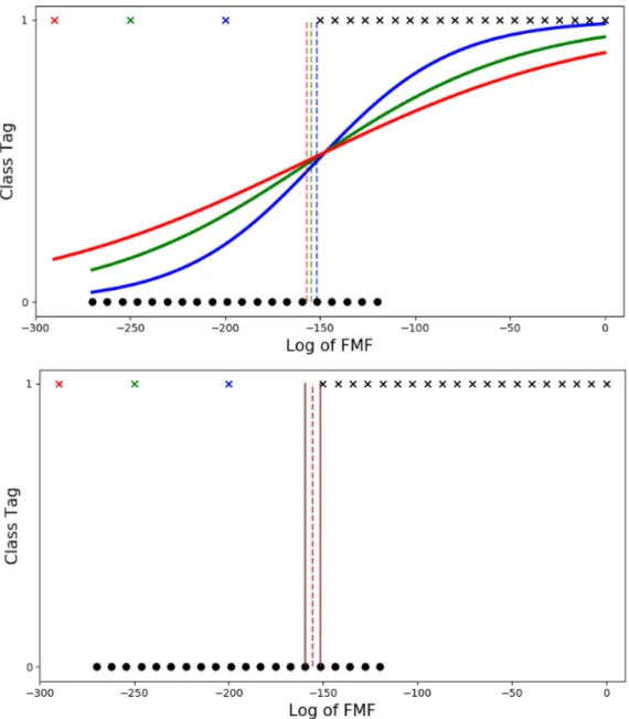
A potential drawback of this estimation is its sensitivity to outliers. Indeed, depending on the regular-ization applied to the regression problem, the transition of R from zero to one might be shifted in the presence of outliers (samples of Si with a very low value of Mi and samples of some Sk, k 6= i, with a

very high value of Mi). The severity of such a shift will depend on the horizontal position of the outliers

(see Fig. 2).

Thus, we propose an alternative method to learn T?using the number of misclassifications. If a sample

s belongs to Si, T? must be such that Mi(s) ≥ T? is true. If not, the prediction of s is a false negative.

Conversely, the condition Mi(s) < T? must be true if s belongs to the other samples sets. If not, the

prediction is a false positive. The threshold T?can then be expressed as the/a minimizer of

G(T ) =   #{s ∈ Si s.t. Mi(s) < T } − #{s ∈ Sk, k ∈ Jk s.t. Mi(s) ≥ T }    (5)

where #S is the cardinal of S. In practice, G does not have a unique minimizer so that T? cannot be

defined as arg minTG(T ). Instead, there is usually an interval [Tmin, Tmax] such that

∀T ∈ [Tmin, Tmax], G(T ) = min

Figure 2: FMF threshold learning illustrated on synthetic data with the two options: regression-based (top) and misclassification-based (bottom). Each color of curve and dashed thresholding line corresponds to a learning result with the learning set composed of the black cross and dot samples plus the cross sample of the same color. It can be observed that shifting the outlier position also shifts the threshold in the same direction when learning with regression, whereas the threshold learned using the misclassification criterion does not change (as long as the outlier does not enter the [Tmin, Tmax] as mentioned in the text).

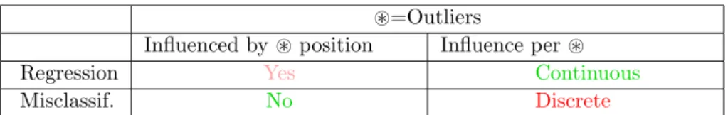
~=Outliers

Influenced by ~ position Influence per ~

Regression Yes Continuous

Misclassif. No Discrete

Table 1: Sensitivity to outliers of the regression-based and the misclassification-based estimations of T?

(see text for details).

Then, we propose to define T? as a function of Tmin and Tmax (see Fig. 2). The typical choice is the

average function

T?= (Tmin+ Tmax)/2. (7)

Regarding the sensitivity of the estimation (7) of T?to outliers, note that as long as no outlier moves into

the interval [Tmin, Tmax] (i.e., the values of Mifor the outliers remains outside this interval), the estimated

value is unchanged (see Fig. 2). However, the presence of an outlier influences the threshold learning in a discrete way, whereas its influence is continuous in the regression-based approach. By discrete, we mean that the presence of an outlier can make T?jump from one interval between samples (a [Tmin, Tmax]

interval) to a neighboring interval (see vertical dashed lines in Fig. 2). By continuous, we mean that the presence of an outlier will change T? in a smoother way.

The pros and cons of the regression-based estimation of T? and its misclassification-based estimation

are summarized in Table 1.

2.2.3 Combining the FMF thresholds in 1-vs-1 context

As explained in Section 2.2.2, in the 1-vs-1 context, nc− 1 thresholds Ti,k are learned by considering

all pairs (Si, Sk), k 6= i. The threshold Ti must then be computed as a function of the Ti,k’s. Three

straightforward options are the minimum, average, and maximum. Selecting the minimum among the Ti,k’s means that Tiis chosen according the class that is the farthest to Ci. This would increase prediction

errors for samples of the closer classes. Therefore, we propose to defined Tias the maximum of the Ti,k’s,

thus limiting the confusion between nearby classes. 2.2.4 Classification into known classes

The classification procedure into the rejection class has been defined in Section 2.1. The model-based procedure for classifying into known classes has also been described in the same section. We now suggest an alternative using an external classifier. Indeed, since classifiers such as CNN often exhibit very good classification performances in the no-rejection-class framework, they might be used advantageously in replacement of the model-based procedure whenever a sample has not been rejected (at least one hard membership response is true). Using a CNN would also provide us with the feature representation for our data.

3

Experimental results

3.1

Biological context

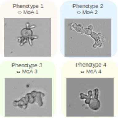
Botrytis cinerea is a reference model of filamentous phytopathogen fungi. We have observed that some anti-fungal molecules associated to an hypothesis of Mode of Action (MoA) can lead to characteristic morphological changes, or phenotypic signatures (see Fig. 3). In order to recognize and characterize the different phenotypes and associate them with the various modes of action, images are acquired by transmitted light microscopy after 24 hours of culture in the presence of molecules. Then, the images are labeled by an expert according to the observed phenotype.

3.2

Feature vectors for model estimation

3.2.1 Deep Neural Network (DNN)

Instead of hand-crafting features, we decided to take advantage of the feature learning capability of Convolutional Neural Networks (CNN). As mentioned in Section 2.2.4, we will also used the CNN for its predictions on non-rejected samples.

Figure 3: Four different classes observed on Botrytis cinerea model: four known characteristic phenotypes associated with different modes of action linked to different antifungal chemical families.

For the sake of simplicity, we chose to rely on the transfer learning [11] property of DNNs by using MobileNet [12] pre-trained on the ImageNet database [13]. The feature learning layers were frozen while the classification part was removed, replaced with one corresponding to our classification problem into four classes, and trained on our data. The raw data were 2160x2160-pixel grayscale images, collectively denoted by D. Each image was divided into 16 sub-images of 500x500 pixels, then rescaled to 224x224 pixels to fit the input shape of MobileNet. The rescaled sub-images of an image I are denoted by Ik, k ∈ [1..16].

3.2.2 Selected features

Once MobileNet re-trained on our data (see Section 3.2.1), each sub-image could be represented by the feature vector produced by MobileNet from its rescaled version. Let us see now the two proposed options for feature vector definitions.

Bottlenecks The term ”Bottleneck” classically refers to the output of the last layer before the classi-fication part of the network usually made of one or more dense layers. This is the straightforward option for feature vector definition. In MobileNet, this output is a 1001-dimensional vector, which we believe is too high to properly learn our class models. Therefore, a dimension reduction was performed.

Two approaches were evaluated: Principal Component Analysis (PCA) [14] and an approach based on variable importance (VI) as defined in supervised classification [15]. The latter one consists in computing the variable importance measure of each component of the feature vector definition. This is conveniently provided by publicly available Random Forest libraries [16], for example. The features were ranked from highest to lowest importance, and the k most important features were retained for further processing. Classically, the same procedure was applied to PCA-transformed features where variance plays the role of variable importance. In both case, the number k of retained features is a parameter that must be optimized.

Output layer Here, we suggest that the vector of the output layer of a DNN can be viewed as a feature vector instead of viewing it as an informative classification response from which to compute the prediction. Each component reflects a form of confidence that a sample belongs to the corresponding class. It has a value between zero and one, and the sum of all the components is normalized to one. Whenever one

Figure 4: Fitting a Gaussian onto the histograms of the four features for the samples of one given class: (top row) original data and (bottom row) symmetrized data. The Gaussians better approximate the original data (abscissa between 0 and 1) when fitted onto the symmetrized data.

component is very close to one (while the others are therefore close to zero), the classification response has only a single reasonable interpretation. However, when there is no clear maximum among the components, the way the component ”budget” of one is distributed among them might be interpretable by another classifier in order to correctly classify the corresponding sample. The use of the output layer as a feature vector follows from this hypothesis.

Let us study the vectors of the output layer for all the samples of a class. The histogram of the values of the component associated with the correct class will certainly have high values toward one and low ones toward zero. The opposite happens for the components associated with the other classes. In either case, the histogram looks like a truncated version of a hypothetical symmetric histogram centered on one or zero. As a consequence, if these vectors were to be used as-is as samples to learn a GMM, the mismatch between the non-symmetric component distribution and the symmetry of the Gaussian basis functions would certainly degrade the quality of the model fitting (see Fig. 4). In order to improve the fitting quality, we propose to symmetrize the component distribution by sample duplication. Let s be a sample

s = (s1, s2, . . . , sd)T. (8)

If the first component s1 is greater or equal to 0.5, then a new sample with a component s0i = 2 − si is

created. If si< 0.5, then the component of the new sample is equal to −si. This procedure is repeated for

both the sample and the newly created one with the second component. And again until the component sd. At each step, the number of samples is multiplied by two. In the end, the symmetrized sample

set contains 2d _{more samples then originally. In our case, the output vectors are 4-dimensional, so the}

symmetrized set has 16 more samples. Note that once the model fitting is done (see Fig. 4), the samples created for symmetrization are simply discarded and the learned model can be used normally on the original samples.

3.3

Learning set for model estimation

In practice, we noted that, because of the sparse and non-uniform spatial distribution of the fungi, some sub-images were empty while others were densely populated with objects. The feature vectors of these sub-images correspond to outliers in the learning set. Therefore, we moved from a learning set at the level of sub-images to an image-level learning set

L = {m(f (I1), f (I2), . . . , f (I16)) | I ∈ D} (9)

where f denotes the mapping between a rescaled sub-image and its feature vector as produced by Mo-bileNet, and m is the vector of per-component medians of its (vector) arguments (normalized between 0 and 1). The number of samples per known class in L was 233, 225, 297 and 441 for classes 1 to 4 respectively. Classically, a part of L will be used for training, a part will be used to assess the accuracy of the proposed method on the known classes in a cross-validation framework. Moreover, 638 samples that were identified by an expert as not pertaining to any of the four known classes will be used to assess the ability of the proposed method to classify into the rejection class.

3.4

Model estimation

As mentioned in Section 2.2.1, the learning of the FMFs of the class models was performed using a GMM fitting. A Gaussian is characterized by its mean and covariance matrix. Three constraint levels on the covariance matrix were tested: spherical (the covariance matrix is diagonal-constant), diagonal (the covariance matrix is diagonal), and full (no constraint on the covariance matrix). Each component of the mixture has its own covariance matrix. If k is the number of components selected for the fitting and d is the number of dimensions of the sample space, then the number of GMM parameters to estimate is k(d + 1) for spherical, k(d + d) for diagonal, and k(d + d(d + 1)/2) for full.

3.5

CNN-based rejection class

3.5.1 Method CNNro

The proposed method was compared to the method in [7], denoted here by CNNro. This work defines a rejection option that can be applied to any classical classifier. The rejection option is based on a function defined to estimate the classification reliability of a sample. Then a threshold is learned on this function so as to reject as much wrongly classified samples as possible while keeping as much correctly classified samples as possible. This is expressed as the optimization of a performance measure P with respect to a threshold σ. In practice, the authors propose to implement their approach for a CNN and use two sets of reliability function and threshold in cascade. The first reliability function, ΨA, corresponds to the

maximum of the output layer. The second function, ΨB, corresponds to the difference between the two

largest values of the output layer. A sample s is rejected if ΨA(s) < σA, or else if ΨB(s) < σB, where

σAand σBare optimized according to P on the whole sample set and on the samples that have not been

rejected by ΨA, respectively. This optimization depends on a parameter called the normalized cost CN

(see Section 3.6).

3.5.2 Methods CNNa and CNNr

We also compared the proposed method with two straightforward ways to reject a sample with a CNN. (i) If the highest value among the output neurons is lower than some threshold, then the sample is classified into the rejection class. Otherwise, it is classified into the class corresponding to the neuron as usual. Let us call this procedure the absolute-threshold rejection method and denote it by CNNa. Alternatively, (ii) the thresholding can be made on the difference between the two highest values among the output neurons. This procedure is called relative thresholding and denoted by CNNr. In both cases, a threshold TCN N ?

must be learned, ? being either “a” or “r”. In order to perform this learning in the same conditions as the ones for the proposed method, the samples of the unknown class were not used. Instead, each one of the four known classes was used in turn as if unknown (say class C4), the three others playing their

actual role of known class (C1, C2 and C3). This means that a new CNN classifier has to be learned

for just the current three known classes. It was done in a transfer learning mode: keeping the feature learning layers, cutting out the classification layers, adding new classification layers with three output neurons, and optimizing only this newly added part of the CNN. Afterwards, a threshold TCN N ?(1, 2, 3|4)

rejection classes (weight: relative number of samples per class as usual). In practice, a hundred thresholds between 0.3 and 1 were tested. In the end, four thresholds were learned: TCN N ?({1, 2, 3, 4} \ {i}|i) where

i ∈ [1..4]. The threshold TCN N ?was computed as a function of the TCN N ?(· · · |·). In our application, the

median led to the best results (where the median of four values is simply the average of the two middle ones).

3.6

Results and analysis

The experimental results were averaged over a repeated random sub-sampling cross-validation of 20 rounds. In each round, the data corresponding to known classes were randomly split into a training set (50%), a validation set used for parameter optimization (30%), and a test set for the estimation of classification accuracies (20%). In each training, validation and test set, we have respected the balance between the classes. Note that the data corresponding to unknown classes were used only for testing.

As a reminder, the images were represented by the bottleneck features or the output of a CNN. When dealing with bottleneck features, dimension reduction was performed using variable importance or PCA, and the optimal reduced dimension was selected using brute force search in the interval [10, 300] with a step of 10 from 10 to 100 and a step of 100 afterwards. When dealing with the CNN outputs, the data were symmetrized or not. The FMFs of the classes were estimated using GMMs. We tested different types of covariance parameters, we have kept the ones that give the best results. Note that the number of Gaussian components was optimized globally for all the classes. The optimal number was selected using brute force search in the interval [1, 11]. The thresholds on the FMFs were estimated using either logistic regression or a misclassification score, in a 1-vs-all or 1-vs-1 context. The classification accuracies obtained in all these experimental settings are presented in the table 2.

Methods Features Results

Threshold learning Regression Misclassif. 1-vs-all 1-vs-1 1-vs-all 1-vs-1 Proposed Bottleneck (Spheric GMM) Var. importance Known 93 91 87 88 Rejection 80 85 87 87 Dimension 90 90 100 50 Nb components 11 11 11 11 PCA Known 89 86 81 83 Rejection 65 72 77 75 Dimension 40 30 30 30 Nb components 11 11 11 11 Output (Diagonal GMM) Original Known 94 82 72 76 Rejection 28 88 90 87 Dimension 4 Nb components 10 10 10 9 Symmetrized Known 93 81 70 75 Rejection 92 100 99 99 Dimension 4 Nb components 9 10 9 11 CNNro N/A Known 65 Rejection 100 CNNa Known 65 Rejection 81 CNNr Known 70 Rejection 75 CNNmax Known 91

Table 2: Classification accuracies as percentages for the various experimental settings. The actual values were rounded to the closest integer. In particular, values of 100 in the table correspond to accuracies above 99.5%. The “Known” rows correspond to the accuracy on the known classes and the “Rejection” rows correspond to the other, unknown ones (the rejection class from the classifier point of view). A parameter of the GMM corresponds to the type of covariance used. Diagonal is the case where the contour axes are oriented along the coordinate axes and the eccentricities may vary between components. Spherical is a ”diagonal” situation with circular contours. CNNro corresponds to the method proposed in [7] (see Section 3.5.1). CNNa denotes the absolute-threshold rejection method for a CNN. CNNr denotes the method of rejection based on relative thresholding. CNNmax refers to MobileNet learned classically on the four known classes. Therefore, it has no sample rejection capability.

They were computed separately for the test samples of the known classes (see “Known” rows) and the samples of the other, unknown classes (which, as mentioned earlier, were never used in training or validation; See “Rejection” rows). As previously explained, the classification into known classes can be done by the proposed method or falling back to an additional classifier, here the CNN used to compute the feature vectors of the data (see Sections 2.2.4 and 3.2.1).

When using the bottleneck features with the proposed method, the best results are always obtained when reducing the feature space dimension based on variable importance. Within this context, the best results are always obtained with the regression-based threshold learning. Within this “sub-context”, the best results are obtained in the 1-vs-1 context. When using the output features, the best results are always obtained when symmetrizing the data (which allows a better GMM fitting). Within this context, the best results are always obtained with the regression-based threshold learning. Within this “sub-context”, the best results are obtained in the 1-vs-all context. Overall, the best setting corresponds to the 1-vs-all regression-based threshold learning on FMFs estimated on symmetrized output features. The accuracies were 93% and 92% on the known samples and the samples of the new classes, respectively.

The proposed method was compared with the method CNNro (see Section 3.5.1). To find the two thresholds σAand σB, we tested a range of values for the normalized cost CN, which is given by

CN =

Ce

Cr

− 1 (10)

where Ce is the cost of a single misclassification and Cr is the cost of a rejection. Using cross-validation

on 50 folds, we obtained the best classification accuracies on known and new class samples for CN equal

to 25. The optimal values for σAand σBwere 0.94 and 0.91, respectively. These accuracies were 65% on

the known samples and 100% on the samples of the new classes (values rounded to the closest integer). The proposed method is largely better on the known samples (+28%). It performs worse on the new samples, but not dramatically (92% versus 100%). Together with the fact that the proposed method is also more balanced (1% difference between known and new versus 35% for CNNro), it can be concluded that it is significantly better.

The proposed method was also compared with the CNN with absolute threshold method (CNNa) and the CNN with relative threshold method (CNNr) (see Section 3.5.2). In the learning stage, the following thresholds were found: {0.70, 0.72, 0.84, 0.98} for TCN N a(· · · |·), and {0.49, 0.52, 0.73, 0.96} for

TCN N r(· · · |·). In both cases, there is a significant variability among the thresholds. It probably reveals

that the four known classes do not overlap each other equally. A tentative explanation goes as follows: if the rejection class is far away from the three known classes, the CNN output for its samples will certainly have fairly low values for all of the output neurons. The rejection procedure can then afford a low threshold. On the contrary, if the rejection class overlaps significantly the three known classes, the CNN output for its samples will certainly be closer to the outputs for the samples of the known classes, that is, one output neuron with a value close to one, the others with a value close to zero. In this case, the rejection procedure is forced to use a high threshold. In practice, taking the median of these thresholds led to the best results. So we used TCN N a = 0.81 and TCN N r = 0.675. The proposed method with

its best settings compares very favorably to these two straightforward approaches to defining a rejection class with a CNN classifier. Indeed, it provides accuracies higher by 10 to 25% for both the rejection and the known classes. Besides, it is even on par with the (unmodified) learned CNN (denoted by CNNmax) on the known classes with an accuracy of 93% versus 91% for CNNmax (see Table 2).

4

Conclusion and perspectives

We proposed a method of rejection class based on model learning in a supervised context. It follows a general strategy with three main steps: model learning independently for each class, threshold learning based on class interactions, and prediction procedure. Although the focus is on sample rejection, the method can also be used for classification into the classes known at the time of learning.

In the studied application, the proposed method provided very good classification accuracies for both the rejection class and the known classes. On the known classes, it proved to be equally effective than a CNN classifier. The significantly lower performances of two straightforward approaches to defining a rejection class with a CNN classifier tend to show that defining a rejection class should probably not be considered as an afterthought, but rather be part of the classifier design.

Regardless of the performances, let us note the main practical differences between bottleneck and output features. With bottleneck, reducing the feature space dimension will often be necessary. However, the features do not have to be learned again if a new class is formed. With the output layer, the feature

space dimension is reasonable. Nevertheless, adapting and re-training the classification part of the CNN is mandatory whenever new classes enrich the expert knowledge.

As noted above, the performances in our application are very satisfying. However, the accuracy is slightly better for samples of known classes with the bottleneck features. Conversely, the accuracy is better for rejected samples with output features (except the notable “Original/Regression/1-vs-all” case). Future works will concentrate on understanding and reducing or removing these biases.

Experimentally, there is an improvement we would like to consider. Here, the model fitting to learn the FMFs was done in the same conditions for all the known classes. Namely, the GMMs were optimized for the same number of components for all the classes. Letting the number of components be also optimized on a per class basis could improve the results further. In particular, the number of components could be estimated using an RJMCMC algorithm [17], although it would imply a high computational time.

References

[1] D. Siegismund, V. Tolkachev, S. Heyse, B. Sick, O. Duerr, and S. Steigele, “Developing deep learning applications for life science and pharma industry,” Drug Res (Stuttg), vol. 68, no. 06, pp. 305–310, 2018, 305.

[2] B. Dubuisson and M. helene Masson, “A statistical decision rule with incomplete knowledge about the classes, ”pattern,” 1993.

[3] M. E. Hellman, “The nearest neighbor classification rule with a reject option,” IEEE Trans. Systems Science and Cybernetics, vol. 6, pp. 179–185, 1970.

[4] C. Dalitz, “Reject options and confidence measures for knn classifiers,” Schriftenreihe des Fachbere-ichs Elektrotechnik und Informatik der Hochschule Niederrhein, vol. 8, pp. 16–38, 01 2009.

[5] C. Chow, “On optimum recognition error and reject tradeoff,” IEEE Transactions on Information Theory, vol. 16, no. 1, pp. 41–46, January 1970.

[6] G. C. Vasconcelos, M. C. Fairhurst, and D. Bisset, “Investigating feedforward neural networks with respect to the rejection of spurious patterns,” Pattern Recognition Letters, vol. 16, pp. 207–212, 1995.

[7] C. D. Stefano, C. Sansone, and M. Vento, “To reject or not to reject: that is the question-an answer in case of neural classifiers,” IEEE Trans. Systems, Man, and Cybernetics, Part C, vol. 30, pp. 84–94, 2000.

[8] A. Brew, M. Grimaldi, and P. Cunningham, “An evaluation of one-class classification techniques for speaker verification,” Artificial Intelligence Review, vol. 27, no. 4, pp. 295–307, 2007.

[9] C. Biernacki, G. Celeux, and G. Govaert, “Assessing a Mixture Model for Clustering with the Integrated Classification Likelihood,” INRIA, Tech. Rep. RR-3521, Oct. 1998. [Online]. Available: https://hal.inria.fr/inria-00073163

[10] S. Sperandei, “Understanding logistic regression analysis,” Biochemia medica, vol. 24, no. 1, pp. 12–18, Feb 2014. [Online]. Available: https://pubmed.ncbi.nlm.nih.gov/24627710

[11] H.-C. Shin, H. R. Roth, M. Gao, L. Lu, Z. Xu, I. Nogues, J. Yao, D. Mollura, and R. M. Summers, “Deep convolutional neural networks for computer-aided detection: Cnn architectures, dataset char-acteristics and transfer learning,” IEEE transactions on medical imaging, vol. 35, no. 5, pp. 1285– 1298, 2016.

[12] A. G. Howard, M. Zhu, B. Chen, D. Kalenichenko, W. Wang, T. Weyand, M. Andreetto, and H. Adam, “Mobilenets: Efficient convolutional neural networks for mobile vision applications,” 2017. [13] J. Deng, W. Dong, R. Socher, L.-J. Li, K. Li, and L. Fei-Fei, “ImageNet: A Large-Scale Hierarchical

Image Database,” in CVPR09, 2009.

[14] I. Jolliffe, Principal Component Analysis, ser. Springer Series in Statistics. Springer New York, 2006. [Online]. Available: https://books.google.fr/books?id=6ZUMBwAAQBAJ

[15] A. Criminisi, E. Konukoglu, and J. Shotton, “Decision forests for classification, regression, density estimation, manifold learning and semi-supervised learning,” Tech. Rep. MSR-TR-2011-114, October 2011. [Online]. Available: https://www.microsoft.com/en-us/research/publication/decision-forests-for-classification-regression-density-estimation-manifold-learning-and-semi-supervised-learning/ [16] F. Pedregosa, G. Varoquaux, A. Gramfort, V. Michel, B. Thirion, O. Grisel, M. Blondel, P.

Pretten-hofer, R. Weiss, V. Dubourg, J. Vanderplas, A. Passos, D. Cournapeau, M. Brucher, M. Perrot, and E. Duchesnay, “Scikit-learn: Machine learning in Python,” Journal of Machine Learning Research, vol. 12, pp. 2825–2830, 2011.

[17] P. J. GREEN, “Reversible jump Markov chain Monte Carlo computation and Bayesian model determination,” Biometrika, vol. 82, no. 4, pp. 711–732, 12 1995. [Online]. Available: https://doi.org/10.1093/biomet/82.4.711