HAL Id: hal-01917792
https://hal.archives-ouvertes.fr/hal-01917792
Submitted on 9 Nov 2018
HAL is a multi-disciplinary open access
archive for the deposit and dissemination of
sci-entific research documents, whether they are
pub-lished or not. The documents may come from
teaching and research institutions in France or
abroad, or from public or private research centers.
L’archive ouverte pluridisciplinaire HAL, est
destinée au dépôt et à la diffusion de documents
scientifiques de niveau recherche, publiés ou non,
émanant des établissements d’enseignement et de
recherche français ou étrangers, des laboratoires
publics ou privés.
Quantifying the diversity in users activity: an example
study on online music platforms
Rémy Poulain, Fabien Tarissan
To cite this version:
Rémy Poulain, Fabien Tarissan. Quantifying the diversity in users activity: an example study on online
music platforms. SNAMS-2018 - The Fifth International Conference on Social Networks Analysis,
Management and Security, Oct 2018, Valence, Spain. pp.3-10. �hal-01917792�
Quantifying the diversity in users activity: an
example study on online music platforms.
R´emy Poulain
Sorbonne Universit´e, CNRS,Laboratoire d’Informatique de Paris 6, LIP6, F-75005 Paris, France
Remy.Poulain@lip6.fr
Fabien Tarissan
Universit´e Paris-Saclay, CNRS, ISP, ´
Ecole Normale Suprieure de Paris-Saclay Cachan, France
fabien.tarissan@ens-paris-saclay.fr
Abstract—Whether it be through a problematic related to information ranking (e.g. search engines) or content recommen-dation (on social networks for instance), algorithms are at the core of processes selecting which information is made visible. Those algorithmic choices have in turn a strong impact on users activity and therefore on their access to information. This raises the question of measuring the quality of the choices made by algorithms and their impact on the users. As a first step into that direction, this paper presents a framework to analyze the diversity of the information accessed by the users.
By depicting the activity of the users as a tripartite graph mapping users to products and products to categories, we analyze how categories catch users attention and in particular how this attention is distributed. We then propose the (calibrated) herfindahl diversity score as a metric quantifying the extent to which this distribution is diverse and representative of the existing categories.
In order to validate this approach, we study a dataset record-ing the activity of users on online music platforms. We show that our score enables to discriminate between very specific categories that capture dense and coherent sub-groups of listeners, and more generic categories that are distributed on a wider range of users. Besides, we highlight the effect of the volume of listening on users attention and reveal a saturation effect above a certain threshold.
Index Terms—Network analysis, Tripartite graph, Diversity, Online music platform
I. INTRODUCTION
Online networks and digital platforms have become more and more essential in our everyday life. Not only do they shape our interactions in the real world but they also constrain our actions in virtual spaces enabled by Internet and the Web. At a time when online data are systematically processed by online platforms, the traces left by users contain key information revealing their behaviour and taste, which led most of the firms relying on digital platforms to propose algorithmic recommendations to their users.
This activity is at the core of intense debates, such as the exploitation of private data [1], the impact of search engines on elections [2], the dissemination of fake news [3] or filter
This work is funded in part by the European Commission H2020 FET-PROACT 2016-2017 program under grant 732942 (ODYCCEUS), by the ANR (French National Agency of Research) under grants ANR-15-CE38-0001 (AlgoDiv), by the Ile-de-France Region and its program FUI21 under grant 16010629 (iTRAC).
bubble phenomena on social media [4]. As a consequence, this increasing use of digital platforms and their recommendation systems has led the scientific community to focus on the impact of algorithmic decisions on user’s behaviour [5], [6], [7], [8].
In this context, one particular question is related to the diversity of information proposed to users [9], [10], [11], [12]. Indeed, whether it be in the context of economic rec-ommendations (suggestion to purchase an item in Amazon) or news recommendations (suggestion to read a post in Newsfeed or an article in online media), algorithms strongly affect what is made visible to the users. One wonders in turn whether the choices made by the platforms to make certain information visible is representative of the diversity of existing information.
In this paper, we propose an approach exploiting the net-work structure generated by users activity in order to reveal the diversity of the information accessed by the users. We propose a new metric called (calibrated) herfindahl diversity in order to quantify this diversity and we show its relevance in the context of online music platforms, enabling in particular to discriminate between different behaviours.
The rest of the paper is organized as follow. After describing the formalism used to represent the activity of a user, we present our score measuring its diversity (Section II) and the information contained in the dataset on which we conduct the analysis (Section III). Then, we show how our metric can be used to analyze both the diversity of the music audience (Section IV) and the one of users attention (Section V). We finally conclude the paper and open the discussion on possible extensions and generalizations of the approach (Section VI).
II. BACKGROUND
In this section we provide all necessary background for the formal analysis of users activity. We start by defining tripartite graphs (Section II-A) and then propose the herfindahl diversity index (Section II-B).
A. Tripartite graph
A bipartite graph is a graph with two disjoint sets of nodes and such that links relate a node in one set to a node in the other set. Formally, it is defined by a triplet B = (>, ⊥, E)
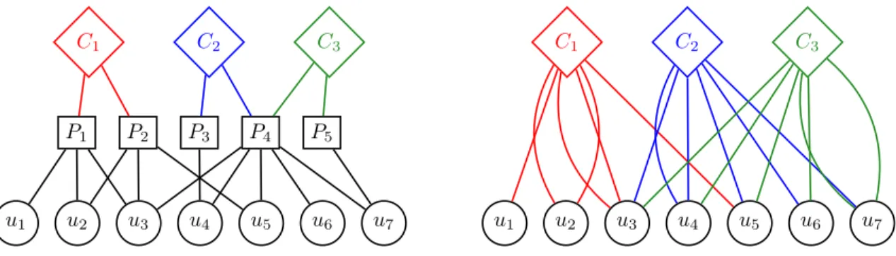
C1 C2 C3 P1 P2 P3 P4 P5 u3 u2 u1 u4 u5 u6 u7 C1 C2 C3 u3 u2 u1 u4 u5 u6 u7
Fig. 1. Example of a tripartite structure (left) and its bipartite projection (right).
where ⊥ is the set of bottom nodes (e.g. users), > is set of top nodes (e.g. songs), and E ⊆ > × ⊥ the set of links (e.g. that relate the users to the songs they have listen to). For each node u ∈ >, one defines the set of its neighbors N (u) = {v ∈ ⊥ | (u, v) ∈ E} and a similar definition is derived for v ∈ ⊥. We refer to the size of the set of neighbors as the degree of the node: d(u) = |N (u)|.
Besides, whether it be in the context of economic rec-ommendation or news recrec-ommendation, the > nodes can be mapped to their categories. Products can for instance be related to their type (books, vehicles, tools, ...) and news can be related to its thematic (international, sport, fashion, ...). This leads to a second bipartite graph mapping products to categories.
Thus, in order to analyze the complete structure of users activity, we propose to describe it as a tripartite graph T = (>, `, ⊥, ET>, ET⊥) where > stands for the categories, ` for the products, ⊥ for the users, ET> ⊆ >× ` for the relations between categories and products and ET⊥ ⊆` ×⊥ for the relations between products and users (see Figure 1 left for an example).
In addition, information related to the weight of bottom links (number of times a product is bought, an article read, a song listened to, etc.) can be taken into account by defining a function wE⊥
T : E
⊥
T 7→ R. In that case, in addition to the
degree of a node v ∈ ⊥, we also use the weighted degree of v ∈ ⊥, defined by:
dw(v) =
X
u∈N (v)
w(u, v)
From this tripartite graph, it is then possible to study how the categories are related to users activity by analyzing the bipartite projection of T. Formally, this projection is defined by the bipartite graph P r(T) = (>, ⊥, EP r(T)) where EP r(T)=
{(u, v) ∈ > × ⊥ | ∃z ∈ ` s.t. (u, z) ∈ E>
Tand (z, v) ∈ E ⊥ T}.
Figure 1 right is an example of the result of such a projection. In case the tripartite graph is weighted, the projection derives a weight function wEP r(T) : EP r(T) 7→ R defined
formally by: wEP r(T)(u, v) = X z∈N (u)∩N (v) wE⊥ T (z, v) B. Diversity score
Once depicted as a tripartite graph, one would like to analyze how the induced relations between bottom and top nodes (here between users and categories) are distributed. To do so, we rely on random walks on the structure. Starting from a user u, we compute the distribution of probabilities to reach the different categories through the products linked to u.
Then the aim is to distinguish between a perfect situation in which all relations are uniformly distributed to all cate-gories (highest diversity) and a worst situation in which few categories capture all the links (lowest diversity). To do so, we rely on the Herfindahl–Hirschman index [13], [14] widely used in economy to study market concentration and identify in particular monopoly situations.
We adapt the original definition to our context. Formally, let RandWalk(T, u) denote a random walk issued from u ∈ ⊥ in T and let P be a distribution of probabilities generated by such a random walk, i.e. P = RandWalk(T, u) = (pi)i. Then
the herfindahl diversity of node u in T is defined by:
hd(T, u) = (X
i
p2i)−1
A high value of hd thus indicates that the categories of the products related to a given user are almost uniformly distributed, while a low value indicates a concentration of its products towards a small number of categories.
It is worth noticing that, for each user u, the herfindahl diversity is formally bounded by the number of categories associated to the random walk, that is the degree of u in the bipartite projection. This upper bound is reached when the distribution is uniform. Thus, the total number of > nodes is an upper bound for any herfindahl diversity.
Going back to the example of Figure 1, one can see that this coefficient enables to discriminate between users u2
and u5. Although both are related to exactly two products,
their situation completely differs. While u2 only accesses
to products attached to category C1, thus giving it the
lowest diversity value hd(u2) = 1, u5 is on the contrary
related to all the three possible categories though a quite balanced distribution (12,14,14). Its herfindahl diversity is then hd(u5) = 83 which is clearly higher than hd(u2) and close
C1 P1 P2 u2 1 2 1 2 1 2 12 C1 C2 C3 P2 P4 u5 1 2 1 2 1 2 1 4 1 4 C1 P1 P2 u3 u2 u1 u5 1 2 1 2 1 6 1 6 16 1 6 1 6 16 C3 P4 P5 u3 u4 u5 u6 u7 1 2 1 2 1 10 1 10 1 10 101 1 10 1 2
Fig. 2. Random walks from different nodes of the tripartite graph of Figure 1: from u2(left), u5(middle left), C1 (middle right) and C3(right).
number of categories). This is depicted in Figure 2 (left and middle left).
The approach presented above focused on a random walk starting from a user (i.e. a ⊥ node) enabling to study the diversity of users attention. Similarly, one can compute the herfindahl diversity based on a random walk starting from a > node, which then enables to study the diversity of the audience captured by a category.
Applied on the example of Figure 1, one might notice that category C1 exhibits a highest diversity (hd(C1) = 185) than
category C3 (hd(C3) = 104). This is due to the fact that the
distribution of probability is closest to a uniform distribution for C1 than for C3. See Figure 2 (middle right and right) for
a visual comparison.
III. DATASET
This section gives some precision on the dataset used in this study. We first describe the information contained in the metadata of the records and which preprocess operations we performed (Section III-A) before providing some descriptive statistics (Section III-B).
A. Million Song Dataset
The dataset we used stems from the Million Song Dataset (MSD) project [15] which freely provides a collection of audio features and metadata related to user’s activity on online music platforms. Provided by The Echo Nest (now owned by Spotify), this project gives in particular access to a user taste profiledataset1which contains (user, song, play count) triplets
that describes how many times a user has listen to a given song. The dataset contains approximately 48 million triplets involving 1 million users and 300 000 songs. This constitutes the bottom and middle layers of our tripartite structure.
In order to add the third layer (the categories), we also exploited the last.fm dataset2 from which we extracted the
tags associated to a song. For each song, the dataset provides a list of tags meant to describe the music categories to which the song belongs. It involves around 500 000 songs and approximately the same amount of tags.
1available at https://labrosa.ee.columbia.edu/millionsong/tasteprofile 2available at https://labrosa.ee.columbia.edu/millionsong/lastfm
Note that we used the raw tags as provided in the dataset without any semantic-level processing. Although NLP tech-niques could have been used to help managing tags with similar meaning, we claim that it would have interfere with the analysis of the present study.
Since the two dataset have been recorded separately, we performed the following operation to obtain a coherent tripar-tite graph. First, we mapped each song to its unique MSD identifier3. We then only kept information for songs that were both present in the two dataset. Besides, since the use of the tags were extremely contrasted4, we focused on the most
popular tags and retained only the 1 000 most frequent tags. Finally, we removed all songs with no tags and, consequently, all users with no songs.
This resulted in a tripartite graph involving 1 019 190 users (⊥ nodes), 234 379 songs (` nodes) and 1 000 tags (> nodes).
B. Characteristics
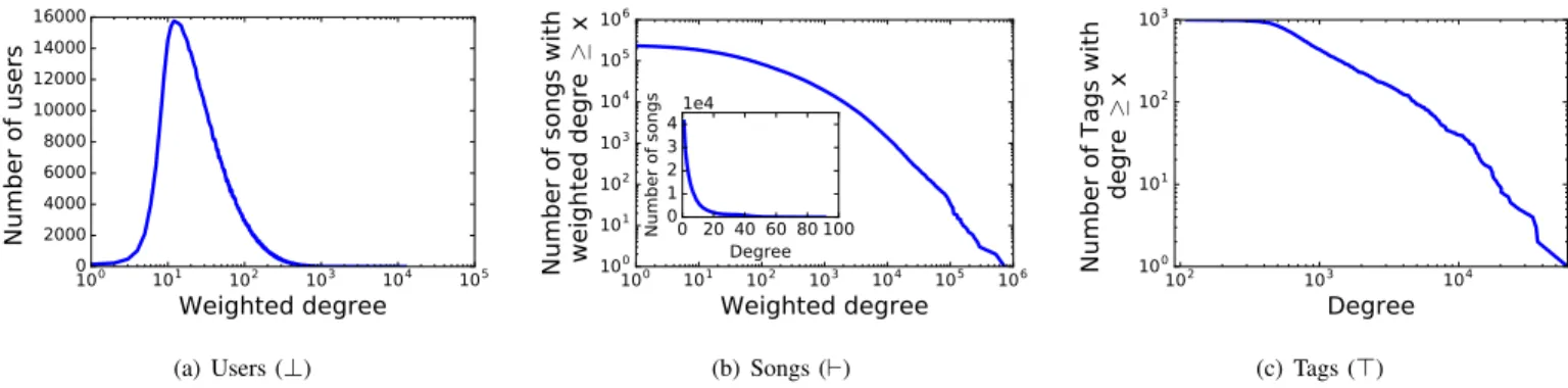
In addition to the information on the size presented above, we show in Figure 3 the distribution of the links in the tripartite graph.
Figure 3(a) presents the distribution of the weighted degree for the users. Although the complete range of values and is high (the x-axis is in log scale) as well as the maximal value (12 387), the order of magnitude remains quite homogeneous for all users: a user listens 105 times to a song and listens to 37 different songs in average and those values are quite representative of a random user.
Figure 3(b) presents the distribution of the degrees for the songs both towards the users (cumulative weighted degree distribution, in log-log scale) and towards the tags (inset, degree distribution in linear scale). The plot shows that the popularity of the songs is very heterogeneous. Some song are highly popular (listened to more than 100 000 times) while the vast majority of songs have a small number of play counts (91% songs are listened to less than 1 000, 64% less than 100 times) and a little audience (78% of the songs are listened to by less that 100 different users).
3we removed tracks known to be matched to wrong songs, see https://
labrosa.ee.columbia.edu/millionsong/blog/12-2-12-fixing-matching-errors.
4some tags, such as ”rock” or ”metal”, clearly describe musical content
100 101 102 103 104 105
Weighted degree
0 2000 4000 6000 8000 10000 12000 14000 16000Number of users
(a) Users (⊥) 100 101 102 103 104 105 106Weighted degree
100 101 102 103 104 105 106Number of songs with w
eig
ht
ed
d
eg
re
≥x
0 20 40 60 80 100 Degree 0 1 2 3 4 Number of songs 1e4 (b) Songs (`) 102 103 104Degree
100 101 102 103Number of Tags with
d
eg
re
≥x
(c) Tags (>) Fig. 3. Degree distributions in the tripartite graph.In regards to the links towards the tags (inset of Figure 3(b)), a lot of songs have a very small degree. In particular, 72% of the songs have less than 10 tags among the 1000 possible. This is expected as the tags are meant to describe the content and feeling related to a song which induces naturally a small number of possible combinations.
Finally, Figure 3(c) presents the inverse cumulative distribu-tion of the tag’s toward the songs. The plot (in log-log scale) exhibits clearly an heterogeneous distribution of the use of the tags. Similarly to the song’s play count, some tags are extremely popular while a majority of tags are used a small number of times by the users.
All in all, the present dataset exhibits properties usually observed in similar systems. In particular, the popularity of the songs are highly heterogeneous and the behaviour of a random users is regular.
Before turning to the analysis of the diversity, let us recall that the bipartite projection of the studied structure allows to study how users are related to tags. In the context of this dataset, we will use the term of volume to refer to the weighted degree of the links in the projection. Thus the volume of a tag t is defined as the sum of the number of play counts for all songs with tag t. Similarly, the volume of listening of a user u is the sum of the number of tags for all songs listened to by u and multiplied by their play count. We will just use the term ”volume” when there is no ambiguity.
We turn now to the results. We start by showing how the proposed herfindahl diversity can be used to study the diversity of the audience captured by a category (Section IV) before turning to the study of the diversity of users attention (Section V).
IV. DIVERSITY OF THE TAGS AUDIENCE
Fig. 4 shows the distribution of the diversity for all the 1 000 tags. This distribution is very heterogeneous, with an average value of 9 699 (and median of 5 111) but exhibiting some tags with a particularly high diversity (higher than 100 000). This shows that tags may have a very different public, ranging from a very broad audience to very narrowed ones.
0.0 0.2 0.4 0.6 0.8 1.0 1.2
Herfindahl diversity
1e50 20 40 60 80 100 120 140 160 180
Number of tags
0.0 0.2 0.4 0.6 0.8 1.0 1e4 0 20 40 60 80 100 Zoom (0 to 10 000)Fig. 4. Distribution of the diversity of the tags audience.
Focusing on the latter (see inset on Figure 4), one can see however that tags with a diversity score lower than 10 000 (which represents 75% of the tags) shows a more homogeneous diversity value, centered around 5 000.
This diversity suggests to investigate more in depth how the score behave according to the tags and in particular whether it can discriminate between different tags audience. In order to investigate this question, and because manual analysis of 1 000 tags is out of reach, we focus now on a selection of 25 tags.
A. A focus on 25 tags
Even among the 1 000 most popular tags, different sorts of tags appear. This is due to the fact that different users have very different ways to use tags to describe the content of a song. Some tags are for instance clearly used to describe the type of music related to a song (like ”rock”, ”metal” or ”country”). We will refer to those tags as musical tags and represent them with plain blue markers on Figures.
In contrast, others tags relate less to the content of a song than its context: for instance the emotion felt when listening to the song (”awesome”, ”best”), the period at which the song was created (”1986”, ”70s”) or even why or when it is listened to (”tosleep”, ”shower”). We will refer to those tags as generic tags in the following and depict them with red
rock pop poprock hardrock hiphop
folk
metal punk rnb rap
punkrock country alternative favorites love indie dance chill loved indiepop epic good sweet slow best
Tags
0.0 0.2 0.4 0.6 0.8 1.0 1.2Herfindahl diversity
1e5(a) Diversity of tags audience
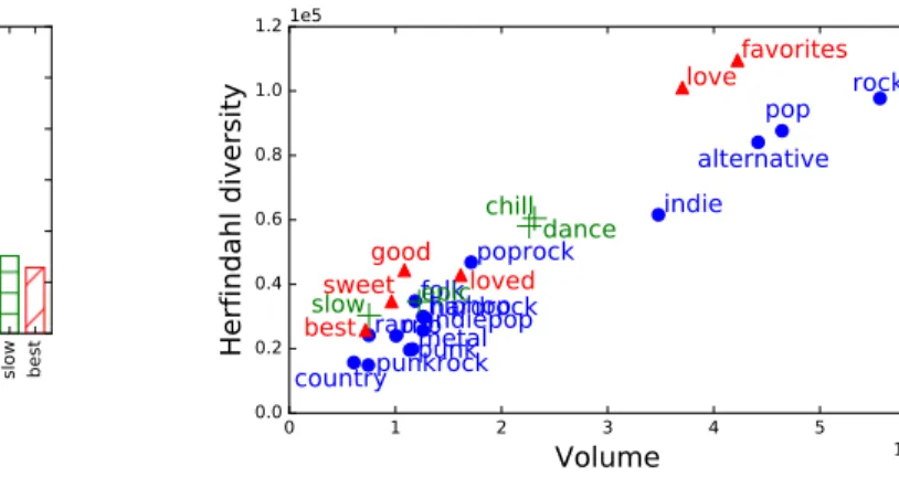
0 1 2 3 4 5 6 Volume 1e7 0.0 0.2 0.4 0.6 0.8 1.0 1.2 Herfindahl diversity 1e5 rock pop poprock hardrock hiphop folk metal punk rnb rap punkrock country alternative indie indiepop dance chill epic slow favorites love loved good sweet best
(b) Diversity of tags audience according to their volume Fig. 5. Analysis of the diversity of a selection of 25 tags.
triangles (or red dash lines).
Sometimes, a tag can also be a mix of the two precedent categories, mainly because of its polysemy. For instance, chill clearly refers to an emotion but is also more and more used to refer to a type of music. We will refer to those tags as mix tagsin the following and use green cross markers.
This distinction is interesting to notice since one can expect the herfindahl diversity to be able to discriminate between musical and generic tags. The former leading naturally to a more narrowed audience than the latter, its diversity is likely to be lower.
In order to investigate this question, we selected manually 25 among the 50 most popular tags: 15 are musical tags, 6 are generic tags and 4 are mix tags. Although this selection is completely subjective, we tried to have representatives from each category and tags with volumes allowing comparison. The list is provided in Figure 5 with the herfindahl diversity of each tag.
Surprisingly one can observe on Figure 5(a) that highly diverse tags appear in the two extreme categories: ”rock”, ”pop” and ”alternative” for musical tags; ”favorites” and ”love” for generic ones. Similarly, tags with a low diversity can be observed in every categories: ”country” and ”metal” for musical tags; ”best” for generic ones and ”slow” for mix ones.
This observation raises some doubts about what the herfind-ahl diversity actually captures. It is quite surprising that tags like ”favorites” and ”best” for instance have such a different diversity although they are likely to be synonymous in this context.
Investigating those tags in particular, it turned out that the diversity score of a tag is highly correlated to the volume of its audience (i.e. the number of times songs of its category have been listen to, see Section III-B). The highest its audience, the highest its diversity. This can be clearly observed in Figure 5(b). This raises the question of compensating the effect of the volume in order for the score to capture precisely the diversity instead of its volume. This is what the next section
is devoted to.
B. Calibrated herfindahl diversity
In network science, one classical way to take into account the effect of a property on a score is to compare this score to what is its expected value for random networks with a similar property. This is usually done using models that generate random networks respecting the property of interest.
In our context, we used a variant of the configuration model [16] which randomly assigns edges to match a given degree sequence without adding any other expected property. We used it to shuffle the bottom part of the tripartite structure in order to reassign randomly the links between the users and the songs.
More precisely, we generated tripartite graphs having the same number of nodes and links but such that the links of E⊥
T (with their weight) are distributed uniformly at random
among ⊥ and ` nodes according to their observed degree. The other links (i.e. between ` and >) are kept unchanged.
This means that, compared to the original, the songs of the generated tripartite graphs have the exact same tags and are listened to the same number of times but by random users. Similarly, every user listens to the same number of songs but those songs are selected uniformly at random.
Doing so, one can generate several random tripartite graphs and compute what is the average herfindahl diversity for every tag. This average value is then used to divide the herfindahl diversity which results in the calibrated herfindahl diversity. Formally, let Rand(T) be the random tripartite graph generated from T by the model, the calibrated herfindahl diversity of u in T is defined by:
chd(T, u) = hd(T, u) hd(Rand(T), u)
It is worth noticing here that the volume of a tag in the original and in the generated tripartite graphs is the same. This allows for a fair comparison between the two values,
0 1 2 3 4 5 6 Volume 1e7 0.05 0.10 0.15 0.20 0.25 0.30 0.35 0.40 Calibrated herfindahl diversity rock pop poprock hardrock hiphop folk metal punk rnb rap punkrock country alternative indie indiepop dance chill epic slow favorites love loved good sweet best
Fig. 6. Calibrated diversity of tags audience according to their volume
hence legitimating the definition of the calibrated herfindahl diversity.
The result is shown in Figure 6. As expected, the compar-ison with the random model compensates for the impact of the volume on the way diversity is computed. No particular correlation can now be observed between volume and cali-brated herfindahl diversity. This does not prevent tags with high volume to still have a relatively high diversity, since they have a better chance to reach a broader audience. One can see in particular that the diversity slightly increases with the volume.
Besides, the calibrated diversity seems to restore balance between tags very close on the semantic level while very contrasted in terms of use. The tags love and loved for instance exhibit now a similar diversity (around 0.29) although they have a very different volume (love is almost 4 times more used than loved). Similar observations can be drawn for the tags indie and indiepop.
In addition, the plot shows now that the calibrated herfindahl diversity can discriminate between generic tags (upper part of the plot) and musical tags (mostly in the bottom part): generic and mix tags all have a high diversity (between 0.23 and 0.35) while musical tags tend to have a lower value (from 0.09 to 0.22).
The only exception is poprock that has a relatively high diversity for a musical tag (0.27) and despite its low volume (17M total play counts). Although it is difficult to draw a conclusion from this value only, one can speculate on the fact that the tags rock and pop taken independently also have a high diversity. This might explain why poprock builds on their success and reaches a broader and more diverse audience.
Finally, the fact that the calibrated diversity is now inde-pendent from the volume allows for comparisons of musics with similar volume. For instance, one can spot that, although they all have a similar audience size (around 10M total play counts), rap and rnb touch a way more diverse public than metal and punk, that seem to be confined to a more narrowed public. 0 50 100 150 200 250
Herfindahl diversity
0.0 0.2 0.4 0.6 0.8 1.0 1.2Number of users
1e4Fig. 7. Distribution of the diversity of users attention.
V. DIVERSITY OF THE USERS ATTENTION
We turn now to the analysis of the diversity of users attention. Formally, the approach is similar to the one used in the previous section except that the random walks start from ⊥ nodes instead of > nodes.
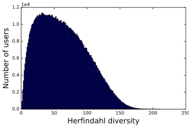
Figure 7 shows the distribution of the herfindahl diversity of all users attention. The plot, in lin-lin scale, shows clearly a homogeneous distribution, well centered around average values (the mean is 63, median is 59) even if one can observe some users with a particularly high diversity of attention. This is in line with the distribution of users volume (Section III-B) and manual investigations revealed that most of those highly diverse users correspond to the outliers observed in Figure 3(a).
In addition to the distribution of diversity, the previous section focused more precisely on 25 tags to study whether the introduced metric could discriminate between different be-haviours. Unfortunately, due to the anonymization processes, we have no information on the users5. Therefore, we cannot
relate the herfindahl diversity to external explanations similarly to what we did with the tags at the semantic level.
However, one can study how the diversity of a user attention is related to its volume. Indeed, while one can expect the diversity to be correlated to the volume, it is not clear how the correlation operates.
Figure 8 provides some elements to investigate this question. In particular, Figure 8(a) displays the distribution of the volume of the user (i.e. the number of tags for all songs listened to by the user and multiplied by their play counts). Although the x-axis is in log-scale, one can see that the order of magnitude is homogeneous in the network. The vast majority of the users (87%) have a volume between 10 and 2 000.
This gives enough elements to study how the diversity of a user attention evolves as its volume grows. Figure 8(b)
100 101 102 103 104 105
Volume
0 200 400 600 800 1000 1200 1400Number of users
(a) Distribution of users volume
0 500 1000 1500 2000
Volume
0 20 40 60 80 100 120 140 160Herfindahl diversity
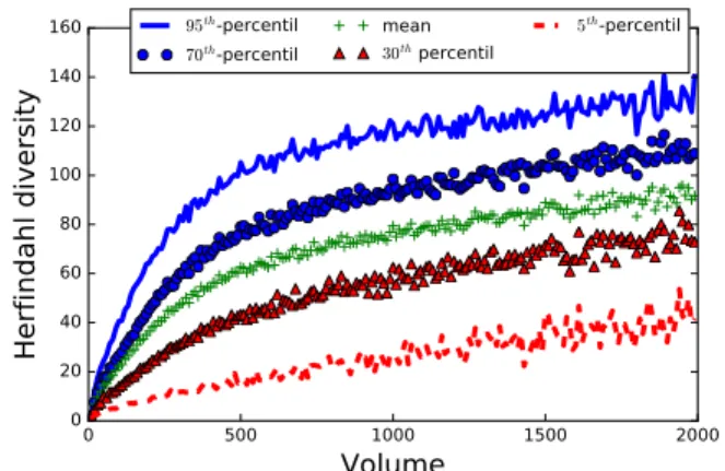
95th-percentil 70th-percentil mean 30th percentil 5th-percentil(b) Diversity of users attention according to their volume Fig. 8. Analysis of users attention.
depicts such evolution for volumes less or equal to 2 000 6.
For each volume, the plot shows what is the mean herfindahl diversity observed, along with the 5th, 30th, 70thand the 95th
percentile.
One can see that the influence of the volume on the diversity operates in two phases. Between volume 0 and 500, the progression is sharp, in particular for the upper part of the population (mean and above) while the progression is slower for higher volumes.
This indicates some sort of saturation in the diversity of users attention: as the volume of listening reaches a certain threshold (around 500 in our observations), an average user starts to listen repeatedly to similar musical contents (approx-imated by the tags) and the diversity tends to increase more slowly.
The redundancy observed in the listening of the users explains why the average diversity (63) is far from the maximal theoretical value (1 000 in our dataset). Although the volume tends to widen the musical perspective of a user, its taste towards a limited amount of different contents limits its musical diversity.
VI. CONCLUSION&PERSPECTIVES
In this paper, we investigated the question of quantifying the diversity in users activity. We proposed to represent this activity as a tripartite graph relating users to products and products to categories. Then we defined the herfindahl diver-sity as a way to quantify the extent to which the distribution of probabilities obtained from a random walk on this structure is close to a uniform distribution.
We applied this approach on a dataset recording the activity of users on online music platforms. In this dataset, a user listens to songs that are tagged. Thanks to this structure, we were able compute the herfindahl diversity on random walks issues either from users or from tags. We get respectively the diversity of the users attention and the one of the tags audience.
6for higher values, we had too few users to have confidence on the
observations
The results are twofold. First, analyzing the tags audience, we showed how to compensate from the effect of the volume on the diversity and defined the calibrated herfindahl diversity. This second score turned out to be a good indicator to discriminate between musical tags (low diversity) and generic tags (high diversity), independently from their volume.
Second, focusing on users attention, we studied the relation between the volume and the diversity. It revealed a saturation phenomenon: while the growth of the diversity is initially high as the volume increase, this progression slows down after a certain threshold, indicating that when the volume is too high, users tend to listen repeatedly to similar musical contents.
All the analysis proposed in this study relies on choices made to capture the notion of diversity. Several elements might have been done differently and we discuss below possible variants and extensions.
A. Generalizing diversity indexes
Given a distribution of probabilities P = (pi)i issued from
a random walk, we proposed in this paper to rely on an adaptation of the herfindahl index to quantify the extent to which the distribution is close to a uniform distribution, hence a maximal diversity. Other choices might have been done by relying on other indexes. In particular:
Richness div0(P ) = Pi1pi>0 Shannon div1(P ) = 2− P ipilog(pi) Herfindahl div2(P ) = (Pip 2 i)−1
Berger-Parker div∞(P ) = (maxi(pi))−1
Moreover, those 4 indicators can be unified with the follow-ing definition of a diversity function div:
divα(P ) = ( X i pαi) 1 (1−α)
where α is now a parameter of the level of diversity one wants to capture. In this paper, we used exactly this diversity function with α = 2.
In order to ease the explanation that follows, we will focus on the interpretation of those indicators when applied on random walks issued from users (⊥ nodes), i.e. when analyzing the diversity of users attention (see Section V).
In this context, when α = 0 (Richness) one simply counts the number of categories that a random walk reaches, without considering its distribution. On the contrary, when α = ∞ (Berger-Parker) one only considers the value of the category that has the highest probability of being reached, without considering the other categories.
Intuitively, those two indicators constitute the two dimen-sions one wants to capture in a diversity index: the number of categories reached and their distribution. In that regard, when α = 1 (Shannon7, widely used in information theory)
or α = 2 (Herfindahl, mostly used in economy and social sciences), one succeeds in providing a more nuanced point of view by accounting for those two dimensions.
It is worth noting that, just as the herfindahl diversity used in this article, those indicators are all bounded by the number of categories reached by the random walks (which is exactly the value of the richness) and that, for α ≥ 1, this maximum value is reached when the distribution is uniform.
This provides a unified framework within which one can explore the different facets of diversity. We plan to investigate the behaviour of the diversity function with various α in the future.
B. Impact of random models.
A second choice has been made when trying to compensate for the impact of the volume in the herfindahl diversity. Following the classical approach, we compared the score of the diversity to what it would have been in a similar random structure. In this approach, everything relies on the notion similar random structure. The choice we made was to shuffled the links between the bottom and middle layer of the tripartite graph (i.e. between the users and the songs) while keeping the rest unchanged.
This choice was motivated by the fact the volumes of the tags are kept unchanged in the process, thus legitimating the comparison of the values. However, one could have proposed several other ways to disturb the structure.
For instance, one might relax some constraints and random-ize also the links between the songs and the tags. Another parameter could be to randomize the weights attached to the links. All those choices would have resulted in different scores and we plan to investigate those variants in the near future in order to better understand what is their impact on our perception of diversity.
Besides, instead of relying on random generations, we intend to develop analytical results expressing formally the expected diversityfor different random models and for various value of α. This would strengthen the results obtained with the calibrated version of the diversity.
7more formally, for α → 1, div
α(P ) tends to Shannon.
ACKNOWLEDGMENT
This work is funded in part by the European Commission H2020 FETPROACT 2016-2017 program under grant 732942 (ODYCCEUS), by the ANR (French National Agency of Research) under grants ANR-15-CE38-0001 (AlgoDiv), by the Ile-de-France Region and its program FUI21 under grant 16010629 (iTRAC).
REFERENCES
[1] A. Jeckmans, M. Beye, Z. Erkin, P. Hartel, R. Lagendijk, and Q. Tang, “Privacy in recommender systems,” in Social Media Retrieval, ser. Computer Communications and Networks, N. Ramzan, R. van Zwol, J.-S. Lee, K. Cl¨uver, and X.-S. Hua, Eds. Springer Verlag, 2013, pp. 263–281.
[2] R. Epstein and R. E. Robertson, “The search engine manipulation effect (seme) and its possible impact on the outcomes of elections,” Proceedings of the National Academy of Sciences, vol. 112, no. 33, pp. E4512–E4521, 2015. [Online]. Available: http://www.pnas.org/content/ 112/33/E4512
[3] L. Gu, V. Kropotov, and F. Yarochkin, “The fake news machine: How propagandists abuse the internet and manipulate the public,” Trend Micro, Tech. Rep., 2017. [On-line]. Available: https://documents.trendmicro.com/assets/white papers/ wp-fake-news-machine-how-propagandists-abuse-the-internet.pdf [4] E. Bakshy, S. Messing, and L. A. Adamic, “Exposure to ideologically
diverse news and opinion on facebook,” Science, vol. 348, no. 6239, pp. 1130–1132, 2015. [Online]. Available: http://science.sciencemag. org/content/348/6239/1130
[5] F. Pasquale, The Black Box Society: The Secret Algorithms That Control Money and Information. Cambridge, MA, USA: Harvard University Press, 2015.
[6] D. Beer, “The social power of algorithms,” Information, Communication & Society, vol. 20, no. 1, pp. 1–13, 2017.
[7] B. Goodman and S. Flaxman, “Eu regulations on algorithmic decision-making and a ”right to explanation”,” 2016, cite arxiv:1606.08813Comment: presented at 2016 ICML Workshop on Human Interpretability in Machine Learning (WHI 2016), New York, NY. [Online]. Available: http://arxiv.org/abs/1606.08813
[8] E. Bozdag, “Bias in algorithmic filtering and personalization,” Ethics and Inf. Technol., vol. 15, no. 3, pp. 209–227, Sep. 2013. [Online]. Available: http://dx.doi.org/10.1007/s10676-013-9321-6
[9] C.-N. Ziegler, S. M. McNee, J. A. Konstan, and G. Lausen, “Improving recommendation lists through topic diversification,” in WWW ’05: Proceedings of the 14th international conference on World Wide Web. New York, NY, USA: ACM, 2005, pp. 22–32. [Online]. Available: http://portal.acm.org/citation.cfm?id=1060754
[10] T. Zhou, Z. Kuscsik, J.-G. Liu, M. Medo, J. R. Wakeling, and Y.-C. Zhang, “Solving the apparent diversity-accuracy dilemma of recommender systems,” Proceedings of the National Academy of Sciences, vol. 107, no. 10, pp. 4511–4515, 2010. [Online]. Available: http://www.pnas.org/content/107/10/4511
[11] G. Adomavicius and Y. Kwon, “Improving aggregate recommendation diversity using ranking-based techniques,” IEEE Trans. on Knowl. and Data Eng., vol. 24, no. 5, pp. 896–911, May 2012. [Online]. Available: http://dx.doi.org/10.1109/TKDE.2011.15
[12] P. Resnick, R. K. Garrett, T. Kriplean, S. A. Munson, and N. J. Stroud, “Bursting your (filter) bubble: Strategies for promoting diverse exposure,” in Proceedings of the 2013 Conference on Computer Supported Cooperative Work Companion, ser. CSCW ’13. New York, NY, USA: ACM, 2013, pp. 95–100. [Online]. Available: http://doi.acm.org/10.1145/2441955.2441981
[13] W. F. Stolper, “National power and the structure of foreign trade. albert o. hirschman,” Journal of Political Economy, vol. 54, no. 6, pp. 562–563, 1946.
[14] A. Hirschman, “The paternity of an index,” The American economic review, vol. 54, no. 5, pp. 761–762, 1964.
[15] T. Bertin-Mahieux, D. P. Ellis, B. Whitman, and P. Lamere, “The million song dataset,” in Proceedings of the 12th International Conference on Music Information Retrieval (ISMIR 2011), 2011.
[16] M. E. Newman, “The structure and function of complex networks,” SIAM review, vol. 45, no. 2, pp. 167–256, 2003.