Body coupled communication : the channel and implementation

Body Coupled Communication: The Channel and

Implementation

by

OF

Grant Seaman Anderson

_JU

B.S., University of Utah (2009)

M.S., University of Utah (2009)

Submitted to the Department of Electrical Engineering and Computer

Science in partial fulfillment of the requirements for the degree of

Doctor of Philosophy

at the

MASSACHUSETTS INSTITUTE OF TECHNOLOGY

June 2017

Massachusetts Institute of Technology 2017. All rights reserved.

Author ...

Certified by.

N 23 2017

BRARIES

ARCHIVES

... ....

...

...

Department of Electrical Engineering and Computer Science

March 31, 2017

. . . ....

. ...

.

. . . ..

Charles G. Sodini

LeBel Professor of Electrical Engineering

Thesis Supervisor

Accepted by...

...

...

Leslie A. Kolodziejski

Professor of Electrical Engineering and Computer Science

Chair, Department Committee on Graduate Students

Body Coupled Communication: The Channel and

Implementation

by

MAss

Grant Seaman Anderson

_JU

B.S., University of Utah (2009)

_I

M.S., University of Utah (2009)

Submitted to the Department of Electrical Engineering and Computer

Science in partial fulfillment of the requirements for the degree of

Doctor of Philosophy

at the

MASSACHUSETTS INSTITUTE OF TECHNOLOGY

June 2017

Massachusetts Institute of Technology 2017. All rights reserved.

Author ...

Certified by .

Accepted by...

N 23 2017

3RARIES

ARCHIVES

Signature redacted

Department of Electrical Engineering and Computer Science

March 31, 2017

Signature redacted

Charles G. Sodini

LeBel Professor of Electrical Engineering

Thesis Supervisor

Signature redacted

...

...

6(1

Leslie A. Kolodziejski

Professor of Electrical Engineering and Computer Science

Chair, Department Committee on Graduate Students

Body Coupled Communication: The Channel and Implementation

by

Grant Seaman Anderson

B.S., University of Utah (2009)

M.S., University of Utah (2009)

Submitted to the Department of Electrical Engineering and Computer Science on March 31, 2017, in partial fulfillment of the

requirements for the degree of Doctor of Philosophy

Abstract

To achieve comfortable form factors for wearable wireless medical devices, battery size, and thus power consumption, must be curtailed. Often the largest power consumption for wireless medical devices is storing or transmitting acquired data. Body area networks (BAN) can alleviate power budgets by using low power transmitters to send data locally around the body to receivers that are on areas of the body that allow for larger form fac-tors, like the wrist or the waist. Body coupled communication (BCC) has been shown to have great potential in forming a BAN. This work expands the potential of BCC BANs by showing that BCC can include implanted nodes. Implants being able to implement BCC is an impactful discovery as previous BCC channel models have implicitly stated that BCC cannot work with implants. This discovery will allow BANs that include implants, such as pacemakers, to utilize the power efficiency of BCC.

This thesis will give an introduction to BANs and BCC. It will further detail three con-tributions to BCC and its implementation. The three concon-tributions are: 1) an excellent understanding of the BCC channel, that is verified by careful measurements, 2) a new am-plifier circuit that improves the signal to interferer ratio, and 3) an asynchronous digital communication scheme that offers a high data rate and low power implementation. An integrated transmitter and receiver were fabricated in a 0.18 pm CMOS process. The re-sults of the three contributions as implemented in the integrated chips are also presented and discussed. The integrated receiver was able to receive information at 16 Mbps, while consuming 5.9 mW, yielding an energy use of 367 pJ/bit. The integrated transmitter was able to transmit information at 30 Mbps, while consuming 4.32 mW, yielding an energy

use of 114 pJ/bit.

Thesis Supervisor: Charles G. Sodini

Acknowledgments

I would like to thank my wife. Her encouragement has helped me finish my PhD and her support has made it possible. We have been married two years now and it still surprises me how well she can make me laugh. One such instance was her desire for me to not write anything in this acknowledgments section and just have "This Page Intentionally Left Blank" written in the middle. We are excited to meet our daughter this September.

I also want to acknowledge my adviser Charlie. He has supported me in life. When my mother passed away in 2014 he said take as much time as you need. He encouraged me to get married, take vacations, and enjoy graduate school. He has helped me to learn the correct questions to ask in research and shown me how to approach problems and tackle them. I appreciate that with Charlie I have never questioned that his priority was to help me excel, and that he had my best interest at heart.

I want to thank Jeff Lang for his help in the body model of BCC and his willingness to meet with me and get into the details with me.

Muriel Medard was also very helpful and willing to meet with me to discuss asyn-chronous communication and it's ramifications.

Contents

1 Motivation and Background ₁₇

1.1 Body Area Networks . . . . 17

1.2 _{Use Models for BCC . . . 21}

1.3 Contributions . . . 22

2 Introduction to Body Coupled Communication 23 2.1 _{Measuring BCC Channel . . . 27}

2.1.1 Channel Measurment Equipment . . . 28

2.1.2 Electrodes used for Measurements . . . 32

2.2 _{Return Path . . . 34}

2.2.1 _{Measurments to Determine Dominant Current Path . . . 38}

2.3 _{Body Model . . . 45}

2.3.1 _{The Physical Theory . . . 45}

2.3.2 Spreading Resistance . . . 52

2.4 _{Proposed BCC Channel Model . . . 54}

2.4.1 _{Implantable Channel . . . 56}

2.4.2 Implications of the Proposed Channel . . . 57

2.5 _{Summary . . . 59}

3 Optimizing the Receiver for BCC: Body Buffered Return 61 3.1 Optimizing the Receiver for BCC . . . . 61

3.2 _{Body Buffered Return . . . 63}

3.3 Validation of BBR . . . .

3.3.1 BBR Using a Source-Follower MOSFET . . . .

3.4 Summary . . . .

4 Asynchronous Digital Communication

4.1 Synchronous Digital Communication . . . .

4.2 _{Asynchronous Digital Communication . . . .}

4.3 Implementation of Asynchronous Digital Communication. 4.3.1 Start U p . . . . 4.3.2 Optimizing Data Rate . . . .

4.4 Symbol Transitions . . . .

4.5 Baud Error Rate & Bit Error Rate . . . . 4.6 Summary . . . .

5 Integrated Asynchronous Transmitter and Receiver

5.1 Transmitter . . . .

5.1.1 Transmitter Results . . . .

5.2 R eceiver . . . .

5.2.1 Frequency Detection . . . .

5.2.2 Frequency Detection using Counting . . . .

5.2.3 _{Integrated Circuit Counter . . . .}

5.2.4 _{Analog Front End . . . .}

5.2.5 Full Integrated Receiver . . . .

5.2.6 Receiver Measured Results . . . .

5.3 Transmitter and Receiver Performance Comparison . .

5.4 Summary . . . .

79

95

. . . 95

6 Conclusion

6.1 This W ork's Impact .. .... .. .. .. . .. .. .. .. .. . .. ..

117 119 71

74

List of Figures

1-1 Body area network diagram. There are various ways to implement body area networks including eTextiles, radio, and BCC. . . . . 19 1-2 Energy efficiency of UWB and NB radio, and BCC transceivers as found

in [3 ]. . . . . 20 2-1 The BCC channel. The electrodes on the transmitter and receiver form

capacitive links A-K. . . . 24

2-2 The circuit diagram from figure 2-1 where the color of the capacitor plates are color coded with black to be electrodes, green the environment, and peach the body. The resistor is the input impedance of the receiver. . . . . . 24 2-3 Traditional BCC circuit diagram. . . . 26

2-4 Using equipment that shares a common node will significantly change the current paths in BCC, resulting in inaccurate measurements. . . . . 27 2-5 Both grounded equipment and discrete battery powered boards were used

to measure the gain in the channel. The comparison of the two measure-ments show contrasting channel gains. . . . . 28 2-6 Functional schematic of the transmitter. . . . . 29 2-7 Functional schematic of the receiver. . . . . 29 2-8 The full test configuration to measure the BCC channel. The BCC channel

is measured as the output of the transmiter, and input of the receiver. The channel includes all four capacitive links. . . . . 31 2-9 While there is a resistive element to the BCC link, the link is dominated by

2-10 Two possibilities for the dominant current path; the dominant current path is shown with the blue loop. (a) The dominant current path as through both the body and the environment. (b) The dominant current path as solely

through the body. . . . 35

2-11 The differences in the ideal electrode placement for the environmental re-turn verse the body rere-turn. (a) depicts how the transmitter's/receiver's elec-trodes should be placed if the dominant current path is through the environ-ment: one electrode as close to the body as possible, and the other as far away as possible. While (b) depicts how the electrodes should be placed if the dominant current path is through the body: both electrodes are as close to the body as possible. . . . . 37 2-12 The channel gain as a function of the distance between an electrode and

the body; normalized when the electrode is attached directly to the body. The bottom horizontal lines are the channel gain when the electrode was disconnected from the receiver. . . . . 39 13 A circuit model to give a possible explanation of the inflection in figure

2-12. The voltage source, Vn, models the transmitter, the capacitors attached to the transmitter represent the capacitive links made by the electrodes and body, and one of the electrodes and environment (see figure 2-10), the three resistors (making the pi-network) model some fixed attenuation due to the body, while the resistor between Vo₀ and ground model the input resis-tance of the receiver. . . . . 40 2-14 Simulated results from the circuit diagrammed in figure 2-13. . . . . 42

2-15 On the left, of both (a) and (b), is a transmitter using two electrodes to

couple to the body. A receiver is coupling to the same body with electrodes some distance away. (a) Both of the transmitter's electrodes are close to the body. (b) By moving an electrode farther away from the body, the fringe capacitance made by this electrode couples to areas on the body that are closer to the receiver's electrodes. . . . . 43

2-16 The channel gain as a function of the distance between an electrode and the pork loin; normalized when the electrode is attached directly to the pork loin. 44 2-17 A cross section of hemispherical electrodes placed into a medium. The

medium is infinite along five directions, and bounded by an infinite plane on the sixth. . . . 46 2-18 Hemispherical electrode placed into an infinite medium. . . . . 47 2-19 The current injected into the medium will produce a uniform current density. 48 2-20 The voltage difference between the electrode and the point 'P'. . . . . 48 2-21 An aerial view of four Hemispherical electrodes placed on the medium's

surface. . . . . 50

2-22 The body can be modeled as a lattice work of impedances. Different types of tissues will have different impedances and there will be transition impedances between different tissues. . . . . 52

2-23 The detailed model of the impedances in Figure 2-22. . . . 53 2-24 The circuit model for the BCC channel, with the body modeled as a

spread-ing resistance. Validated for frequencies from 10 MHz - 150 MHz. . . . . . 53 2-25 The proposed BCC channel model. The body is modeled as a spreading

resistance. This model is valid from 10 MHz - 150 MHz . . . . 54 2-26 BCC channel measurements with the input resistance to the receiver varied. 55 2-27 (a) The proposed BCC channel model when both transmitter and receiver

are connected by capacitive links to the body. (b) The proposed BCC chan-nel model when the transmitter is an implant in the body that is galvani-cally connected to the BCC channel, and the receiver is outside the body connected to the channel by the capacitive links. . . . . 57 2-28 The channel gain measurements showing the difference between an

exter-nal transmitter, that is capacitively coupled, and an implanted transmitter that is galvanically coupled . . . . 58 3-1 The receiver is connected with its local ground being coupled back through

3-2 The receiver is connected with the output of a buffer being coupled back

through the body. . . . 62

3-3 The thevenin equivalent of the transmitter and the BCC channel. . . . . 63

3-4 The amplifier connected in the traditional way . . . . . 64

3-5 The amplifier connected in the BBR configuration. . . . . 65

3-6 Interferers can also couple to the electrodes. (a) shows an interferer cou-pling to the traditional amplifier, and (b) shows an interferer coucou-pling to a BBR amplifier. Such interferes could be other devices polluting the spec-trum, or even the gained up signal of the receiver coupling back to its own input. BBR can provide a higher signal to interferer ratio. . . . 67

3-7 Applying BBR to a differential amplifier. (a) A standard differential ampli-fier. (b) By removing the impedances Z1 and Z2 from (a) a virtual short is created between the electrodes, making this a differential BBR amplfier. . . 69

3-8 A fully differential amplifier topology connected in the BBR configuration. Notice the amplifier creates a virtual short between the two electrodes. . . . 70

3-9 The magnitude frequency response for BCC channel using BBR. . . . . 72

3-10 The magnitude frequency response for BCC channel, comparing both tra-ditional and BBR. . . . 73

3-11 An nMOS source-follower. . . . . 74

3-12 The testing circuit for the nMOS source-follower. . . . . 75

3-13 (a) BBR using a source-follower. (b) Zoomed in to see detail.. . . . . 77

4-1 Frequencies/symbols being interpreted with different clocks. Each clock validates a frequency/symbol on its rising edge. Clocks 1 and 2 are the same frequency but with different phase, while clock 3 is a different fre-quency. ... ... 81

4-2 One way to define the codeword relationship between three frequency tran-sition s. . . . . 83

4-3 Sent codewords, as a function of the frequency changing. The codeword relationship between frequencies used are found in figure 4-2. . . . . 84

4-4 Sending the bit stream '100 000 000 111' with 3-bit asynchronous

dig-ital communication. The yellow-colored symbol identifies the frequency

before the hop, while the blue designates the frequency after the hop. . . . . 85

4-5 The signal path for an asynchronous digital communication receiver. . . . . 86

4-6 An AFSK scheme with an arbitrary code-word relationship between the 3 sym bols/frequencies. . . . 90

4-7 An AFSK scheme with the code-word relationship between the 3 sym-bols/frequencies optimized to send the codeword '0' quickly. . . . . 90

4-8 The three valid voltage levels of an AASK scheme. . . . 92

4-9 If a transmitter transitions from V to V2, it will have to slew through V1. If the slewing voltage is in the region that will be recognized as V long enough to be detected by the receiver, a symbol transition error will occur. 92 5-1 The block diagram of the AFSK transmitter. . . . 96

5-2 The transmitter sending every possible transition. The pattern that was sent was n0n1n20n01021n10122n2021, _where 'n' _{is no frequency and 0 is FO etc. 98} 5-3 _{The block diagram of the AFSK receiver. . . . 101}

5-4 Three ways in which to detect a frequency. 1) Passive Filter 2) FFT/Digital Filter/Corrilation Filter 3) Counting . . . 102

5-5 Possible counts when the counter's period is not a factor of the count period. 104 5-6 Possible counts when the counter's period is not a factor of the count period. 105 5-7 _{Block diagram of integrated counter. . . . 106}

5-8 Receiver's analog front end. _{. . . 107}

5-9 Common source amplifier as used in receiver's LNA. . . . 108

5-10 The full integrated receiver's block diagram. . . . 109

5-11 The output of the frequency divider (black), will be a 50% duty cycle at 1/2 the frequency of the input. . . . . 110

5-12 Diagram of when the receiver detects a valid frequency. There are two count registers, one stores the count when the input frequency was high (green) and one when it was low (blue). The clock's rising edge increments the counter during the respective phase. When both count registers corre-late with the same frequency as found in section 5.2.3, the corresponding

'frequency detected' line will be brought high. . . . .111 5-13 The BaudER for the AFSK receiver. . . . 113 5-14 This work's transmitter and receiver performance (the respective stars) as

List of Tables

4.1 Communication Definitions and Examples . . . 80

5.1 Transmitter Power Consumed for a Data Rate of 30 Mbps . . . 99

5.2 Transmitter FOM for a Data Rate of 30 Mbps . . . 100

5.3 _{BCC Integrated Receiver Performance . . . 112}

Chapter 1

Motivation and Background

Biological signals, such as the electrocardiogram (ECG) and electroencephalogram (EEG), are often recorded in areas of the human body where attaching sensors with large form fac-tors would not be comfortable and therefore are not compatible with long-term recording. Making sensors with small form factors places limits on battery size, requiring the sensors to have low power budgets if long-term use is desired. Due to the low frequency bandwidth of most biological signals and advances in low power circuitry, the circuits that detect and amplify biological signals are quite low power. The largest power consumption for medical sensors usually comes from storing the captured data to memory or wirelessly transmitting the information off the body. Body area networks (BAN) alleviate power budgets for med-ical sensors by providing a low power localized network around the human body in which the sensors can send data to a base station that is on the body. The on-body base station can then retransmit the data off the body, or store it to memory. Most existing commercial BANs utilize radio, such as Bluetooth low energy, as the network channel. A potential alternative to radio-based BANs is body coupled communication (BCC).

1.1

Body Area Networks

While sensor nodes are usually in areas of the body that patients desire small form fac-tors, there are areas of the body that can support larger form factors for longer periods of time, such as the waist and wrist. Placing a base station on an area of the body that can

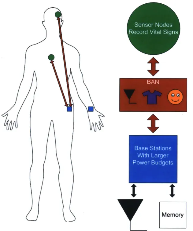
comfortably support a larger form factor enables the base station to have a larger battery. With greater power capacity, the base station can then perform the higher power functions of storing data to memory or transmitting the information off the body. Having such a base station can alleviate the power budget of the sensor node if the power required to send data to the base station is lower than the power required for the sensor node to store the data in memory or transmit it off the body. For some applications, processing can be done at the sensor node to reduce the amount of information sent over the BAN. Such a BAN can be seen in figure 1-1.

BANs have been implemented using a variety of channels, including: textiles embedded with wires [1], low power radio [2], and body coupled communication (BCC) [3]. The eTextiles have the lowest amount of signal attenuation in the channel, as the channel is simply wires, and as such the receiver doesn't need to amplify the signal and therefore energy requirements are reduced. The drawback of eTextiles is the user is required to wear specialized clothing and the sensor must be located in areas covered by the eTextiles. Forming a BAN using radio or BCC allows for greater flexibility for sensor locations, at the price of higher attenuation in the channel and hence higher power dissipation for equivalent data transmission compared to wired. BCC and ultra-wide band (UWB) radio have been shown to have similar energy per bit efficiencies, while BCC outperforms narrow band radio (NB), as seen in figure 1-2 [3].

U

Memory

Figure 1-1: Body area network diagram. There are various ways to implement body area

networks including eTextiles, radio, and BCC.

100

0p

10.

~

104

o

10.2

hm

~~A(2.

'

--

a

I

BCC

P7.3rf"

UWB

0.

10-

.

Av

NB

10

5

₁₀₆

₁₀₁

₁₀₈

₁₀

Data Rate (bps)

1.2 Use Models for BCC

There are two properties of BCC that make it highly attractive to form BANs. Both re-sult from BCC using the electric near-field which attenuates proportional to the distance cubed [4]. Because the power in the near-field signal attenuates so quickly this inherently allows for greater security than radio, because conspicuously close proximity to the body is required to connect to the network. The rapid attenuation of the signal also reduces interference from other BCC networks, which allows for reusable bandwidth.

The base station for many sensor applications could use a smartphone equipped with a BCC transceiver. As the smartphone would have to be in close proximity to the body to receive the data, the phone could be in a pocket or a case attached to the belt. If the use model for the sensor network were to render a smartphone base station impractical, a wrist watch BCC transceiver may work.

In addition to BCC replacing radio in BAN use models, like Bluetooth, BCC opens up a new use model known as "touch-to-connect". This use model utilizes the fact that devices using BCC have to be close to the body to communicate to each other; so BCC devices can assume that if two BCC nodes can talk to each other, then the nodes should automatically perform a digital hand shake and see if further communication is desired. This alleviates the step of pairing devices before they'll communicate with each other that Bluetooth requires. Touch-to-connect would allow for such use models as touching a com-puter to log-in, touching your home's door knob to unlock the door, sitting in a car seat and having your car link with your cell phone, etc.

BCC can also work with implants. This functionality means that devices such as pace-makers can use the same leads they use to regulate the heart as BCC electrodes, allowing the pacemaker to communicate with devices that are outside of the body - a much better alternative than the current method of getting signals in/out of the pacemaker's Faraday cage-like titanium can.

1.3 Contributions

There have been previous publications that have characterized the BCC channel, BCC tran-mitters, and BCC receivers [3-18]. Many of these publications have proposed channel models that disagree with each other. This work builds off these publications and devel-ops an accurate electrical channel model, validated by a custom battery-powered channel measurement system and through careful measurements. Once an accurate channel model is established, the work details two improvements to BCC communication that will aide in BCC commercialization.

This work makes three contributions to BCC technology:

1. A better understanding of the BCC channel, that is verified by careful measurements in chapter 2.

2. A new amplifier circuit has been designed and characterized, that can improve the signal to interferer ratio and detailed in chapter 3.

3. An asynchronous digital communication scheme that offers a high data rate and low power implementation. The scheme is explained in chapter 4, and an implementation of it is characterized in chapter 5.

Chapter 2

Introduction to Body Coupled

Communication

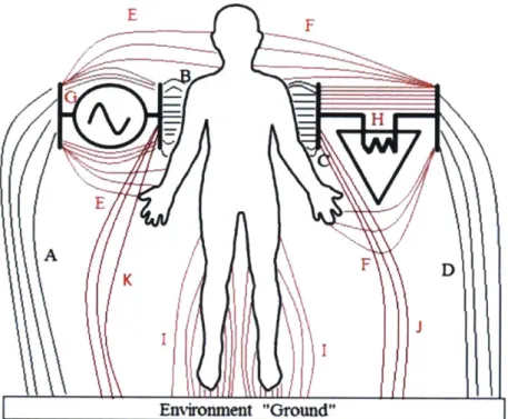
BCC makes capacitive links with the human body and the environment to form a channel in which AC current can be transmitted. Both the transmitter and the receiver have two electrodes that capacitively couple with the body and the environment. The electrodes make the capacitive links with the body and the environment by forming one plate of a parallel plate capacitor, while the other plate is formed either by the conductive tissues in the human body or the environment (figure 2-1). These capacitive links, as well as the capacitive link between the human body and the environment, form the circuit shown in figure 2-2. The environment can be anything that is conductive in the area around the human body, from a chair or table, to the physical ground itself.

E F

H

E

K F D

Emvionnmt "Groud"

Figure 2-1: The BCC channel. The electrodes on the transmitter and receiver form

capaci-tive links A-K.

K B C

G

_\(

HT

A E FD+

A

D

Figure 2-2: The circuit diagram from figure 2-1 where the color of the capacitor plates are

color coded with black to be electrodes, green the environment, and peach the body. The

resistor is the input impedance of the receiver.

Most published BCC channel models neglect to show the capacitances 'J' and 'K' be-tween the environment and the electrode as seen in figure 2-3. While it is not clear why others omit these capacitors, to keep diagrams in this work consistent with other publica-tions, this work will also omit them. This is reasonable for at least two reasons. First, the electrodes can be shielded, preventing the electrode from making such capacitive links. Second, the final BCC channel model that will be set forth in this work will show that the capacitive links 'A', 'I', 'D', 'J', and 'K' can all be ignored.

From this starting model of the BCC channel there have been opposing views on the dominant current path of the body and how the body should be modeled electrically in the

BCC channel. Some of these differences can be attributed to different frequency ranges

used in testing. As an example, the first BCC publication used frequencies in the kilo-hertz range [4], while more recent publications have used frequencies over 100 MHz. However, publications that use the same frequency range have reported different results and as such have developed different electrical models for the BCC channel. A big reason for this is the measurements methods. This work will put forth another model for the BCC channel that has been validated with multiple experiments and measured with a battery powered measurement system isolated from the environment.

I-A

C

--J

H+

LHjT4-F"

j

D

Spreading Resistance of Body

Function

Generator

0-Scope

Figure 2-4: Using equipment that shares a common node will significantly change the current paths in BCC, resulting in inaccurate measurements.

2.1

Measuring BCC Channel

Discrete battery-powered signal sources and receivers are critical to measure the BCC chan-nel. If measurement devices that are connected to an "earth ground" are used to measure the channel, such as a function generator and oscilloscope, then because these two instru-ments share the common "earth ground" between them, one electrode on the transmitter and one electrode on the receiver will be tied to the same voltage (see figure 2-4). Discrete

BCC network devices will not share such a connection with each other so what will be

measured with a transmitter and receiver that share a common reference will not remotely resemble the true BCC channel.

By shorting the nodes, current that travels through the receiver (the oscilloscope) now

has an extremely low impedance path back to the transmitter (the function generator), which will result in an inflated amount of current to run through the receiver, producing measurements that will reveal the BCC channel to have more gain than it truly does. This disparity is shown in figure 2-5, which shows the difference in the channel gain when measured with an oscilloscope and a function generator, versus with the battery-powered transmitter and receiver that will be detailed in this section. Any measurement apparatus that provides a lower impedance path from transmitter to receiver than would otherwise appear, will yield less accurate measurement results. This includes using baluns or

trans-Effects of Grounded Equipment

-20

-40

.5

-60-0

-80--e-

_{Battery Powered}

- -Grounded

Equipment

-120

-

--10

10

10

Transmitter Frequency [Hz]

Figure

2-5:

Both grounded equipment and discrete battery powered boards were used to

measure the gain in the channel. The comparison of the two measurements show

contrast-ing channel gains.

formers to isolate grounded equipment as the capacitance to the common node they provide

may be significantly greater than that which appears in the natural BCC channel.

2.1.1

Channel Measurment Equipment

To make accurate measurements of the BCC channel, a discrete transmitter and receiver

were fabricated with commercially available parts. These nodes are powered by battery

and are not connected in any way, other than through the BCC channel. The transmitter

design is shown in figure 2-6 and the receiver design is shown in figure 2-7.

The transmitter consists of an EZ430, a micro-controller radio combination that

re-ceives instructions and sets the frequency output of the AD9910 direct digital synthesizer

FTx Tx

AD-991r0

pController

+

Figure 2-6: Functional schematic of the transmitter.

Fr /$0

_dB

P

AD9910 tpController

Figure 2-7: Functional schematic of the receiver.

The outputs of this amplifier are connected to the electrodes.

The receiver consists of an amplification block made up of an ADA4817 op-amp as a

unity gain buffer (for body buffered return

-

see Chapter 3), followed by two THS4022

op-amps set for gains of 20 dB each for a total of 40 dB of initial gain. One of the receiver's

electrodes is connected to the input of the amplification block. The other electrode can be

connected to either the receiver's ground, or the output of the unity gain buffer. The output

of the amplification block is then multiplied with a signal from the receiver's AD9910 DDS.

The AD835 multiplier's output is then low-pass filtered by an LTC 1563. The filtered output

is then digitized with the ADC on the receiver's EZ430 micro-controller radio combination.

The EZ430 also sets the frequency output of the AD9910.

The receiver's DDS is set to output a sine wave that is 10 kHz higher than the frequency being measured. If the incoming signal is FT, then it will be multiplied with a sine wave with frequency FT, + 10 kHz. The output of the multiplier will be a signal with a low frequency component at 10 kHz as well as a high frequency component. After being filtered the amplitude of the 10 kHz signal will be proportional to the input amplitude of FT,. The relationship of the amplitude of the 10 kHz signal to the amplitude of FT. can be thought of as a transfer function. This relationship was measured for a range of FT. frequencies between 10 MHz- 150 MHz and will be referred to as the receiver's transfer function.

To measure the frequency response of the BCC channel the transmitter is controlled using radio to output a sine wave with a frequency of FT. The receiver is also controlled by radio to receive a sine wave of frequency FT. The 10 kHz output of the receiver is digitized and sent off the receiver, using radio, to be analyzed. Using the transfer function of the receiver, the magnitude of the 10 kHz signal can be input-referred, revealing the amplitude of the received signal at frequency FTX, which is the same as the output signal of the channel. Measuring the output voltage of the transmitter, using a high impedance probe and oscilloscope, the amplitude of the signal to the input of the channel can be captured. The channel's magnitude frequency response can then be calculated as both the amplitude of the input and output of the channel are known. Figure 2-8 shows the full test configuration.

+

Figure 2-8: The full test configuration to measure the BCC channel. The BCC channel is measured as the output of the transmiter, and input of the receiver. The channel includes all four capacitive links.

l ii

Figure 2-9: While there is a resistive element to the BCC link, the link is dominated by the

capacitance at frequencies 10 MHz and above.

2.1.2 Electrodes used for Measurements

All BCC channel measurements were made using the transmitter and receiver detailed in

section 2.1.1, unless otherwise specified. The electrodes used were the "3M 2560 Red Dot

Electrodes". By placing them on the skin a galvanic and capacitive connection is made as

modeled in Figure 2-9. The resistance through the epidermis to the conductive tissue was

found to be 1.5 MQ, while the capacitance to the conductive tissue was found to be 10 pF.

The total impedance of this connection at frequencies of 10 MHz and above is dominated

by the capacitance. Thus despite being attached to the body, these electrodes still make a

capacitive link with the body.

The resistance and capacitance values for the electrodes were found by placing multiple

electrodes on various and diverse places on a human body, such as arms, legs, torso, etc. A

multimeter was used to measure the DC resistance between each pair of these electrodes,

and an LCR meter was used to measure the capacitance between the two electrodes at

10 MHz. Regardless of the distance or position on the body of any pair of electrodes, their

capacitive and resistive values were measured to be the same.

To be clear, the purpose of this measurement was not to rigorously characterize the

electrode-body parameters. The purpose was solely to verify that using such electrodes

would produce a capacitive coupling and not a galvanic coupling. It should be stated that

2.2

Return Path

There have been conflicting publications on what the dominant current path is in the BCC channel. The dominant current path is the current loop in the BCC channel that has most of the current flowing through it. Think of the loop as a forward path and return path. The forward path of the dominant current path will be defined as leaving the transmitter, entering the body, then flowing into the receiver. The return path will be defined as the path the current takes in getting back to the transmitter from the receiver. Some publications [4, 6,8-10,14] have concluded that the dominant current path is through both the body and the environment, see Figure 2-10(a). While others [9, 12, 13, 19]concluded that the dominant current path is solely through the body as shown in Figure 2-10(b).

GD

+

B

C

G

H

I E

F114

A

LLD

Figure 2-10: Two possibilities for the dominant current path; the dominant current path is

shown with the blue loop. (a) The dominant current path as through both the body and the

environment. (b) The dominant current path as solely through the body.

Knowing the return path of the channel is important because in practice the positioning of the electrodes can be engineered to enhance the dominant current path. Note that there is no difference in the circuit models in Figure 2-10(a) and 2-10(b), just the dominant path for the current. If the return path is through the environment, then the desire is to maximize the impedance of capacitors 'E' and 'F' to force the current to flow through the environment via capacitors 'A' and 'D', as capacitors 'E' and 'F' would shunt current away from the environment. If the return path is through the body then the capacitive links 'E' and 'F' are not parasitic but are part of the desired current path and as such their impedance should be minimized.

Increasing the impedance of a capacitive link between an electrode and the body is done by increasing the distance between the electrode and the body2

, or preventing the electrode from coupling with the body by shielding the electrode. This means that if the dominant current path is through the environment one electrode, from both the transmitter and receiver, should be placed as close to the body as possible, to form capacitors 'B' and 'C', while the remaining two electrodes should be placed as far away as possible from the body to minimize the impedance of capacitors 'E' and 'F'. If the dominant current path is through the body then the best implementation would be to minimize the impedance of capacitors 'B', 'C', 'E', and 'F' by attaching both electrodes on both the receiver and transmitter as close to the body as possible [12]. Figure 2-11 depicts the differences in the ideal electrode placement for the environmental return verse the body return.

2

If a material is used as a spacer to create the distance between the body and the electrode, the mate-rial's dielectric constant should be low to further decrease the capacitive coupling between the body and the electrode.

B/C

Transmitter/

Receiver

E/F

(b)

Figure 2-11: The differences in the ideal electrode placement for the environmental return

verse the body return. (a) depicts how the transmitter's/receiver's electrodes should be

placed if the dominant current path is through the environment: one electrode as close

to the body as possible, and the other as far away as possible. While (b) depicts how

the electrodes should be placed if the dominant current path is through the body: both

electrodes are as close to the body as possible.

(a)

B/C

Transmitter/ Receiver

2.2.1

Measurments to Determine Dominant Current Path

To determine whether or not the dominant current path includes the environment return path an experiment was set up. In this experiment the channel measurement system described in section 2.1 was used. The transmitters electrodes were placed on the waist, while the receiver's electrodes were attached to the ankle of the right leg. Both electrodes on the transmitter were fixed in position on the body to keep capacitors 'A', 'B', 'E', and 'G' con-stant (refer to figures 2-1 and 2-2). One electrode on the receiver was also fixed in position on the body to keep capacitor 'C' constant. The distance to the body of the receiver's other electrode, which forms capacitor 'F', was varied using cardboard spacers. The frequency of the signal sent for the experiment was 60 MHz. The channel gain was measured as a function of the distance between the electrode and the skin, this distance being the thick-ness of the cardboard spacers. This test was run twice with about 10 minutes in between test runs. The results of these measurements, as seen in figure 2-12 are normalized such that the channel gain when the electrode is attached directly to the body has a gain of '1' or 0 dB.

However, the slope of the relationship isn't strictly decreasing, there is a point of inflec-tion where the relainflec-tionship does increase, though the increase is modest. To simulate what the electrode's capacitance would be at an infinite distance away from the body, that elec-trode was disconnected from the receiver. The channel gain was measured at this configu-ration and is the horizontal line beneath each respective curve in figure 2-12. This shows that at some distance away from the body the gain channel gain would again decrease.

10 0 -10 -20 30 -0 .cc -60' -1

Channel Gain vs Electrode Distance (Human Body)

) 0 10 20 30 40 50

Distance of Electrode From Skin [mm]

60 70 80

Figure 2-12: The channel gain as a function of the distance between an electrode and the

body; normalized when the electrode is attached directly to the body. The bottom horizontal

lines are the channel gain when the electrode was disconnected from the receiver.

--Run 1 -Run 2

-The reason for this inflection is not well understood. Perhaps there is something in

the environment that the electrode starts to couple to, as it moves away from the body,

that provides the increase in channel gain. To model this idea the circuit in figure 2-13

capacitive link of an electrode to the body, and

represents the capacitive link between

the same electrode to the environment. As the electrode moves away from the body it will

get closer to the environment. Thus the value of

decreases as the distance increases

and the value of

increases as the electrodes moves away from the body.

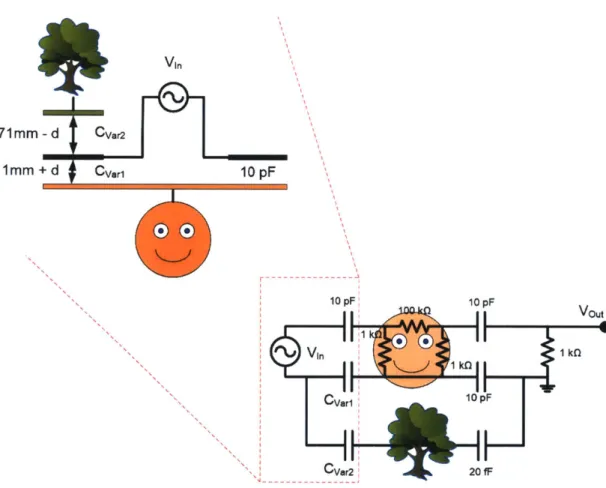
VIn 71mm - d CVar2 1mm + d Cvar1 10 pF --- ---10 pF _{10 pF} V in k Cvar1 10 pF CVar2 20 fF

Figure 2-13: A circuit model to give a possible explanation of the inflection in figure 2-12.

The voltage source, V1n, models the transmitter, the capacitors attached to the transmitter represent the capacitive links made by the electrodes and body, and one of the electrodes and environment (see figure 2-10), the three resistors (making the pi-network) model some fixed attenuation due to the body, while the resistor between Vost and ground model the input resistance of the receiver.

Mathematically the two variable capacitors were modeled as:

-

A

co

Va1 =

d+

- A₂ * 60

Var2 = 71mm _{- d}

where d is the distance in millimeters the electrode is away from the body. Cvarl was set to be 10 pF, when d was set to 0 mm, and CVar2 was set to be 2 pF when d was set to be 70 mm. The variable d was swept from 0 mm - 70 mm. The simulated gain, from

V, to Vo0 , as a function of the distance between the electrode and the body is shown

in figure 2-14 and shows an inflection in the channel gain, similar to that in figure 2-12. This simulation shows that indeed the inflection could be due to the electrode coupling to something in the environment. Note that this simulation is only meant to show that the channel gain can have a point of inflection as the electrode moves away from the body. The specific values and trends of the channel gain curve are greatly dependent on the other values of the circuit elements. The simulation is only meant to show that the inflection in the gain from figure 2-12 could be attributed to the electrode starting to couple to something in the environment more strongly as it moves away from the body.

0

-2

-4

-6

-8

10

12

Channel Gain vs Electrode Distance (Model)

0

20

40

60

Distance of Electrode from Skin [mm]

Figure 2-14: Simulated results from the circuit diagrammed in figure 2-13.

-" M

E

z--14

80

Figure 2-13 models the electrode coupling to something conductive in the environment

as the distance between the electrode and the body gets bigger. However, it could also be

that as the electrode moves away from the body fringe capacitance between the electrode

and the body develops on areas of the body that are closer to the receiver's electrodes (see

figure 2-15). The change of where fringe capacitance is coupling to on the body would

be modeled by the electrode coupling to something with a lower impedance path to the

receiver's electrodes as the distance between the body and the electrode increases. If the

impedance of the lower impedance path to the receiver's electrodes was set to zero, then

this model would reduce to that shown in figure 2-14, and thus would yield the same results

as seen in figure 2-14.

V

(a)

r$V

(b)

Figure 2-15: On the left, of both (a) and (b), is a transmitter using two electrodes to couple

to the body. A receiver is coupling to the same body with electrodes some distance away.

(a) Both of the transmitter's electrodes are close to the body. (b) By moving an electrode

farther away from the body, the fringe capacitance made by this electrode couples to areas

on the body that are closer to the receiver's electrodes.

To ensure that the inflection wasn't a source of experimental setup a similar experiment

was performed. This time instead of doing the testing on a human body, the measurement

was performed on a pork loin, and instead of cardboard spacers which can become

con-ductive when wet, plexiglass was used to control the distance. The results of the pork loin

measurement were similar to the human body measurement and are shown in figure 2-16.

Channel Gain vs Electrode Distance (Pork Loin)

-5

-10

-20

E

Z -25

-30

-10

0

10

20

30

40

50

Spacer Thickness [mm]

Figure 2-16: The channel gain as a function of the distance between an electrode and the

pork loin; normalized when the electrode is attached directly to the pork loin.

These measurements show that as the electrode was moved farther away from the

body/pork loin there was a decrease in channel gain. This means that it is better to have

all the electrodes close to the body, and that the dominant return path is through the body.

This is good for practical applications as it would be hard to shield and minimize the

ca-pacitive link of one of the electrodes with the body. This fact also will allow for implants

inside the body to communicate with devices that are outside the body, as will be shown in

section 2.4.1.

2.3 Body Model

Because the dominant current path in BCC is through the body it is important to have a model for and understand how the body's conductive tissues behave electrically. Many of the BCC papers that have thought the dominant current path is through the environment, have used electrical models for the body that aren't compatible with the dominant current path through the body. Some of the most extensive work on modeling the electrical charac-teristics of human tissue is found in [18]. Before that work will be discussed and expanded upon, the theory of how electric potentials flow through the conductive tissues of the body will be reviewed.

2.3.1

The Physical Theory

The basics of how signals can be sent through the conductive tissues of the body can be explained through a simplified example 3.

Consider an infinite medium with a uniform conductivity -. Now cut this medium in half and disregard one of the halves. The medium now spans infinity in five directions, but is bounded in the sixth direction by the cut surface. Now add hemispherical conductive electrodes E1 and E2, each with a radius 'a', into the medium such that the flat side of the

hemisphere aligns with the surface of the medium, as seen in figure 2-17. When a voltage

'V' is applied between these electrodes a current 'I' will flow. The goal is to find the

voltage, Vp, at any point in the medium due to the voltage between the electrodes. The use of super position will be used to calculate the voltage VP.

3

-

V

+

E1

E2

VP

Figure 2-17: A cross section of hemispherical electrodes placed into a medium. The

medium is infinite along five directions, and bounded by an infinite plane on the sixth.

Consider one of the hemispherical electrodes in the medium with a current 'I' being

injected into the medium from the electrode as seen in figure 2-18.

Figure 2-18: Hemispherical electrode placed into an infinite medium.

The reference electrode for both electrodes will be placed at infinity within the medium.

Having the reference at infinity will force the current to disperse uniformly

_{throughout the}

medium as shown in figure 2-19. Thus the current density at any point in the medium due

to the injected current is:

27rr2

(2.1)

where

'r'

is the distance from the center of the electrode to the point 'P' (where the current

density is being measured), E is the electric field at 'P', and a is the conductivity of the

medium.

By rearranging equation 2.1 the relationship between the electric field and the current

is:

-.

I

Ip

E =

2

r

27rr2a- 27rr2

(2.2)

The change in voltage from the electrode to point 'P', due to the current flowing from

the electrode, can be found by integrating the electric field along the path from from the

electrode to point 'P' (see figure 2-20).

4

r

Figure 2-19: The current injected into the medium will produce a uniform current density.

/ V =-j

ds=-j$dr-=

J(2.3)

AV

r

,P

Figure 2-20: The voltage difference between the electrode and the point 'P'.

This is the voltage for injecting current from an electrode into the body. To find the

voltage due to an electrode extracting current from the body, the polarity of the current

must be changed, such that:

AV'

[ -

1

(2.4)

27r

r

a

where AV' is the voltage at point 'P' due to an electrode drawing current from the body.

The solution to the goal, which is to find the voltage V at any point in the medium

-as diagrammed in figure 2-17, is simply the super position of the voltages AV and AV'.

Following from the fact that

will inject current 'I' into the medium, and E

will extract

that same current. Thus the equation for the voltage at any point in the medium is:

Ip [ 1 _(2.5)

VP = AV + AV' = - _2.I)

27L T2 r1

where r2 is the distance from E2 to the point 'P', r, is the distance from Ei to the point 'P', and V is the voltage at point 'P'.

While equation 2.5 provides the relationship between the voltage at point 'P' and the current, it is more useful to have the relationship of V as a function of the voltage between the two electrodes. To do this, we will use the boundary conditions at each electrode. It also needs to be stated that in our super position analysis from above, the voltage at Ei must be equal and opposite to the voltage at E2 to have the same current injected into the medium as the current extracted from the medium. Thus the two boundary condition equations are:

VE2 = P[i 1(2.6)

2Tr a d - a_

V~i

where d is the distance between the electrodes as seen in figure 2-17.

The voltage difference between the electrodes is V = VE2 - VEi. And thus:

Vwr

I = 7 (2.8)

P a d-a)

By plugging equation 2.8 into equation 2.5, it follows that the voltage at any point in the medium is:

VP=

[---

2( Q -a1) -r2 r1

where V is the voltage between the electrodes.

Equation 2.9 gives the relationship of the voltage at any point in the medium with respect to the the geometry/placement of two electrodes and the voltage between the elec-trodes. Now consider figure 2-21 that depicts an aerial view from above the medium's

sur-ETx1

r1

_ERx1

VP

E'Tx2

r

_ERx2

Figure 2-21: An aerial view of four Hemispherical electrodes placed on the medium's surface.

face, looking down at the surface. Two transmitting electrodes, ET,1 and ETX2, are placed on the surface of the medium. Some distance away from the transmitting electrodes, two receiving electrodes ER.i and ERx2 are placed on the same surface. If a voltage is applied between ETX1 and ETX2, then the voltage difference measured between ER.1 and ER.2 can be solved using equation 2.9. The voltage will be a scaled voltage of the input voltage between ET., and ETX2. _{The scaling factor is a function of the electrodes placement. Thus}

as long as the positions of the electrodes stay constant, then there is a linear relationship between the transmitting electrodes and the receiving electrodes, allowing signals to be sent across the medium.

This exercise has shown how a voltage generated by two electrodes in one area of the medium will produce a scaled voltage that can be measured between two electrodes in another area of the medium. This medium is analogous to the conductive tissues in the human body, with the surface of the medium being the epidermis. While the human body

is a more complex shape5, and as such will morph the boundary conditions and affect the details of how voltages will travel through the body, this basic model shows how a potential created in one area of the body, will be able to be measured at another area of the body. It is this fact, that a potential created in one area of the body -can be measured at another area, that allows BCC to work without having current flow through the environment. This exercise also shows how the position of electrodes can affect the channel gain (for more detailed experiments on the effects of electrode placement see [16]).

5

2.3.2 Spreading Resistance

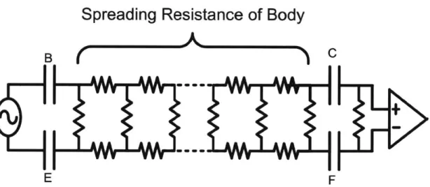
Applying finite element approach to the conductive tissues, we can imagine the tissue as a

lattice network of impedances, such as that shown in Figure 2-22. In [17] it is shown that at

frequencies between 10 kHz and 10 MHz each impedance block can be electrically

mod-eled with the circuit found in Figure 2-23 [18]. The capacitance in the impedance models

the cell membranes within the tissue, while the resistors model the resistance of the

extra-cellular and intra-extra-cellular fluid in the tissue. At some frequency the capacitive impedance

of the cell membrane will become negligible, leaving only the pure resistances to impeded

an electrical signal [19]. At that frequency and higher frequencies the conductive tissue

of the body will act as a spreading resistance. Replacing the body 'element' in Figure 2-2

with a spreading resistnace, yields the circuit in Figure 2-24.

Conductive

i

-

M.S.u

iz

Figure 2-22: The body can be modeled as a lattice work of impedances. Different types

of tissues will have different impedances and there will be transition impedances between

different tissues.

Modeling the body purely as a spreading resistance at frequencies in the range of

10 MHz -

150 MHz will be validated in section 2.4. This model also allows for the

dom-inant current path to be through the body, and is the finite element analysis model of the

physical model discussed in section 2.3.1.

Figure 2-23: The detailed model of the impedances in Figure 2-22.

B

C

G

E

X

I

41

E

T

F

A

TD

Figure 2-24: The circuit model for the BCC channel, with the body modeled as a spreading

resistance. Validated for frequencies from 10 MHz

-

150 MHz.

Re

Ztissue

Ri.

Cm