1
Applications of Risk Pooling for the Optimization of Spare Parts with
Stochastic Demand Within Large Scale Networks
By
Nigel Goh Min Feng
B.Eng. Mechanical Engineering,
The University of Western Australia, 2013
Submitted to the MIT Sloan School of Management and the MIT Department of Mechanical
Engineering in partial fulfillment of the requirements for the degrees of
Master of Science in Mechanical Engineering
and
Master of Business Administration
in conjunction with the Leaders for Global Operations Program at the
Massachusetts Institute of Technology
May 2020
© 2020 Nigel Goh, All rights reserved.
The author hereby grants to MIT permission to reproduce and to distribute publicly paper and
electronic copies of this thesis document in whole or in part in any medium now known or
hereafter created.
Author ...
MIT Sloan School of Management, Department of Mechanical Engineering May 08, 2020
Certified by ...
Nikos Trichakis, Thesis Supervisor
Associate Professor, Operations Management
Certified by ...
Kamal Youcef-Toumi. Thesis Supervisor
Professor, Mechanical Engineering
Approved by...
Maura Herson
Assistant Dean, MBA Program, MIT Sloan School of Management
Approved by...
Nicolas Hadjiconstantinou
2
3
Applications of Risk Pooling for the Optimization of Spare Parts with
Stochastic Demand Within Large Scale Networks
By
Nigel Goh Min Feng
Submitted to MIT Sloan School of Management and the MIT Department of Mechanical
Engineering on May 08, 2020 in partial fulfillment of the requirements for the degrees of Master
of Business Administration and Master of Science in Mechanical Engineering
Abstract
Amazon is able to deliver millions of packages to customers every day through its Fulfillment Center (FC) network that is powered by miles of material handling equipment (MHE) such as conveyor belts. Unfortunately, this reliance on MHE means that failures could cripple an entire FC. The exceptionally high stock-out cost associated with equipment failure means spare parts must always available when required. This is made difficult as Amazon does not hold any central repository of inventory at present – all inventory is held at a site-level. Unfortunately, FCs have to stock more inventory than required due to unpredictable failures, long lead times from suppliers, and no standard work processes for site-to-site transfers. However, if Amazon is able to pool its spares across multiple FCs, it has an opportunity to reduce the spares kept across the entire FC network, position itself to better respond to catastrophic failures, and consolidate interfaces with suppliers.
The goal of this thesis is to identify the inventory model and network design that would maximize parts availability while minimizing cost. Additionally, an implementation roadmap will be developed to outline how such a system (e.g. hub locations, logistic channels etc.) can be developed. This thesis concludes by proposing potential extensions of the work conducted in this thesis to improve the practicality and financial impact of the proposed network and inventory model.
Thesis Supervisor: Kamal Youcef-Toumi Title: Professor of Mechanical Engineering, MIT
Thesis Supervisor: Nikos Trichakis
4
The author wishes to acknowledge the
5
Acknowledgements
I would like to first thank my MIT academic advisors, Professors Nikos Trichakis and Kamal Youcef-Toumi, who both took significant amounts of time out of their busy schedule to provide guidance and direction throughout my internship. This thesis would not be anything close to what it is if not for their help, and I am tremendously privileged to have had the opportunity to learn from them.
I would also like to thank Amazon for the opportunity to work on what is an essential part of their operations, and for the support that they have provided through the entire process. I want to also specifically thank John Fogerty, who was both manager and friend, for his trust and constant feedback. Additionally, I’d like to thank Brent Yoder who championed my project from start to finish, and was instrumental in ensuring that the project stayed on track and never ran into problems.
Next, I can’t possibly write acknowledgements without writing about my LGO classmates – an amazing group of people who keep me grounded and humble every day. I am extremely thankful for their friendship and for making these two years at MIT a remarkable experience that I will always remember.
Finally, I would like to thank my family. I’m only where I am today because of their love, encouragement and support. Thank you for helping me (try to) be the best person that I can be. I am, and will be, forever grateful to them for everything they have done for me.
6
Table of Contents
Abstract ... 3 Acknowledgements ... 5 Table of Contents ... 6 List of Figures ... 9 List of Tables ... 9 1. Introduction ... 10 1.1. Project Background ... 10 1.2. Problem Statement ... 101.3. Research Hypothesis and Methodology ... 11
1.4. Project Scope and Limitations... 12
2. Literature Review ... 14
2.1. Inventory Theory ... 14
2.2. Inventory Models ... 16
2.2.1. Newsvendor and Economic Order Quantity ... 16
2.2.2. (R,Q) Inventory Model ... 17 2.2.3. (S-1, S) Inventory Model ... 18 2.3. Inventory Pooling ... 19 3. Methodology ... 21 3.1. Research Hypothesis ... 21 3.2. Data Analysis ... 22 3.3. Model Development ... 23 3.4. Summary ... 26
4. Data Breakdown and Analysis ... 27
4.1. Current State ... 27
7
4.2. Estimating Missing Data ... 29
4.3. Improving Data Accuracy – Returns and Outliers ... 34
4.4. Data Analysis ... 37
4.4.1. Aggregation of Data ... 37
4.4.2. Managing Peak Seasons ... 38
4.5. Summary ... 39
5. Inventory Model Development ... 40
5.1. Newsvendor Model ... 40
5.1.1. Potential Distribution Types ... 42
5.1.2. Distribution Selection ... 46 5.2. EOQ ... 47 5.2.1. EOQ Optimizations ... 48 5.3. (R, Q) Inventory Policy ... 53 5.4. Conclusion ... 54 6. Multi-Echelon Inventory ... 56 6.1. Multi-Echelon Systems ... 56
6.2. Facility Location Analysis ... 57
6.2.1. Potential Hub Locations ... 58
6.2.2. Distance Calculations ... 59
6.2.3. Zone Modelling ... 60
6.3. (S-1, S) vs (R, Q) Inventory Models in Multi-Echelon Networks ... 61
6.4. Hub Selection ... 62
6.4.1. Inventory Placement ... 63
6.4.2. Shipping Costs ... 68
6.4.3. Frequency of Delivery ... 71
8
6.6. Sensitivity Analysis ... 76
6.6.1. Lead Time Reduction ... 76
6.6.2. Cost Reductions ... 77
6.6.3. Criticality Service Levels ... 78
6.7. Operations Within a Nodal System ... 79
6.8. Risks and Challenges ... 80
6.9. Summary ... 80
7. Conclusion and Recommendations ... 81
7.1. Summary of Findings ... 81
7.2. Next Steps ... 82
7.3. Future Work ... 83
9
List of Figures
Figure 2.1: (a) Deterministic vs (b) Stochastic Demand ... 15
Figure 4.1: Example of part consumption in various sites in 1st week of 2014 ... 28
Figure 4.2: Lead Time Distribution for Parts ... 31
Figure 4.3: Sample Week-By-Week Demand for 3 Parts ... 34
Figure 4.4: Example of Negative Usage Data for Part 10022 in Site ABE2 ... 34
Figure 4.5: Consumption of Parts by Cost (Original vs Smoothed) ... 35
Figure 4.6: Consumption of Parts by Cost (Before / After Adjustment) ... 36
Figure 4.7:Weekly Consumption Parts (by Number of Parts) ... 36
Figure 4.8: Price vs Total Cost / # of Parts ... 37
Figure 4.9: Scale Adjusted Consumption Plots ... 38
Figure 5.1:Newsvendor Diagram ... 41
Figure 5.2: Increase in Shipping Costs due to EOQ Constraint ... 49
Figure 5.3:EOQ Constraints: Shipping Costs vs NPV Savings ... 51
Figure 5.4:EOQ Constraints: Overall Cost Savings ... 51
Figure 5.5: EOQ Constraints (Overall Savings) ... 52
Figure 6.1: Selection of Potential Hub Locations ... 59
Figure 6.2: Current Structure vs Multi-Echelon Network ... 63
Figure 6.3: Shipping Costs vs. Shipping Frequency (days) ... 72
Figure 6.4:Cost vs Total # of Zones (Various Hub Configurations) ... 74
List of Tables
Table 1.1: Current Stocking of SKUs ... 11Table 4.1: Parameters from SQL ... 29
Table 4.2: Median vs Mean Price ... 32
Table 5.1: Criticality to Service Level Mapping ... 42
Table 5.2: Mean vs Variance Distribution of Dataset ... 44
Table 5.3: Best-Fit Distribution Types ... 46
Table 5.4: Performance of Distributions vs Best-Fit ... 47
Table 5.5: EOQ Constraints ... 49
Table 5.6: EOQ Constraints: Shipping Costs vs NPV Savings ... 50
Table 5.7: Criticality to Service Level ... 53
Table 5.8: Differences in Inventory Levels (Current Min/Max vs Proposed (R,Q) Model) ... 54
Table 6.1: Example of Third-Party Shipping Rates ... 60
Table 6.2: Shipping Zone Multipliers ... 61
Table 6.3: Example of Inventory Policies for One Part ... 65
Table 6.4: (R,Q) vs (S, S-1) Breakdown for Multi-Echelon System (No Shipping) ... 68
Table 6.5: Total Incremental Shipping Costs (Perpetuity) ... 69
Table 6.6:Shipping Costs with Updated Pricing Model... 70
Table 6.7: Inventory Value and Shipping Costs ... 70
Table 6.8: Shipping Frequency to Shipping Costs ... 72
Table 6.9: Total Cost vs Shipping Frequency ... 73
Table 6.10: Cost Ranges for 30 Potential Hub Locations ... 75
Table 6.11: Cost Comparison of Inventory Policies ... 75
Table 6.12: Sensitivity Analysis: Supplier Lead Time ... 76
Table 6.13: Hub to FC Lead Times... 77
Table 6.14: Sensitivity Analysis - Hub to FC Lead Time ... 77
Table 6.15: Sensitivity Analysis - Delivery Costs ... 78
Table 6.16: Sensitivity Analysis - Price Reduction ... 78
10
1. Introduction
1.1. Project Background
Amazon is able to fulfill its two-day delivery promise and deliver millions of packages to its customers every day through its Fulfillment Center (FC) network, where FCs hold inventory that is available for sale on Amazon. When a customer places an order online, the order is assigned to an FC that has the item in stock, and the item is then packed and shipped to the customer. The FC network is powered by miles of material handling equipment (MHE), such as conveyor belts and rollers, that help to move the inventory across the FC.
In order to ensure that customers are able to receive their packages on time, FCs are required to hold spare parts for all MHE. This ensures that any breakdowns can be immediately repaired and will not disrupt any flow of inventory within, and out of, the FCs.
1.2. Problem Statement
Amazon’s ability to deliver on its two-day promise to customers is highly reliant on the continuous operation of Material Handling Equipment (MHE) within the various Fulfilment Centers (FCs). This dependence on MHE means that equipment stock-outs could have significant consequences for operations. As such, Reliability and Maintenance Engineering (RME) must ensure MHE spares are always available when required. However, holding an excessive amount of MHE parts is neither feasible nor desirable due to space and cash flow constraints.
Inventory levels are currently controlled through a Min/Max inventory policy. However, the Min/Max levels are set based on vendor recommendation and site admin experience, not usage data of the parts. Variability in demand for parts and long lead times (typically four weeks or more) make it difficult to accurately determine optimal stocking volumes for MHE spares. Comparisons against a data-based
11
inventory model show that only 30.2% of current parts are stocked at an optimal level. This means that many NAFC sites are either holding excess inventory or not holding enough inventory (increasing the risk of a stock-out).
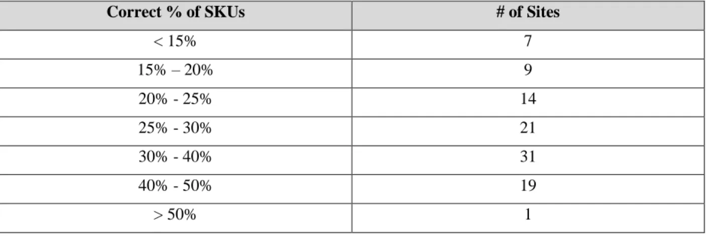
The table below show how 102 NAFC sites (with >500 parts in stock) perform in terms of having a certain proportion of their SKUs within percentage bands of “optimal” stocking values based on best practice inventory policies. This data is not included as a precursor for further analysis on current stocking policies, but rather seeks to simply shed light on the potential of this program.
Correct % of SKUs # of Sites
< 15% 7 15% – 20% 9 20% - 25% 14 25% - 30% 21 30% - 40% 31 40% - 50% 19 > 50% 1
Table 1.1: Current Stocking of SKUs
This is further complicated as Amazon does not have a central repository for inventory, so parts are ordered directly from suppliers. Each FC manages its own budget and inventory through an Enterprise Asset Management (EAM) software and a dedicated site-based EAM administrator who is responsible for the spares cage in the FC. Since FCs are managed at the site-level, and not as a network, it is difficult to identify duplicate parts between sites, consolidate suppliers (and leverage Amazon’s buying power), and better respond to emergencies and stock-outs by sharing parts between sites in the network.
1.3. Research Hypothesis and Methodology
This presents two opportunities to improve FC operations across the entire network. First, Amazon has significant amounts of data regarding spare parts usage that could be used to better inform stocking levels
12
of spare parts. Second, risk-pooling between sites can be implemented to share and manage parts at the network level.
Risk-pooling creates a multi-echelon supply chain by introducing centralized hubs within the FC network that FCs can source parts from. This significantly lowers part lead times at an FC-level and also pools the demand for spares across multiple FCs – both of which help to reduce inventory levels. This “nodal warehousing” strategy presents an opportunity for Amazon to not only reduce the spares kept across the FC network, but to also position itself to better respond to catastrophic failures whilst consolidating interfaces both internally (e.g. inventory planners) and externally (e.g. vendors).
As such, there were two key goals for this project. First, to identify the optimal risk-pooling design for Amazon’s FCs and to quantify any potential savings that would result from its implementation. Second, to use data to determine the optimal part stocking levels that would maximize part availability while minimizing cost.
1.4. Project Scope and Limitations
Due to the scale of Amazon’s operations, in order to ensure that the project could be done within the available timeframe, only Amazon’s North American operations were considered. Although the scope of work from this project could be extended to other geographies, there are other factors that will have to be considered when doing so (e.g. cross-border complexities between countries).
A core part of this project involves the use of data regarding spare part usage and ordering. One limitation of this data is that it is extracted from a system that involves manual input from users, and there are observations where those manual inputs are incorrect. However, due to the number of data entries within the system, it is not feasible for the data to be manually filtered. As such, systems will be put in place to identify and filter out incorrect data entries where possible, but all other data entries will be taken as accurate.
13
This study also assumes that inventory levels cannot be run down to zero (i.e. where FCs use a pull system when spares are required) as that would necessitate downtime whenever a spare is required. As the priority for FCs is to ensure that there is no downtime, this is considered to be not acceptable.
Finally, although Amazon made all its data available as part of this thesis, for data privacy reasons, all data that is specific to Amazon was presented to Amazon at the conclusion of the project and will not be reproduced within this thesis. Instead, this paper will focus on the process and general learnings that are applicable to other scenarios.
14
2. Literature Review
Spares management and inventory modelling are well-established areas of operations research. This chapter aims to provide an overview of the prior work already done in this space and to establish the context required to understand the other chapters of this paper. The literature review then also looks into potential ways in which risk-pooling can be applied to supply chains, and provides a glimpse into the facility location problem – the problem of placing warehouses in an optimal location.
2.1. Inventory Theory
One key challenge for any operation involving variable demand (e.g. retailers, warehouses etc.) is determining the quantity of inventory to hold. If the operation does not hold sufficient inventory, they risk running out of stock which could result in lost sales or downtime. On the other hand, excess inventory ties up cash flow and space, both of which could be used to improve the operation in other ways, and typically has associated holding costs.
Another inventory management challenge lies in restocking of inventory. Inventory typically has to be ordered in advance of when they are required due to lead times from suppliers (which typically adds another dimension of variability). This is further complicated as inventory will be further consumed while waiting for new inventory to be delivered from suppliers. As such, inventory managers have to determine how much inventory to order, and when to order that inventory before they have sufficient data to do so. Due to the highly visible consequences of stockouts, there is a temptation for warehouses/retailers to hold more inventory than required.
In response to these challenges, mathematical inventory models have been developed to improve inventory policies which provide guidance on timing and quantities of inventory replenishment. Although there are many different models, there are several distinctions that are of particular interest to this paper:
15
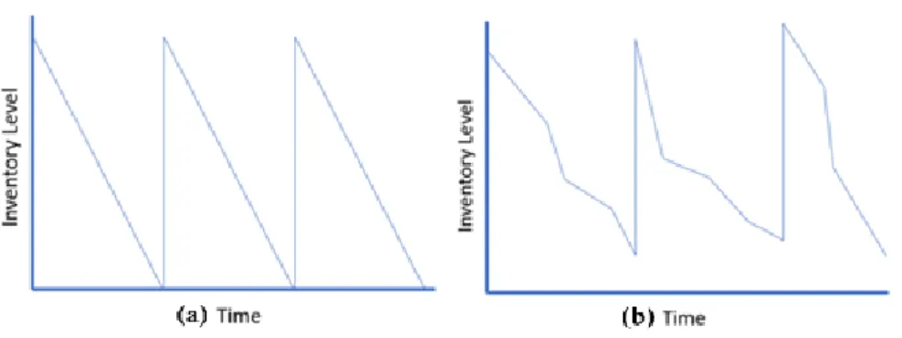
1) Deterministic vs Stochastic Demand: Demand profiles will vary depending on the type of function the inventory is used for. If future demand is well-known and can be accurately forecasted, a deterministic inventory model is used. However, if future demand is a variable rather than a known constant, then a stochastic inventory model has to be used (Jensen & Bard, 2002).
Deterministic demand profiles consume inventory continuously at a known and constant rate, whereas stochastic demand profiles have uncertainty in the demand. In both cases, inventory is replenished when needed by ordering a certain replenishment quantity. (b)
Figure 2.1: (a) Deterministic vs (b) Stochastic Demand
2) Single vs Multi Period: An inventory model has to determine the correct amount of inventory to stock in order to optimize costs and/or profits. However, the model may be used for a single period (i.e. once the period is over, the parts are no longer required), or for multiple periods. A single period considers inventory as independent of future periods, whereas multi-period models carry over inventory from period to period, which complicates the inventory policy (Zhang et al., 2009).
3) Periodic vs Continuous Review: For multi-period inventory models, any consumed inventory will typically have to be replenished at some point in time. A periodic review model checks the inventory level at specific intervals, and replenishment orders are only made during those time windows. In a continuous review model, inventory is continuously monitored, and an order is
16
placed as soon as the inventory level falls below a certain threshold known as the reorder point (Zappone, 2006).
For the purposes of this paper, Amazon faces a stochastic demand over multiple periods, but is able to implement a continuous review process.
2.2. Inventory Models
2.2.1.
Newsvendor and Economic Order Quantity
Any operation with fluctuating demands will typically face issues as the demand uncertainty could result in overstocking and stockouts. Numerous inventory models have been developed over the years to deal with this and the newsvendor model has been a mainstay of inventory theory since it was developed in 1951 by Morse and Kimball.
The newsvendor model applies to scenarios where an operation faces stochastic demand and has to determine its required quantity of inventory before knowing the required demand (Morse & Kimball, 1951). The overall objective of the newsvendor model is to identify the inventory quantity that best balances the overage and underage costs through statistical information on the demand (e.g. the mean and standard deviation of the demand). Using the newsvendor model, it is possible to determine a level of carrying inventory that is required to meet the expected demand for a given period of time.
The newsvendor model typically assumes a normal distribution due to its ease of application. However, due to a high probability of negative demands (which is not theoretically possible) when the mean is low and variability is high, the normal distribution may not be a reasonable approximation of the demand all the time. As such, in the event of a high coefficient of variation of demand, typically defined as >0.5, one should consider a distribution other than a normal distribution (Halkos & Kevork, 2012; Silver et al., 1998).
17
Although the newsvendor model is able to provide operations with a sense of how much inventory is required for a single period, it does not help to determine how much inventory to reorder to make up for consumed parts. The Economic Order Quantity (EOQ) was first developed by Ford Whitman Harris in 1913 and can be applied to inventory items that are replenished in batches. The EOQ model considers two cost buckets, holding costs and ordering costs, and aims to minimize the combined cost of both (Goh, 1994).
2.2.2.
(R,Q) Inventory Model
Although the newsvendor model and EOQ provide a baseline upon which an inventory policy can be built, there are more specialized inventory models that are more applicable to Amazon. The (R,Q) inventory model typically involves a continuous review period over multiple periods, and is better suited for Amazon’s purposes.
The (R,Q) policy assigns a fixed replenishment point and a fixed replenishment quantity for each part. The (R,Q) model has two parameters: whenever the inventory on hand falls below a certain Reorder Point (R), it will trigger a new order for a specific Reorder Quantity (Q). The reorder point is set such that there is sufficient inventory on hand to meet all reasonably expected demands while waiting for the replenishment quantity from the supplier. Reorder quantities are set to minimize the total cost of ordering and holding inventory through the EOQ (Cachon & Terwiesch, 2013; Capar & Eksioglu, 2009).
Reorder Level (R)
The Reorder Level is the inventory quantity at which new inventory is ordered. Intuitively, when a new order is placed, the system must ensure that there are sufficient parts on hand to cover demand until the new parts arrive. Accordingly, this Reorder Level for any part corresponds to the sum of the Cycle Stock and the Safety Stock. These terms are described further below:
18
1) Cycle Stock is the inventory that is expected to be used for any given period of time. This time interval is typically the lead time for the part (i.e. How many parts will be used while waiting for new parts to arrive).
𝐶𝑦𝑐𝑙𝑒 𝑆𝑡𝑜𝑐𝑘 [𝑃𝑎𝑟𝑡𝑠] = 𝐴𝑣𝑒𝑟𝑎𝑔𝑒 𝐷𝑒𝑚𝑎𝑛𝑑 𝑝𝑒𝑟 𝑇𝑖𝑚𝑒 (𝜇) [𝑃𝑎𝑟𝑡𝑠
𝑇𝑖𝑚𝑒] ∗ 𝐿𝑒𝑎𝑑 𝑇𝑖𝑚𝑒 [𝑇𝑖𝑚𝑒]
2) Safety Stock refers to the additional inventory that is kept on hand to account for weeks that have larger than expected demand requirements (as it is impossible to predict the exact amount used every week).
𝑆𝑎𝑓𝑒𝑡𝑦 𝑆𝑡𝑜𝑐𝑘 [𝑃𝑎𝑟𝑡𝑠] = 𝑆𝑡𝑎𝑛𝑑𝑎𝑟𝑑 𝐷𝑒𝑣𝑖𝑎𝑡𝑖𝑜𝑛 (𝜎) [𝑃𝑎𝑟𝑡𝑠
𝑇𝑖𝑚𝑒] ∗ √𝐿𝑒𝑎𝑑 𝑇𝑖𝑚𝑒 [𝑇𝑖𝑚𝑒] ∗ 𝑆𝑎𝑓𝑒𝑡𝑦 𝐹𝑎𝑐𝑡𝑜𝑟 The Safety Factor is the z-score corresponding to a part’s desired service level on the normal distribution (i.e. a Safety Factor of 3 will ensure sufficient inventory to cover inventory requirements 99.7% of the time -- a 99.7% service level).
Reorder Quantity
As more parts are ordered, the “cost per part” decreases due to fixed costs being spread across more parts. However, this is countered by the increased cost of holding more inventory. The Reorder Quantity (Q) aims to minimize the total cost of placing an order by optimizing for both ordering costs and holding costs.
𝑄 [𝑃𝑎𝑟𝑡𝑠] = √2 ∗ 𝐷𝑒𝑚𝑎𝑛𝑑 [ 𝑃𝑎𝑟𝑡𝑠
𝑇𝑖𝑚𝑒 ] ∗ 𝐹𝑖𝑥𝑒𝑑 𝑂𝑟𝑑𝑒𝑟𝑖𝑛𝑔 𝐶𝑜𝑠𝑡 [$] 𝐻𝑜𝑙𝑑𝑖𝑛𝑔 𝐶𝑜𝑠𝑡 [𝑇𝑖𝑚𝑒 ∗ 𝑃𝑎𝑟𝑡] $
Whilst most parameters are fixed, the holding cost may be set based on numerous factors. Berling presents a general model based on microeconomics through which a holding cost can be determined (Berling, 2008).
2.2.3.
(S-1, S) Inventory Model
An alternate model to the (R,Q) inventory model is the base stock model, also known as the (S-1, S) model. The (S-1, S) model works like the (R,Q) model in most ways. The main difference lies in how parts are
19
replenished. The (S-1, S) model sets the required inventory level at (S), and whenever parts are consumed, it immediately replenishes its inventory back to the required inventory level of “S” (Cachon & Terwiesch, 2013). This is also known as an “order up to” inventory model, as it will replace any consumed inventory up to the required threshold.
The (S-1, S) model can also be thought of as an (R,Q) model with a reorder level of (S-1) and a reorder quantity of 1.
2.3. Inventory Pooling
Inventory pooling is a well established branch of operations research that was first introduced by Eppen in 1979 (Eppen, 1979). The concept of inventory pooling has been further explored since 1979, and it has been shown that pooling works across different demand distribution types (Federgruen & Zipkin, 1984). At a high level, inventory pooling combines various demand streams together in order to minimize the effects of demand uncertainty as the pooled demand will help to balance high and low demand variations (Bimpikis & Markakis, n.d.).
Graves and DeBodt show that it is possible to extend the traditional (R,Q) inventory model to a multi-echelon supply chain with reasonable accuracy (DeBodt & Graves, 1983). Additionally, Axsäter shows that, for multi-echelon supply chains with low demand, it is suitable to apply continuous review policies as opposed to needing to use a periodic review policy for high demand items (Axsäter, 1993).
Multi-echelon systems do not reduce the average demand of its constituent FCs. If the system needed 10 parts per week, it will still use 10 parts per week after nodal warehousing is introduced. As such, weekly consumption of Cycle Stock, which is defined through demand levels, are not affected by pooling.
The benefit of pooling comes from reductions in demand variability which reduces Safety Stock levels. Safety stocks at an FC-level drop due to a lead-time reduction. At a systems level, safety stock reductions
20
occur by combining variations. Assume that there are three sites, each with a part with a standard deviation of 5. Using the formula above, the “combined” standard deviation is 8.66 (as opposed to the total standard deviation of 15 if they were kept separate). This almost halves the amount of safety stock that need to be held within the network to cover for demand fluctuations.
21
3. Methodology
This chapter details the research expectations of this project, the steps required for the data analysis and inventory model development, the risk-pooling methodologies, and the various considerations that went into improving and selecting the final model.
3.1. Research Hypothesis
As failures can occur at any time, there is much uncertainty surrounding the rate of spare part consumption. This is one of the major factors that complicates spare parts stocking levels at Amazon FCs. Given Amazon’s desire for 100% uptime on MHE, FCs must ensure they have sufficient spare parts on-hand at any given time. Unsurprisingly, this could result in many FCs holding more parts than required. This study expects that inventory levels across the FC network can be optimized in two ways.
First, historical data on parts consumption can be used to advise stocking quantities. The EAM system has access to part data (e.g. price, lead times etc.) and demand profiles for each part over the last five years. The demand profiles can be used to determine an expected mean and standard deviation for the consumption of each part over a given period of time. These parameters can be used alongside the available part data to determine an optimal stocking quantity for each part through an inventory model, such as the (R,Q) model described in Chapter 2.
The second way is through risk-pooling across sites through a multi-echelon supply chain to minimize demand variations across the network. At present, all FCs individually manage their inventories with minimal sharing between sites. This exposes every FC to high variability in week-to-week part consumption. These demand fluctuations result in sites needing to stock enough parts to deal with weeks of high part consumption, even when those weeks of high demand do not happen often. A central warehouse for risk-pooling will normalize weekly demand across the entire network, and should result in lower carrying volumes of spare parts.
22
The central warehouse should stock all the required spared, and FCs can order parts directly from the central hub. This will dramatically shorten lead times for FCs to a matter of days. As shown by the equation for the reorder point, a shorter lead time will lower the quantity of parts that each site has to hold.
𝐶𝑦𝑐𝑙𝑒 𝑆𝑡𝑜𝑐𝑘 [𝑃𝑎𝑟𝑡𝑠] = 𝐴𝑣𝑒𝑟𝑎𝑔𝑒 𝐷𝑒𝑚𝑎𝑛𝑑 𝑝𝑒𝑟 𝑇𝑖𝑚𝑒 (𝜇) [𝑃𝑎𝑟𝑡𝑠
𝑇𝑖𝑚𝑒] ∗ 𝐿𝑒𝑎𝑑 𝑇𝑖𝑚𝑒 [𝑇𝑖𝑚𝑒]
𝑆𝑎𝑓𝑒𝑡𝑦 𝑆𝑡𝑜𝑐𝑘 [𝑃𝑎𝑟𝑡𝑠] = 𝑆𝑡𝑎𝑛𝑑𝑎𝑟𝑑 𝐷𝑒𝑣𝑖𝑎𝑡𝑖𝑜𝑛 (𝜎) [𝑃𝑎𝑟𝑡𝑠
√𝑇𝑖𝑚𝑒] ∗ √𝐿𝑒𝑎𝑑 𝑇𝑖𝑚𝑒 [𝑇𝑖𝑚𝑒] ∗ 𝑆𝑎𝑓𝑒𝑡𝑦 𝐹𝑎𝑐𝑡𝑜𝑟 The network as a whole does not benefit from the shorter lead time (as the central hub still has to order from suppliers with the same four to six week lead time), but benefits from pooled demand as combined variance/standard deviation is lower than the sum of its parts as shown below:
𝜎𝑝𝑜𝑜𝑙𝑒𝑑= √∑(𝜎12+ 𝜎22… + 𝜎𝑛2) 𝑛
𝑖=1
Intuitively, this can be understood as a higher week of consumption in one site will, when spread over hundreds of sites, be balanced out by a week of lower consumption in a different site. This will lower the required safety stock that needs to be held across the network. Note that the cycle stock (i.e. the amount that is expected to be consumed every week) is not affected by this change. There is also a possibility that centralized stocking and ordering will provide Amazon will more market power to negotiate shorter lead times with suppliers, but we assume its effect to be zero for the purposes of this study.
3.2. Data Analysis
The EAM data forms the foundation upon which the rest of the project is built. Although a large amount of information is available on Amazon’s servers, not all the information is relevant. Accordingly, any
23
necessary data must first be identified, before then extracting the data from Amazon’s servers through SQL queries. The accuracy/completeness of these queries must then be validated to ensure that
As much of the data on EAM was filled in manually, there is a non-zero possibility of inaccuracies in the data. The data thus has to be filtered to determine what can be used, and what has to be excluded from the study. Due to the size of the data sets used, it was not possible to validate the data at an individual level. Issues were identified by trending and aggregating data, which highlighted areas that needed further investigation. For example, parts that were returned late resulted in choppy data that skewed weekly consumption numbers.
These data trends provided valuable insights into not only data inaccuracies, but also key areas for improvement. For example, there were specific part types that accounted for a large proportion of weekly demand, and warranted special attention and focus. However, for data privacy reasons, the results from this section are not explored as part of this thesis as they do not provide any general learnings. Instead, they formed part of the internal recommendations that were made available Amazon through this thesis.
Finally, in order to maximize the applications for this study, data that was missing from EAM was estimated where possible. Only parameters that could be ascertained with a high degree of confidence (e.g. FCs may not have a price assigned to a part, but the part’s price is known across the network) was included in the study.
3.3. Model Development
Once all of the data is verified and made available, it is possible to then fit the parameters for every part into an inventory model. The (R,Q) model was chosen to establish a specific inventory policy for every part in FCs due to its ease of use and continuous review period. First, the study considers how an application of the (R,Q) inventory model will affect inventory levels without the use of risk-pooling. This will enable effective evaluation of the impacts of applying an inventory policy by comparing the new inventory
24
numbers to the current state. Additionally, this will also establish a baseline to evaluate the impacts of risk-pooling and whether it is worth pursuing. For example, if risk-risk-pooling only reduces inventory levels by 2%, it may not be worth the capital and effort required to set up the multi-echelon model.
Once the baseline (R,Q) model is established, it is possible to explore other inventory models and perform sensitivity analyses to identify key parameters that affect the overall inventory policy and where the biggest rooms for improvements are. Again, for data privacy reasons, the results from this section are not included in this paper as they do not provide any general learnings.
The final step involves the inclusion of risk-pooling into the overall network through a multi-echelon system (also called nodal warehousing system in this thesis) that lowers inventory levels in the system by pooling variability. The key outcomes desired from this phase of the project was a determination of the number of nodal warehouses to be used, as well as the locations of those warehouses.
A singular nodal warehouse will “pool” the most parts together, and should result in a lower inventory level. However, these gains could be undermined by longer lead times to FCs (a singular warehouse would increase the net distance between hubs and FCs) and/or higher shipping costs. For the purposes of this study, it is assumed that the shipping cost from suppliers to the hub is equivalent to existing shipping costs. As such, any incremental shipping cost will be the result of the extra shipping leg between the hub(s) and the FCs.
First, potential hub locations have to be identified, and the distance between those hub locations and FCs have to be mapped (to accurately predict shipping costs and lead times). Next, the demand parameters for each FC/hub need to be determined. In multi-echelon inventory, each FC is considered a separate entity. Fortunately, the (R,Q) model also applies to multi-echelon systems. The only difference is that the hub’s inventory is not simply the physical inventory on-site, but also includes all inventory downstream of it. This formula is applied to each part to ascertain the overall network inventory level for every part:
25
For example, if a hub has one motor on its shelves, and it supports two sites, each holding one motor, the inventory level of the hub is three motors. It is this combined inventory that triggers the Reorder Point.
The lead time for the hub, for the purposes of (R,Q) model implementation, is given by the maximum amount of time it takes to get from a supplier to an FC (through the hub):
𝐻𝑢𝑏 𝐿𝑒𝑎𝑑 𝑇𝑖𝑚𝑒 = 𝑇𝑖𝑚𝑒 𝑓𝑟𝑜𝑚 𝑆𝑢𝑝𝑝𝑙𝑖𝑒𝑟 𝑡𝑜 𝐻𝑢𝑏 + max (𝐿𝑒𝑎𝑑 𝑇𝑖𝑚𝑒ℎ𝑢𝑏−𝑡𝑜−𝐹𝐶)
Essentially, the hub and its FCs are treated as one “giant site” with the combined demands of all its constituent FCs. For example, assume a hub supports two FCs, each requiring one part a week. Assume also that it takes four weeks for a part to get from supplier to the hub, and it takes one week to go from the Hub to the FCs. This is the same as one giant site that uses two parts a week, with a lead time of five weeks. Demand profiles are treated in a similar way, except the hub has no demand of its own. Pooled demand parameters are calculated as follows:
𝐴𝑣𝑒𝑟𝑎𝑔𝑒 𝑆𝑦𝑠𝑡𝑒𝑚 𝐷𝑒𝑚𝑎𝑛𝑑 = ∑ 𝐴𝑣𝑒𝑟𝑎𝑔𝑒 𝐷𝑒𝑚𝑎𝑛𝑑 𝑜𝑓 𝑃𝑎𝑟𝑡 𝑎𝑡 𝐹𝐶𝑛 𝐴𝑙𝑙 𝐹𝐶𝑠 𝑛=1 𝑆𝑦𝑠𝑡𝑒𝑚 𝑆𝑡𝑎𝑛𝑑𝑎𝑟𝑑 𝐷𝑒𝑣𝑖𝑎𝑡𝑖𝑜𝑛 = √ ∑ (𝑆𝑡𝑎𝑛𝑑𝑎𝑟𝑑 𝐷𝑒𝑣𝑖𝑎𝑡𝑖𝑜𝑛 𝑜𝑓 𝑃𝑎𝑟𝑡 𝑎𝑡 𝐹𝐶𝑛)2 𝐴𝑙𝑙 𝐹𝐶𝑠 𝑛=1
These parameters allow for the (R,Q) model to be applied to every possible hub configuration (both location and quantity) to identify the best configuration. As nodal warehousing will increase shipping costs (due to additional shipping between the central warehouse and the FCs) but reduce inventory volumes, the optimal solution would be defined by the most significant reduction in overall cost.
26
3.4. Summary
Inventory models can provide guidance on inventory stocking policies at an individual FC level. In the particular case of Amazon, the (R,Q) model was chosen due to its continuous review period and easy applicability. After the (R,Q) model is applied to each FC, the entire network can be further optimized through risk-pooling, which can further reduce inventory levels by reducing overall demand variability across different sites.
27
4. Data Breakdown and Analysis
As shown in Chapter 3, a large amount of data is required to apply the required models. This chapter details how that data was managed as part of this thesis. It explores the available data from EAM, how missing parameters were estimated based on available information, and how data accuracy was improved through systemic elimination of outliers. It then looks at how the final dataset can be aggregated and used to draw further conclusions regarding the overall state of the supply chain.
4.1. Current State
The bulk of the data used for this project was extracted from Amazon’s Enterprise Asset Management (EAM) software which captures most of the information regarding Amazon’s spare parts. However, the data on EAM is not populated automatically, and instead relies on EAM admins to manually input most parameters (e.g. price of part, quantity purchased/consumed etc.) In the past, EAM served as a platform for tracking data, but this data was not always utilized. As such, there was no incentive for EAM admins to ensure 100% data accuracy on EAM. This has resulted in some parts not having all the data required for further analysis (e.g. price, lead time, usage data etc.) and other parts having inaccuracies within the data (e.g. prices may be missing a zero).
Data inaccuracies were a larger concern that missing data as any inaccuracy could result in significant deviations from the ideal inventory policy for any given part. For example, if the price of a part were $10, but was input into EAM as $100 by accident, that could result in dramatically lower stocking quantities due to the higher price of the part. However, as there were millions of data points, it was not feasible to manually inspect each data point to identify problematic data. Instead, data was aggregated and trended to identify outliers, which could then be manually inspected and removed if necessary.
28
4.1.1.
Available Data
On top of having part-specific data (e.g. price), EAM also records every instance where a spare part is used within any FC. Although usage data for part consumption was available on a daily level, it was decided that data on such a granular level was unwieldly and unnecessarily detailed for the analysis that this project had to perform. Instead, data was compressed into weekly consumption levels for better interpretability and to minimize the impact of potential outliers by lumping data together. For example, if a site (e.g. BFI4) were to use one part on Monday, and two parts on Thursday of a given week, the system would record BFI4 as having used three of those parts in that week.
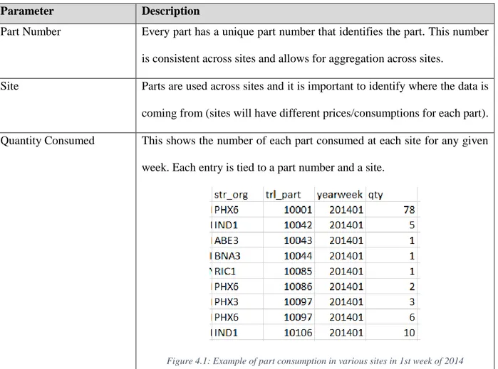
The table below shows the most relevant information that was extracted from EAM through SQL queries and how they were important to the overall model development process.
Parameter Description
Part Number Every part has a unique part number that identifies the part. This number is consistent across sites and allows for aggregation across sites.
Site Parts are used across sites and it is important to identify where the data is coming from (sites will have different prices/consumptions for each part). Quantity Consumed This shows the number of each part consumed at each site for any given
week. Each entry is tied to a part number and a site.
29
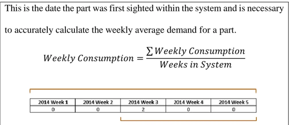
First Sighted Date This is the date the part was first sighted within the system and is necessary to accurately calculate the weekly average demand for a part.
𝑊𝑒𝑒𝑘𝑙𝑦 𝐶𝑜𝑛𝑠𝑢𝑚𝑝𝑡𝑖𝑜𝑛 =∑ 𝑊𝑒𝑒𝑘𝑙𝑦 𝐶𝑜𝑛𝑠𝑢𝑚𝑝𝑡𝑖𝑜𝑛 𝑊𝑒𝑒𝑘𝑠 𝑖𝑛 𝑆𝑦𝑠𝑡𝑒𝑚
For example, assume the table above shows the weekly demand for a part. If the demand is calculated as is, its demand would be 0.4 parts/week. However, if it is known that the part entered the system in Week 3, its average demand would be 0.66/week.
Store Min/Max Level and Current Quantity in Store
This shows the current min/max levels for every part in each site. This, together with the current quantity, is required for benchmarking the efficacy of the proposed inventory policy/pooling methodologies.
Lead Time / Avg. Price The average lead time and price is also available for any given part at a specific site. This is again required for quantifying proposed changes, but also required as a key parameter in applying the (R,Q) model.
Criticality The criticality of a part ranges from 1 to 3, and indicates how important a part is to a site (1 being the highest) and is similar to the A-B-C classification that Silver proposes for part prioritization.
Table 4.1: Parameters from SQL
4.2. Estimating Missing Data
Inventory models require specific inputs to generate results. For example, the (R,Q) model requires several parameters such as:
30
Usage data: Mean and standard deviation build a demand profile for the part.
Price: Affects EOQ and allows for quantification of savings
Lead Time: Dictates how much stock needs to be kept on hand (Cycle stock).
Criticality: Determines required service level for the part.
Any missing parameter would result in the model not being able to generate an optimal inventory stocking level for the part. Additionally, inaccuracies and missing data prevent the inventory model from being applies to all parts within the system. At present, only 57% of parts (in total monetary value) have sufficient data to allow for an implementation of an inventory model.
The following methods were employed to estimate the necessary parameters (where possible) and only parameters that could be estimated with a sufficient level of confidence were included within the study. This was able to improve the total parts included in the study from 57% to 67%, which still excluded approximately 33% of parts (in total monetary value). However, estimating parameters for the remaining parts could result in inaccurate values that would invalidate the entire model.
Although EAM provides each part in each site with its own parameters, a “common” parameter for each part has to be established for pooling purposes (i.e. a part must have one price within the system when pooled as opposed to having an individual price for each site). As the final goal of this project involves pooling, it makes sense to establish this common parameter and, if there is sufficient confidence in the “common” parameter, to apply that common parameter as the estimated data.
Criticality
Criticality values define the required service value for the inventory model. Due to the potential consequences of stockouts, if no parts within the network have an assigned criticality, the criticality for that part is assumed to be 1 (the highest criticality).
31
All parts take on the highest criticality assigned to the part across all sites. It is acknowledged that this may be overly conservative as sites with ten processing lines may have a low criticality for a part, whereas sites with only two lines may have the exact same part assigned a high criticality. However, due to the high service level requirements, this was chosen as the best compromise.
Lead Time
Lead times directly affect the inventory that has to be kept on hand due to its direct relationship with cycle stock. It is assumed that the bulk of the lead time comes from the manufacturer/supplier and not due to shipping. As such, for any given part, it is assumed that lead times will be fairly similar between sites.
All lead times of 0 are assumed to be missing data and will require estimation. An average is taken of all parts with non-zero lead time data. However, once an average is found, any parts with a lead time of +/- 1.282 SDs away from the mean is removed from the data (to eliminate potential outlier data), and a new average calculated. This mean is taken as the estimated lead time for that part and applied to all parts across all sites. In the event that there is no way of estimating a lead time for the part, it is assumed to be 4 weeks – the lead time for the vast majority of parts as shown from the distribution of parts below.
Figure 4.2: Lead Time Distribution for Parts Price
Prices affect the optimal ordering quantity (a cheaper price would result in a higher EOQ) and are vital for quantifying results. As parts are secured from different suppliers, parts will have different prices within the
32
system. Additionally, as these prices are input manually, they are also prone to errors (e.g. a $400 part may be input as $40,000) which could greatly skew recommendations. This was the area with the highest variation and risk of inaccuracies.
A common price, established through determining a mean/median price, helps to mitigate many of these problems. As before, it is assumed that although there are variations, the price for any given part is relatively similar across sites. Missing prices were estimated in three ways. These are presented based below in decreasing order of priority (i.e. the model will try to estimate prices using method 1 first when it encounters a missing price):
1) Preferred Supplier’s Price of Part (within EAM) 2) Average price of equivalent parts in other sites 3) Average price of that particular part class (e.g. roller)
Once all parts have an estimated price, the model identifies a common price for each part. As before, all prices of 0 are assumed to be missing data. At this point, the model then identifies the mean and median price for each part based on the remaining price data.
The model then overwrites each part with the “common” price – either the mean or the median price for each part. These data points are presented below. Pre-consolidation refers to the sum of prices before the prices were overwritten and is adjusted to be $200 million for privacy reasons. The median and mean prices were also adjusted accordingly, keeping the ratios constant.
Configuration Total Price of all Parts Ratio to Pre-Consolidation
Pre-Consolidation $200,000,000 1
Median $206,990,387 1.035
Mean $231,333,947 1.157
Table 4.2: Median vs Mean Price
In both cases, the median and mean both report higher prices than the pre-consolidation total. This suggests that many parts have under-reported prices within the system. An aggregation of the data shows many parts
33
have a price of $1, which is not unexpected given that the recorded price within EAM used to be of no importance to the overall ordering process.
It is also worth noting that the mean prices are much higher than median prices, which suggest the presence of large outlier prices skewing the data upwards (as opposed to median prices were effectively eliminates larger outliers). Although the specific data cannot be shared, it is worth noting that the number of parts that had heavily under-reported prices were consistent across both the mean and median price consolidation methods.
In further support of price consolidation, there were a significant number of parts whose individual prices were significantly higher/lower than the mean/median price. For example, approximately 1,500 parts had a reported cost than was <10% of the mean cost, and approximately 400 parts had a reported cost that was 10,000% higher than the median cost. This highlights the variability in price and why consolidation is required for comparison purposes (i.e. It is not realistic for one site to buy a part for $210, whereas another site purchases the same part for $10).
Based on the findings from this analysis, the median price was used as the “standard” price. It was found that most parts were accurately reported (with most actual prices ranging between ±10% of the median), but outliers were typically more than an order of magnitude off. As such, the median was used as it remains true to the pre-adjustment value, but eliminates outlier values (e.g. $1 parts or overly expensive parts) that would skew results in mean-based reporting.
Usage Data
Usage data is exceptionally important as it provides a demand profile for each part and determines how much inventory needs to be kept on-hand. Due to the importance of this data, average demands and standard deviations are not estimated. If a part does not have usage data, it is excluded from the analysis.
34
4.3. Improving Data Accuracy – Returns and Outliers
In order to further improve the accuracy of the model, it was necessary to address issues that could skew the results. Trending of data points identified two areas of concern– extreme outliers and returned parts.
Outliers are especially concerning due to the very sparse demand data for most parts. Unexpectedly, most spares are unused from week-to-week and weekly demand for most part has a mode of zero.
Figure 4.3: Sample Week-By-Week Demand for 3 Parts
The sparse demand profiles exacerbate the impact of outliers in demand data, particularly when the part has not been on the shelves for very long. Additionally, this means that average weekly demand numbers do not necessarily reflect the actual weekly consumption required when parts are actually used.
Returns
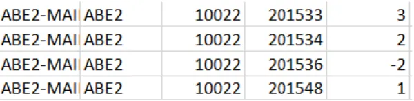
The data management software allows for unused spare parts to be “returned” to the available spares after it has been checked out. For example, if three parts were taken out for a job, but only two were used, the last part can be returned upon completion of the job. Any returns to the system are input as negative uses which replenishes inventory levels for that part as shown below (item receivals are recorded separately, so there is no risk of confusion).
Figure 4.4: Example of Negative Usage Data for Part 10022 in Site ABE2
Unfortunately, as seen above, these returns may not be identified until a few weeks later. If parts are checked out but returned in a different week, this will result in incorrect demand reporting. In order to address this, it was assumed that returns can only occur after a part is checked out. As such, all negative usages were
35
assumed to be cancelled out by previous positive usages (starting with the most recently checked out part and working backwards). For example, in the example above, the two negative usages in the 36th week of
2015 would cancel out the two parts “used” in the 34th week.
In order to prevent incorrect “return” entries from corrupting the data, it is assumed that if a return is not fully removed after four weeks of “backtracking”, there was a mistake in the quantity associated with the return, and any remaining amount to be returned is automatically deleted (with no other usages being deleted). This is able to correct the data to produce the cost chart as shown to the right below.
Figure 4.5: Consumption of Parts by Cost (Original vs Smoothed)
Although details on axis ticks were removed for data privacy reasons, it can be assumed that the lowest tick on the y axis corresponds to $0 total cost. Notice that the two negative spikes in ~weeks 38 and 41 have now been removed. Although this resulted in a negative spike in ~week 3, that negative spike was later found to be due to a negative price associated with a part in EAM (which was then removed from the dataset). The next section addresses how these outliers were identified and addressed.
Outliers
As highlighted by the previous section on estimating parameters, outliers present a significant risk to the accuracy of the model. This is exacerbated by the sparse demand data for most parts. Due to the size of the data (>1M data points), it was not feasible to investigate each data point. However, large outliers were identified by plotting the weekly consumption for parts and identifying large spikes in the data.
36
Plotting the weekly cost of parts consumption provided a way to identify abnormally high demand and high prices within the data as shown in the plots below. The plot on the left shows the original data. Each extreme point was individually and EAM admins were consulted when cases could not be immediately ruled out. For example, in the chart to the left, ~Week 40 of 2014 and ~Week 45 of 2016 show large spikes that warranted further attention. All unrealistic data points were removed which resulted in a much smoother chart as shown in the plot to the right, although spikes still do exist as part of normal operations.
Figure 4.6: Consumption of Parts by Cost (Before / After Adjustment)
Additionally, plots were also created for total parts consumed per week. This ensured that parts with high demand (but inaccurately low prices) were not missed. For example, the plot below helped to identify a large spike in demand on the 30th week of 2017 that would have been missed by evaluating cost alone.
37
4.4. Data Analysis
The above sections highlighted the data that was extracted from EAM, how missing data was estimated, and how outliers were identified and removed from the dataset. As mentioned in Section 4.1.1, the weekly demand statistics (average demand and standard deviation) could be calculated based on the consumption numbers and the known “first sighted” date of the part.
The dataset provides all the parameters needed to breakdown the data and identify key areas for improvement and answer high level questions that would impact the overall strategy regarding inventory.
4.4.1.
Aggregation of Data
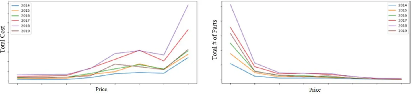
Although the analyses yielded useful data for prioritizing the inventory optimization methodology, they cannot be shared due to information that is confidential to Amazon. A small number of the data trends are presented below as examples to provide guidance for similar studies.
For example, Figure 4.8 below shows how the total cost and number of parts vary as the price of the parts increase. In this example, the data shows that the most expensive parts make up the largest proportion of cost, but make up a small proportion of the number of parts kept on-hand. Consequently, a larger focus was placed on ensuring that the more expensive marks were prioritized in the study.
38
4.4.2.
Managing Peak Seasons
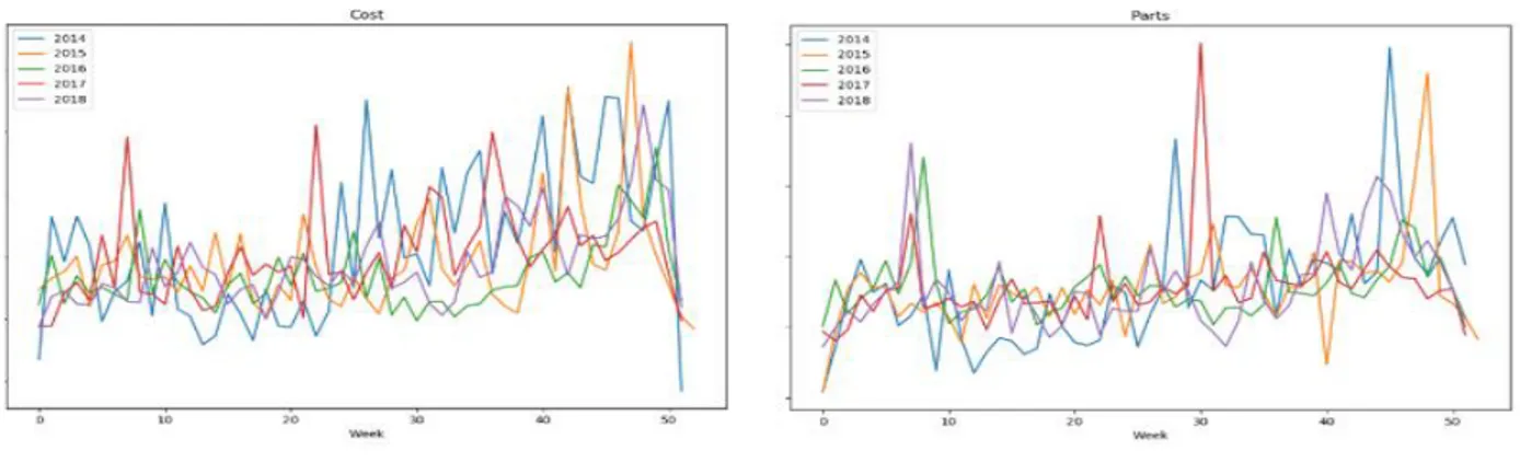
Amazon faces two peak seasons throughout the year – Prime Day and the Christmas holidays. These two peak periods typically result in higher traffic through FCs. One concern was the need to ensure higher reliability during this period, and that there may be an uptick in parts usage during and prior to peak seasons (whether due to preventative maintenance, or higher loads causing faster spare consumption). If there is a significant increase in part consumption, a separate inventory model (with higher quantities of spares) may be required for certain periods of the year to ensure an adequate service level during peak periods. This hypothesis was disproved by plotting an “adjusted” consumption chart that scales the parts consumption in each year so that the weekly demands can be better compared between years. Figure 4.9 suggests appears to be a peak in late February/early March, but when this peak was further examined in an unadjusted chart, the spike was found to be not significantly different enough to warrant a separate inventory policy.
Figure 4.9: Scale Adjusted Consumption Plots
The expectation is that any gains from implementing two separate models would be small enough that they are offset by the complications of managing two inventory models. Based on this, this paper did not further investigate the applications of having different inventory policies for different time periods as there was insufficient evidence that peak periods exhibited higher than average demand.
39
4.5. Summary
In order for established inventory models, such as the (R,Q) model, to be implemented, a large amount of data is required. In particular, the parameters of criticality, price, lead time and usage data are especially important. Although EAM makes a large amount of this data available, there were still instances where that data was not available. Efforts were made to estimate these parameters where possible, but is not always possible. For example, any attempts at estimating usage data would only make the data less accurate.
As data accuracy is exceptionally important in ensuring that the proposed inventory policy is fit for use, data was aggregated to identify any potential outliers which could then be manually verified and eliminated. Finally, the aggregation of data also allowed for big picture analysis of the data, and identified that demand for spare parts was largely random and did not follow any seasonal trends. This was an important insight as it meant that a separate inventory policy did not have to be developed for Amazon’s two peak periods throughout the year.
40
5. Inventory Model Development
Amazon’s current inventory management system does not make full use of the data that is available. As such, a single-stage inventory model is still likely to out-perform Amazon’s current system. The proposed (R,Q) inventory model was chosen on the assumption that Amazon’s supply chain involves an extended time horizon (i.e. multi-period model) and that parts will be reordered on a regular basis such that a continuous review period applies.
This chapter details how the (R,Q) model is applied within the Amazon context. Additionally, it goes into further detail regarding the background of the (R,Q) model by exploring its two building blocks - the Newsvendor and EOQ models.
5.1. Newsvendor Model
The newsvendor model is a single-period inventory model that ensures enough inventory is held to meet a required service level over a certain period of time (typically the lead time of the part). At a high level, the newsvendor model is made up of Cycle Stock (the expected amount of inventory required) and Safety Stock (the additional inventory carries to account for variations in demand).
The cycle stock and safety stock levels are a function of the various parameters that were determined in Chapter 4 and are shown below.
𝐶𝑦𝑐𝑙𝑒 𝑆𝑡𝑜𝑐𝑘: 𝑓(𝐴𝑣𝑒𝑟𝑎𝑔𝑒 𝐷𝑒𝑚𝑎𝑛𝑑, 𝐿𝑒𝑎𝑑 𝑇𝑖𝑚𝑒)
𝑆𝑎𝑓𝑒𝑡𝑦 𝑆𝑡𝑜𝑐𝑘: 𝑓(𝑆𝑡𝑎𝑛𝑑𝑎𝑟𝑑 𝐷𝑒𝑣𝑖𝑎𝑡𝑖𝑜𝑛 𝑜𝑓 𝐷𝑒𝑚𝑎𝑛𝑑, 𝑆𝑒𝑟𝑣𝑖𝑐𝑒 𝐿𝑒𝑣𝑒𝑙, 𝐿𝑒𝑎𝑑 𝑇𝑖𝑚𝑒, 𝐷𝑖𝑠𝑡𝑟𝑖𝑏𝑢𝑡𝑖𝑜𝑛 𝑇𝑦𝑝𝑒)
The consumption of spare parts may be hard to predict, but the statistical parameters determined before allow for the random variable to be modelled through a probability density function as shown in Figure 5.1 below. The cycle stock is represented by cumulative distribution to the left of the mean (µ). The safety stock is some additional stock held on hand to account for the potential demand variation to the right of the
41
mean. This serves as a buffer for higher than expected demand, and the specific amount of inventory held as safety stock will depend on the required service level.
The variable ‘k’ below represents the number of standard deviations from the mean required to hit the required service level. For example, a 95% service level will have a ‘k’ value of 1.65 (which corresponds to a cumulative distribution probability of 95%). The variable q* refers to the specific point on the distribution that results in the desired service level / cumulative probability.
Figure 5.1:Newsvendor Diagram
A traditional newsvendor model will determine the optimal ‘k’ value through the overage and underage model described in Chapter 2. However, due to Amazon’s strict MHE uptime requirements, the underage costs are considered to be significantly higher than the underage costs, and are not easily quantified.
Although Amazon would prefer a service level of 100%, it should be noted that this is statistically impossible, and would require an infinite number of parts. Instead, the required service levels were manually selected based on the parts’ criticalities. It should be acknowledged that this was a deliberate decision that was made to optimize for uptime, but may come at a potentially higher cost (than if the overage/underage method were used).
42
Criticality Service Level k Score
1 99.5% 2.58
2 99% 2.33
3 95% 1.65
Table 5.1: Criticality to Service Level Mapping
Based on this criticality, the amount of inventory for each part required on-hand can be calculated by applying the formula below based on each part’s individual parameters.
𝐼𝑛𝑣𝑒𝑛𝑡𝑜𝑟𝑦 𝑅𝑒𝑞𝑢𝑖𝑟𝑒𝑑 = 𝐶𝑦𝑐𝑙𝑒 𝑆𝑡𝑜𝑐𝑘 + 𝑆𝑎𝑓𝑒𝑡𝑦 𝑆𝑡𝑜𝑐𝑘 𝐼𝑛𝑣𝑒𝑛𝑡𝑜𝑟𝑦 𝑅𝑒𝑞𝑢𝑖𝑟𝑒𝑑 [𝑃𝑎𝑟𝑡𝑠] = ( µ [𝑃𝑎𝑟𝑡𝑠 𝑇𝑖𝑚𝑒] ∗ 𝐿𝑒𝑎𝑑 𝑇𝑖𝑚𝑒 [𝑇𝑖𝑚𝑒]) + (𝑘 ∗ 𝜎 [ 𝑃𝑎𝑟𝑡𝑠 𝑇𝑖𝑚𝑒] ∗ √𝐿𝑒𝑎𝑑 𝑇𝑖𝑚𝑒 [𝑇𝑖𝑚𝑒]) As evidenced above, the Newsvendor model requires an underlying distribution to build its recommended inventory (otherwise ‘k’ and σ do not exist). Although Figure 5.1 above uses a normal distribution for illustrative purposes, the stochastic nature of spare parts consumption may not follow a normal distribution.
5.1.1.
Potential Distribution Types
There are a number of distribution types typically used for Newsvendor models. Examples include the Normal distribution, the Poisson distribution, and the Negative Binomial distribution (but is not limited to these). The following sections details the benefits and complications that arise from each distribution type to establish a baseline for selecting a distribution type.
Normal Distribution
The Normal distribution is one of the most preferred distribution types due to its versatility and ease of application. The cumulative distribution for Normal distributions is given by
43
Where k represents the number of standard deviations away from the mean required to achieve the desired cumulative probability.
The Normal distribution is a continuous distribution that is bounded by [-∞,∞]. This results in several problems when applying the Normal distribution to inventory.
First, inventory is usually best modelled through discrete distributions (with count variables). However, this can be mitigated by rounding all partial inventories upwards (to be conservative). Additionally, Amazon FCs often use “partial” parts for certain consumables (e.g. length of conveyor belt) which discrete distributions will not be able to adequately deal with.
The second point of consideration is that inventory cannot be negative (i.e. it should be bounded by [0,∞]). However, by definition, average demand (µ) for a part must always be greater than zero which means that negative values will always fall to the left of the mean. As Amazon’s service levels (>95%) will always result in the required inventory being to the right of the mean, any negative values on the distribution curve can effectively be ignored.
Finally, although the Normal distribution may not perfectly map to the consumptions’ distributions, the large number of data entries enables the Central Limit Theorem to hold, which supports the applications of a Normal distribution.
Poisson Distribution
The Poisson distribution is a discrete distribution that typically works well for count data (i.e. non-negative integer data {0, 1, 2…}). The Poisson distribution is described by a single parameter (λ) where λ > 0. By definition, the mean of a Poisson distribution is equal to its variance:
𝑌 ~ 𝑃(λ = x) =𝑒
−λλx
𝑥! 𝐸(Y) = 𝑉𝑎𝑟(Y)
44
Additionally, the Poisson distribution models the sparse demand profile of spare parts quite well as it is very right-skewed with many data points at 0. Given that Poisson distributions are discrete distributions, the cumulative probability function is:
𝑃(𝑋 ≤ 𝑘) = ∑𝑒
−λλi
𝑖!
𝑘
𝑖=0
As such, q*, for a given service level (𝛼) is such that:
∑ 𝑒 −λλi 𝑖! 𝑞∗−1 𝑖=0 ≤ 𝛼 ≤ ∑𝑒 −λλi 𝑖! 𝑞∗ 𝑖=0
The Poisson is an especially good approximation when the data is under-dispersed (when the mean is less than, or equal to, the variance (i.e. (E(Y) ≤ Var(Y))). When the data is over-dispersed (i.e. (E(Y) > Var(Y)), the Negative Binomial Distribution becomes a better approximation. Based on the data available, there is a fairly even mix of over-dispersed and under-dispersed data, which makes it difficult to select between the two.
Count (n = 100,000+)
E(Y) < Var(Y) 27.2%
E(Y) = Var(Y) 13.3%
E(Y) > Var(Y) 59.5%
Table 5.2: Mean vs Variance Distribution of Dataset
Negative Binomial Distribution
The Negative Binomial Distribution is similar to the Poisson distribution, but works better with over-dispersed data. Unfortunately, the data is a fairly balanced mix of over-over-dispersed and under-over-dispersed data (which would be better served by a Poisson distribution). As such, there is no clear way of choosing one distribution over the other.