HAL Id: inria-00397689
https://hal.inria.fr/inria-00397689
Submitted on 23 Jun 2009
HAL is a multi-disciplinary open access
archive for the deposit and dissemination of
sci-entific research documents, whether they are
pub-lished or not. The documents may come from
teaching and research institutions in France or
abroad, or from public or private research centers.
L’archive ouverte pluridisciplinaire HAL, est
destinée au dépôt et à la diffusion de documents
scientifiques de niveau recherche, publiés ou non,
émanant des établissements d’enseignement et de
recherche français ou étrangers, des laboratoires
publics ou privés.
On the relation between sized-types based termination
and semantic labelling
Frédéric Blanqui, Cody Roux
To cite this version:
Frédéric Blanqui, Cody Roux. On the relation between sized-types based termination and semantic
labelling. 18th EACSL Annual Conference on Computer Science Logic - CSL 09, Sep 2009, Coimbra,
Portugal. �inria-00397689�
On the relation between sized-types based
termination and semantic labelling
Fr´ed´eric Blanqui1 and Cody Roux2(INRIA)
1 FIT 3-604, Tsinghua University, Haidian District, Beijing 100084, China, [email protected]
2 LORIA⋆⋆
, Pareo team, Campus Scientifique, BP 239, 54506 Vandoeuvre-l`es-Nancy, Cedex, France, [email protected]
Abstract. We investigate the relationship between two independently developed termination techniques. On the one hand, sized-types based termination (SBT) uses types annotated with size expressions and Gi-rard’s reducibility candidates, and applies on systems using construc-tor matching only. On the other hand, semantic labelling transforms a rewrite system by annotating each function symbol with the semantics of its arguments, and applies to any rewrite system.
First, we introduce a simplified version of SBT for the simply-typed lambda-calculus. Then, we give new proofs of the correctness of SBT using semantic labelling, both in the first and in the higher-order case. As a consequence, we show that SBT can be extended to systems using matching on defined symbols (e.g. associative functions).
1
Introduction
Sized types were independently introduced by Hughes, Pareto and Sabry [16] and Gim´enez [11], and were extended to richer type systems, to rewriting and to richer size annotations by various researchers [21,1,2,5,7].
Sized types are types annotated with size expressions. For instance, if T is the type of binary trees then, for each a ∈ N, a type Ta is introduced to type
the trees of height smaller or equal to a. In the general case, the size is some ordinal related to the interpretation of types in Girard’s reducibility candidates [12]. However, as suggested in [5], other notions of sizes may be interesting.
These size annotations can then be used to prove the termination of functions by checking that the size of arguments decreases along recursive calls, but this applies to functions defined by using matching on constructor terms only.
At about the same time, semantic labelling was introduced for first-order systems by Zantema [22]. It received a lot of attention in the last years and was recently extended to the higher-order case by Hamana [13].
In contrast with SBT, semantic labelling is not a termination criterion but transforms a system into another one whose termination is equivalent and hope-fully simpler to prove. The transformation consists in annotating function sym-bols with the semantics of their arguments in some model of the rewrite system.
⋆⋆
Finding a model may of course be difficult. We will see that the notion of size used in SBT provides such a model.
In this paper, we study the relationship between these two methods. In par-ticular, we give a new proof of the correctness of SBT using semantic labelling. This will enable us to extend SBT to systems using matching on defined symbols. Outline. Section 2 introduces our notations. Section 3 explains what SBT is and Section 4 introduces a simplified version of it. To ease the understanding of the paper, we first present the first-order case which already contains the main ideas, and then consider the higher-order case which requires more knowledge. Hence, in Section 5 (resp. 7), we recall what is semantic labelling in the first (resp. higher) order case and show in Section 6 (resp. 8) that SBT is an instance of it. For lack of space, some proofs are given in the Appendices of [8].
2
Preliminaries
First-order terms. A signature F is made of a set Fn of function symbols of
arity n for each n ∈ N. Let F be the set of all function symbols. Given a set X
of variables, the set of first-order terms T (F , X ) is defined as usual: X ⊆ T ; if f∈ Fn and t is a sequence t1, . . . , tn∈ T of length n = |t|, then f(t) ∈ T .
An F -algebra M is given by a set M and, for each symbol f ∈ Fn, a function
fM: Mn→ M . Given a valuation µ : X → M , the interpretation of a term t is
defined as follows: [[x]]µ = µ(x) and [[f(t1, . . . , tn)]]µ = fM([[t1]]µ, . . . , [[tn]]µ).
Positions are words on N. We denote by ε the empty word and by p · q or pq
the concatenation of p and q. Given a term t, we denote by t|p the subterm of
t at position p, and by t[u]p the replacement of this subterm by u. Let Pos(f, t)
be the set of the positions of the occurrences of f in t.
Higher-order terms. The set of (simple) types is T = T (Σ) where Σ0= B
is a set of base types, Σ2= {⇒} and Σn= ∅ otherwise. The sets of positive and
negative positions in a type are inductively defined as follows:
– Pos+(B) = ε and Pos−(B) = ∅ for each B ∈ B,
– Posδ(T ⇒ U ) = 1 · Pos−δ(T ) ∪ 2 · Posδ(U ) where −− = + and −+ = −. Let X be an infinite set of variables. A typing environment Γ is a map from a finite subset of X to T. For each type T , we assume given a set FT of
function symbols of type T . The sets ΛT(Γ ) of terms of type T in Γ are defined
as usual: FT ⊆ ΛT(Γ ); if (x, T ) ∈ Γ then x ∈ ΛT(Γ ); if t ∈ ΛU(Γ, x : T ), then
λxTt ∈ Λ
T⇒U(Γ ); if t ∈ ΛU⇒V(Γ ) and u ∈ ΛU(Γ ), then tu ∈ ΛV(Γ ).
Let F (resp. Λ) be the set of all function symbols (resp. terms). Let X (t) be the set of free variables of t. A substitution σ is a map from a finite subset of X to Λ. We denote by (u
x) the substitution mapping x to u, and by tσ the
application of σ to t. A term t β-rewrites to a term u, written t →β u, if there
is p ∈ Pos(t) such that t|p= (λxTv)w and u = t[vxw]p.
A rewrite rule is a pair of terms l → r of the same type such that X (r) ⊆ X (l). A rewrite system is a set R of rewrite rules. A term t rewrites to a term u, written t →Ru, if there is p ∈ Pos(t), l → r ∈ R and σ such that t|p= lσ and u = t[rσ]p.
Constructor systems. A function symbol f is either a constructor symbol if no rule left-hand side is headed by f, or a defined symbol otherwise. A pattern is a variable or a term of the form ct with c a constructor symbol and t patterns. A rewrite system is constructor if every rule is of the form fl → r with l patterns. As usual, we assume that constructors form a valid inductive structure [6], that is, there is a well-founded quasi-ordering ≤B on B such that, for each base
type B, constructor c : T ⇒ B and base type C occuring at position p in Ti,
either C <BBor C ≃BBand p ∈ Pos+(Ti). Mendler indeed showed that invalid
inductive structures lead to non-termination [18].
Given a constructor c : T ⇒ B, let Ind(c) be the set of integers i such that Ti
contains a base type C ≃BB. A constructor c with Ind(c) 6= ∅ is said recursive.
A constructor c : T ⇒ B is strictly-positive if, for each i, either no base type equivalent to B occurs in Ti, or Ti is of the form U ⇒ C with C ≃B Band no
base type equivalent to B occuring in U .
SBT applies to constructor systems only. By using semantic labelling, we will prove that it can also be applied to some non-constructor systems.
3
Sized-types based termination
We now present a simplified version of the termination criterion introduced in [5], where the first author considers rewrite systems on terms of the Calculus of Algebraic Constructions, a complex type system with polymorphic and depen-dent types. Here, we restrict our attention to simply-typed λ-terms since there is no extension of semantic labelling to polymorphic and dependent types yet.
This termination criterion is based on the semantics of types in reducibility candidates [12]. An arrow type T ⇒ U is interpreted by the set [[T ⇒ U ]] = {v ∈ T | ∀t ∈ [[T ]], vt ∈ [[U ]]}. A base type B is interpreted by the fixpoint [[B]] of the monotonic function FB(X) = {v ∈ SN | ∀ constructor c : T ⇒ B, ∀t, ∀i ∈
Ind(c), v →∗ ct⇒ t
i ∈ [[Ti]]B7→X} on the lattice of reducibility candidates that
is complete for set inclusion [6]. This fixpoint, defined by induction on the well-founded quasi-ordering ≤Bon base types, can be reached by transfinite iteration
of FB up to some limit ordinal ωB strictly smaller than the first uncountable
ordinal A. This provides us with the following notion of size: the size of a term t ∈ [[B]] is the smallest ordinal oB(t) = a < A such that t ∈ FBa(⊥), where ⊥
is the smallest element of the lattice and Fa
B is the function obtained after a
transfinite iterations of FB.
This notion of size, which corresponds to the tree height for patterns, has the following properties: it is well-founded; the size of a pattern is strictly bigger than the size of its subterms; if t → t′ then the size of t′ is smaller than (since
→ may be non confluent) or equal to the size of t.
SBT consists then in providing a way to syntactically represent the sizes of terms and, given for each function symbol an annotation describing how the size of its output is related to the sizes of its inputs, check that some measure on the sizes of its arguments decreases in each recursive call.
Size algebra. Sizes are represented and compared by using a first-order term algebra A = T (Σ, X ) equipped with an ordering ≤A such that:
– <Ais stable by substitution;
– (A, <A), where <A is the usual ordering on ordinals, is a model of (A, <A):
• every symbol h ∈ Σn is interpreted by a function hA: An → A;
• if a <Ab then [[a]]µ <A[[b]]µ for each µ : X → A.
To denote a size that cannot be expressed in A (or a size that we do not care about), Σ is extended with a (biggest) nullary element ∞. Let A be the extended term algebra in which all terms containing ∞ are identified, <A = <A∪ {(a, ∞) | a ∈ A} and ≤A= ≤A∪ {(a, ∞) | a ∈ A}. Note that such an
ex-tension is often used in domain theory but with a least element instead. Annotated types. The set of base types is now all the expressions Ba such
that B ∈ B and a ∈ A. The interpretation of B∞ (also written B) is [[B]] and,
given a ∈ A, the interpretation of Ba wrt a size valuation µ : X → A is the set
of terms in [[B]] whose size is smaller or equal to [[a]]µ: [[Ba]]µ = F[[a]]µ B (⊥).
Hence, we assume that every symbol f ∈ F is given an annotated type τA f
whose size variables, like type variables in ML, are implicitly universally quan-tified and can be instantiated by any size expression. Hence the typing rule for symbols in Figure 1 allows any size substitution ϕ to be applied to τfA. Subtyping
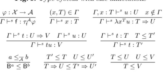
naturally follows from the interpretation of types and the ordering on A. Fig. 1. Type system with size annotations
ϕ : X → A Γ ⊢sf: τA f ϕ (x, T ) ∈ Γ Γ ⊢sx : T Γ, x : T ⊢s u : U x /∈ Γ Γ ⊢sλxTu : T ⇒ U Γ ⊢s t : U ⇒ V Γ ⊢s u : U Γ ⊢stu : V Γ ⊢s t : T T ≤ T′ Γ ⊢st : T′ a ≤Ab Ba≤ Bb T′ ≤ T U ≤ U′ T ⇒ U ≤ T′⇒ U′ T ≤ U U ≤ V T ≤ V
Definition 1. Given a type T , let T∞be the type obtained by annotating every
base type with ∞, and annotα
B(T ) be the type obtained by annotating every base
type C ≃B Bwith α, and every base type C 6≃B Bwith ∞. Conversely, given an
annotated type T , let |T | be the type obtained by removing all annotations.
Note that, in constrast to types, terms are unchanged: in λxTu, T = T∞.
Given a size symbol h ∈ Σ, let Mon+(h) (resp. Mon−(h)) be the sets of integers i such that h is monotonic (resp. anti-monotonic) in its i-th argument. The sets of positive and negative positions in an annotated type are:
– Pos−(Ba) = 0 · Pos−(a) and Pos+(Ba) = {ε} ∪ 0 · Pos+(a),
To ease the expression of termination conditions, for every defined symbol f, τA
f is assumed to be of the form P ⇒ B
αf ⇒ BfA(αf) with |τA
f | = τf, X (P ) = ∅
and X (fA(α
f)) ⊆ {αf} where αf are pairwise distinct variables. The arguments
of type B are the ones whose size will be taken into account for proving termi-nation. The arguments of type P are parameters and every rule defining f must be of the form fpl → r with p ∈ X , |p| = |P | and |l| = |B|.
Moreover, the annotated type of a constructor c : T1. . . Tn⇒ B is:
τcA= annotαB(T1) ⇒ . . . ⇒ annotαB(Tn) ⇒ Bc
A
(α)
with cA(α) = ∞ if c is non-recursive, and cA(α) = s(α) otherwise, where s is a monotonic unary symbol interpreted as the ordinal successor and such that a <As(a) for each a.
Termination criterion. We assume given a well-founded quasi-ordering ≥F on F and, for each function symbol f :s T ⇒ Bαf ⇒ Bf
A
(αf) and set X ∈ {A, A}, an ordered domain (DX
f , <Xf ) and a function ζfX : X|αf| → DfX
compatible with ≃F (i.e. |αf| = |αg|, DXf = DgX, <Xf = <Xg and ζfX = ζgX
whenever f ≃F g) and such that >Af is well-founded and ζ A f ([[a]]µ) < A f ζ A f ([[b]]µ) whenever ζA f (a) <Af ζfA(b) and µ : X → A.
Usual domains are Anordered lexicographically, or the multisets on A ordered
with the multiset extension of >A.
Theorem 1 ([5]). Let R be a constructor system. The relation →β ∪ →R
terminates if, for each defined f :s P ⇒ Bα ⇒ BfA
(α) and rule fpl → r ∈ R,
there is an environment Γ and a size substitution (a
α) such that:
– pattern condition: for each θ, if pθ ∈ [[P ]] and lθ ∈ [[B]] then there is ν such
that, for each (x, T ) ∈ Γ , xθ ∈ [[T ]]ν and [[a]]ν ≤ o B(lθ); – argument decreasingness: Γ ⊢s far : Bf A (a) where ⊢ fais defined in Figure 2;
– size annotations monotonicity: Pos(α, fA(α)) ⊆ Pos+(fA(α)).
The termination criterion introduced in [5] is not expressed exactly like this. The pattern condition is replaced by syntactic conditions implying the pattern condition, but the termination proof is explicitly based on the pattern condition. This condition means that a is a valid representation of the size of l, whatever the instantiation of the variables of l is, and thus that any recursive call with arguments of size smaller than a is admissible. The existence of such a valid syntactic representation depends on l and the size annotations of constructors. With the chosen annotations, the condition is not satisfied by some patterns (whose type admits elements of size bigger than ω, Appendix A). This suggests to use a more precise annotation for constructors.
The expressive power of the criterion depends on A. Taking the size algebra A reduced to the successor symbol s (the decidability of which is proved in [3]) is sufficient to handle every primitive recursive function. As an example, consider the recursor recT : O ⇒ T ⇒ (O ⇒ T ) ⇒ ((N ⇒ O) ⇒ (N ⇒ T ) ⇒ T ) ⇒ T
on the type O of Brouwer’s ordinals whose constructors are 0 : O, s : Oα⇒ Osα
and lim : (N ⇒ Oα) ⇒ Osα, where N is the type of natural numbers whose
Fig. 2. Computability closure g<Ff, ψ : X → A Γ ⊢s fa g: τ A g ψ
+ variable, abstraction, application and subtyping rules of Fig. 1
g≃F f g:s U ⇒ Cβ⇒ CgA(β) Γ ⊢s fau: U Γ ⊢ s fam: Bb ζ A f (b) < A f ζ A f (a) Γ ⊢s fagum: Cg A(b) rec0uvw → u rec(sx)uvw → vx(recxuvw) rec(limf )uvw → wf (λnrec(f n)uvw)
For instance, with f : N ⇒ Oα, we have limf : Osα, f n : Oαand sα > Aα.
An example of non-simply terminating system satisfying the criterion is the following system defining a division function / : Nα ⇒ N ⇒ Nα by using a
subtraction function − : Nα⇒ N ⇒ Nα. −x0 → x −0x → 0 −(sx)(sy) → −xy /0x → 0 /(sx)y → s(/(−xy)y) Indeed, with x : Nx, we have sx : Nsx, −xy : Nx and sx >
Ax.
4
Annotating constructor types with a max symbol
In this section, we simplify the previous termination criterion by annotating constructor types in an algebra made of the following symbols:
– 0 ∈ Σ0interpreted as the ordinal 0;
– s ∈ Σ1interpreted as the successor ordinal;
– max ∈ Σ2 interpreted as the max on ordinals.
For the annotated type of a constructor c : T1. . . Tn⇒ B, we now take:
τcA= annotαB1(T1) ⇒ . . . ⇒ annot αn
B (Tn) ⇒ B
cA(α1,...,αn)
with α distinct variables, cA(α) = 0 if c is non-recursive, and cA(α) = s(max(αi|
i ∈ Ind(c))) otherwise, where max(α1, . . . , αk+1) = max(α1, max(α2, . . . , αk+1))
and max(α1) = α1.
This does not affect the correctness of Theorem 1 since, in this case too, one can prove that constructors are computable: c ∈ [[τA
c ]]µ for each µ.
Moreover, now, both constructors and defined symbols have a type of the form annotα1
B1(T1) ⇒ . . . ⇒ annot
αn
Bn(Tn) ⇒ B
fA(α) with α distinct variables.
This means that a constructor can be applied to any sequence of arguments without having to use subtyping. Indeed, previously, not all constructor ap-plications were possible (take cxy with c : Bα ⇒ Bα ⇒ bsα, x : Bx and
y : By) and some constructor applications required subtyping (take cx(dx) with
We can therefore postpone subtyping after typing without losing much ex-pressive power . It follows that every term has a most general type given by a simplified version of the type inference system ⊢i of [3] using unification only
(see Appendix B).
Moreover, the pattern and monotonicity conditions can always be satisfied by defining, for each symbol f :sP ⇒ Bα⇒ U and rule fpl → r ∈ R, a as σ(l)
where σ(x) = x and σ(ct) = cA(σ(t)), and Γ as the set of pairs (x, T ) such that
x ∈ X (fpl) and T is: – Pi if x = pi,
– Bx
i if x = li,
– annotx
Bi(T ) if cuxv is a subterm of li and c : U ⇒ T ⇒ V ⇒ C.
Note that, if Γ ⊢ t : T and t is a non-variable pattern then there is a base type B such that Γ ⊢it : Bσ(t). So, σ(t) is the most general size of t.
Theorem 2. Let R be a constructor system. The relation →β∪ →Rterminates
if, for each f :sP ⇒ Bα⇒ BfA(α) and rule fpl → r ∈ R, we have:
– argument decreasingness: Γ ⊢i
far : Ba and a ≤AfA(a) where Γ and a = σ(l)
are defined just before and ⊢i
fais the type inference system ⊢i[3] (see Appendix
B) with function applications restricted as in Figure 2.
The proof is given in Appendix C. In the following, we say that R SB-terminates if R satisfies the conditions of Theorem 2.
5
First-order semantic labelling
Semantic labelling is a transformation technique introduced by Hans Zantema for proving the termination of first-order rewrite systems [22]. It consists in labelling function symbols by using some model of the rewrite system.
Let F be a first-order signature and M be an F -algebra equipped with a partial order ≤M. For each f ∈ Fn, we assume given a non-empty poset (Sf, ≤f)
and a labelling function πf : Mn → Sf. Then, let F be the signature such that
Fn = {fa| f ∈ Fn, a ∈ Sf}.
The labelling of a term wrt a valuation µ : X → M is defined as follows: labµ(x) = x and labµ(f(t
1, . . . , tn)) = fπf([[t1]]µ,...,[[tn]]µ)(lab
µ(t
1), . . . , labµ(tn)).
The fundamental theorem of semantic labelling is then:
Theorem 3 ([22]). Given a rewrite system R, an ordered F -algebra (M, ≤M)
and a labelling system (Sf, ≤
f, πf)f∈F, the relation →R terminates if:
1. M is a quasi-model of R, that is:
– for each rule l → r ∈ R and valuation µ : X → M , [[l]]µ ≥M[[r]]µ,
– for each f ∈ F, fM is monotonic; 2. for each f ∈ F, πf is monotonic;
3. the relation →lab(R)∪Decr terminates where:
lab(R) = {labµ(l) → labµ(r) | l → r ∈ R, µ : X → M },
Decr = {fa(x1, . . . , xn) → fb(x1, . . . , xn) | f ∈ F, a >f b}.
For instance, by taking M = N, 0M= 0, sM(x) = x + 1, −M(x, y) = x and
/M(x, y) = x, and by labelling − and / by the semantics of their first argument,
we get the following infinite system which is easily proved terminating: −ix0 → x (i ∈ N)
−00x → 0
−i+1(sx)(sy) → −ixy (i ∈ N)
/00x → 0
/i+1(sx)y → s(/i(−ixy)y) (i ∈ N)
6
First-order case
The reader may have already noticed some similarity between semantic labelling and size annotations. We here render it more explicit by giving a new proof of the correctness of SB-termination using semantic labelling.
In the first-order case, the interpretation of a base type does not require transfinite iteration: all sizes are smaller than ω and A = N [6]. Moreover, by taking Γ (x) = Bx for each x of type B, every term t has a most general size
σ(t) given by its most general type: Γ ⊢it : Cσ(t). This function σ extends to all
terms the function σ defined in the previous section by taking σ(f(t1, . . . , tn)) =
fA(σ(t1), . . . , σ(tn)) for each defined symbol f.
Theorem 4. SB-termination implies termination if:
– R is finitely branching and the set of constructors of each type B is finite; – for each defined symbol f, fAand ζA
f are monotonic.
Proof. For the interpretation domain, we take M = A = N which has a structure
of poset with ≤M=≤A=≤N.
If fA is not the constant function equal to ∞ (fA 6= ∞ for short), which is the case of constructors, then let fM(a) = [[fA(α)]]µ where αµ = a.
When fA = ∞, we proceed in a way similar to predictive labelling [15], a
variant of semantic labelling where only the semantics of usable symbols need to be given when M is a ⊔-algebra (all finite subsets of M have a lub wrt ≤M),
which is the case of N. Here, the notions of usable symbols and rules are not necessary and a semantics can be given to all symbols thanks to the strong assumptions of SB-termination. Let (f, x) >A (g, y) if f >F g or f ≃F g and ζfA(x) > A f ζ A
f (y). The relation
>A
is well-founded since the relations >F and >Af are well-founded. We then
define fM by induction on >A
by taking fM(a) = max({0} ∪ {[[r]]µ | fl → r ∈
R, µ : X → A, [[l]]µ ≤ a}). This function is well defined since:
– For each subterm gm in r, (f, σ(l)) >A (g, σ(m)). Assume that f ≃ F g.
Then, σ(l) >Aσ(m). Hence, for each symbol f occuring in l or m, fA6= ∞.
– The set {(fl → r, µ) | fl → r ∈ R, [[l]]µ ≤ a} is finite. Indeed, since l are patterns and constructors are interpreted by monotonic and strictly extensive functions (i.e. cA(α) ≥
A s(max(αi | i ∈ Ind(c)))), [[l]]µ is strictly monotonic
wrt µ and the height of l. We cannot have an infinite set of l’s of bounded height since, for each base type B, the set of constructors of type B is finite. And we cannot have an infinite set of r’s since R is finitely branching.
We do not label the constructors, i.e. we take any singleton set for Sc and
the unique (constant) function from Mn to Sc for π
c. For any other symbol f,
we take Sf = DA
f which is well-founded wrt >f, and πf = ζfA.
1. M is a quasi-model of R:
– Let f :s P ⇒ Bα ⇒ BfA(α), l → r ∈ R with l = fpl, and µ : X →
M . We have [[l]]µ = fM(a) where a = [[l]]µ. If fA = ∞, then fM(a) = max({0} ∪ {[[r]]µ | fl → r ∈ R, µ : X → A, [[l]]µ ≤ a}) and [[l]]µ ≥ [[r]]µ. Assume now that fA 6= ∞. Since Γ ⊢
fa r :i Ba and a ≤A fA(a), we have
σ(r) = a ≤A fA(a) = σ(l) where a = σ(l). By definition of Γ and σ, for each i, ai6= ∞ (a 6= ∞ for short). Therefore, σ(l) 6= ∞ and σ(r) ≤Aσ(l).
Hence, [[l]]µ = σ(l)µ ≤Aσ(r)µ = [[r]]µ since ≤Ais a model of ≤A.
– If f is a non-recursive constructor, then fM(a) = 0 is monotonic. If f is a
recursive constructor, then fM(a) = sup{a
i| i ∈ Ind(c)} + 1 is monotonic.
If fA 6= ∞, then fM(a) = [[fA(α)]]µ where αµ = a is monotonic since fA
is monotonic by assumption. Finally, if fA= ∞, then fM(a) = max({0} ∪
{[[r]]µ | fl → r ∈ R, µ : X → A, [[l]]µ ≤ a}) is monotonic.
2. If f is a defined symbol, then the function πf is monotonic by assumption. If
f is a constructor, then the constant function πf is monotonic too.
3. We now prove that →lab(R)∪Decr is precedence-terminating (PT), i.e. there
is a well-founded relation > on symbols such that, for each rule fl → r ∈ lab(R) ∪ Decr, every symbol occurring in r is strictly smaller than f [19]. Let ga < fb if g <F f or g ≃F f and a <Af b. The relation > is well-founded
since both >F and >Af are well-founded.
Decr is clearly PT wrt >. Let now fl → r ∈ R, µ : X → M and gt be a subterm of r. The label of f is a = πf([[l]]µ) = ζfA([[σ(l)]]µ) and the label of g
is b = ζA
f ([[σ(m)]]µ). By assumption, (f, l) >A(g, m). Therefore, a > A f b. ⊓⊔
It is interesting to note that we could also have taken M = A, assuming that <Af is stable by substitution (ζfA(aθ) <Af ζfA(bθ) whenever ζfA(a) <Af ζfA(b)). The system labelled with A is a syntactic approximation of the system labelled with A. Although less powerful a priori, it may be interesting since it provides a finite representation of the infinite A-labelled system.
Finally, we see from the proof that the system does not need to be construc-tor:
Theorem 5. Theorem 4 holds for any (non-constructor) system R such that,
for each rule fl → r ∈ R with fA= ∞ and subterm gm in l:
– gAis monotonic and strictly extensive: gA(α) ≥
– if gA= ∞, then g <
F f or g ≃F f and ζfA(σ(m)) <Af ζfA(σ(l)).
Example: assuming that A is the ⇒-type constructor, then the expression Fnuv represents the set of n-ary functions from u to v.
+0y → y +(sx)y → s(+xy) +(+xy)z → +x(+yz) F0uv → v F(sx)uv → Au(Fxuv) F(+xy)uv → Fxu(Fyuv)
Take +A(x, y) = ζ+(x, y) = a = 2x + y + 1, FA= ∞ and ζF(x, u, v) = x. The
interpretation of FMis well-defined since x < a and y < a. The labelled system that we obtain (where b = 2y + z + 1) is precedence-terminating:
+y+10y → y
+a+2(sx)y → s(+axy)
+2a+z+1(+axy)z → +2x+b+1x(+byz)
F00uv → v
Fx+1(sx)uv → Au(Fxxuv)
Fa(+axy)uv → Fxxu(Fyyuv)
7
Higher-order semantic labelling
Semantic labelling was extended by Hamana [13] to second-order Inductive Data Type Systems (IDTSs) with higher-order pattern-matching [4]. IDTSs are a typed version of Klop’s Combinatory Reduction Systems (CRSs) [17] whose cat-egorical semantics based on binding algebras and F -monoids [10] is studied by the same author and proved complete for termination [14].
The fundamental theorem of higher-order semantic labelling can be stated exactly as in the first-order case, but the notion of model is more involved.
CRSs and IDTSs. In CRSs, function symbols have a fixed arity.
Meta-terms extend Meta-terms with the application Z(t1, . . . , tn) of a meta-variable Z ∈ Z
of arity n to n meta-terms t1, . . . , tn.
An assignment θ maps every meta-variable of arity n to a term of the form λx1..λxnt. Its application to a meta-term t, written tθ, is defined as follows:
– xθ = x, (λxt)θ = λx(tθ) and f(t1, . . . , tn)θ = f(t1θ, . . . , tnθ);
– for θ(Z) = λx1..λxnt, Z(t1, . . . , tn)θ = t{x17→ t1θ, . . . , xn7→ tnθ}.
A rule is a pair of meta-terms l → r such that l is a higher-order pattern [20]. In IDTSs, variables, meta-variables and symbols are equipped with types over a discrete category B of base types. However, Hamana only considers structural
meta-terms where abstractions only appear as arguments of a function symbol,
variables are restricted to base types, meta-variables to first-order types and function symbols to second-order types. But, as already noticed by Hamana, this is sufficient to handle any rewrite system (see Section 8). Let IZ
B(Γ ) be the
set of structural meta-terms of type B in Γ whose meta-variables are in Z. Models. The key idea of binding algebras [10] is to interpret variables by natural numbers using De Bruijn levels , and to handle bound variables by extending the interpretation to typing environments.
Let F be the category whose objects are the finite cardinals and whose arrows from n to p are all the functions from n to p. Let E be the (slice) category of typing environments whose objects are the maps Γ : n → B and whose arrows from Γ : n → B to ∆ : p → B are the functions ρ : n → p such that Γ = ∆ ◦ ρ.
Given Γ : n → B, let Γ + B : n + 1 → B be the environment such that (Γ + B)(n) = B and (Γ + B)(k) = Γ (k) if k < n.
Let M be the functor category (SetE)B. An object of M (presheaf) is given by a family of sets MB(Γ ) for every base type B and environment Γ and, for every
base type B and arrow f : Γ → ∆, a function MB(f ) : MB(Γ ) → MB(∆) such
that MB(idΓ) = idMB(Γ )and MB(f ◦g) = MB(f )◦MB(g). An arrow α : M → N in M is a natural transformation, i.e. a family of functions αB(Γ ) : MB(Γ ) →
NB(Γ ) such that, for each ρ : Γ → ∆, αB(∆) ◦ MB(ρ) = NB(ρ) ◦ αB(Γ ).
Given M ∈ M, Γ ∈ E and B ∈ B, let upB
Γ(M ) : M (Γ ) → M (Γ + B) be the
arrow equal to M (idΓ + 0∆) where 0∆ is the unique morphism from 0 to ∆.
An X + F -algebra M is given by a presheaf M ∈ M, an interpretation of variables ι : X → M and, for every symbol f : (B1 ⇒ B1) ⇒ . . . ⇒ (Bn ⇒
Bn) ⇒ B and environment Γ , an arrow fM(Γ ) :Qni=1MBi(Γ + Bi) → MB(Γ ). The category M forms a monoidal category with unit X and product • such that (M • N )B(Γ ) is the set of equivalence classes on the set of pairs (t, u) with
t ∈ MB(∆) and ui ∈ N∆(i)(Γ ) for some ∆, modulo the equivalence relation
∼ such that (t, u) ∼ (t′, u′) if there is ρ : ∆ → ∆′ for which t ∈ M B(∆),
t′= M
B(ρ)(t) and u′ρ(i)= ui.
To interpret substitutions, M must be an F -monoid, i.e. a monoid (M, µ : M2→ M ) compatible with the structure of F-algebra [13] (see Appendix E).
The presheaf I∅ equipped with the product µ
B(Γ )(t, u) = t{i 7→ ui}
(simul-taneous substitution) is initial in the category of F -monoids [14]. Hence, for each F-monoid M, there is a unique morphism !M: I∅→ M .
Labelling. As in the first-order case, for each f : (B1⇒ B1) ⇒ . . . ⇒ (Bn⇒
Bn) ⇒ B, we assume given a non-empty poset (Sf, ≤f) for labels and a labelling
function πf(Γ ) :Qni=1MBi(Γ + Bi) → S
f. LetF
n= {fa | f ∈ Fn, a ∈ Sf}. Note
that the set of labelled meta-terms has a structure of F -monoid [13].
The labelling of a meta-term wrt a valuation θ : Z → I∅is defined as follows:
– labθ B(Γ )(x) = x; – labθ B(Γ )(Z(t1, . . . , tn)) = Z(labθB(Γ )(t1), . . . , labθB(Γ )(tn)); – for f : (B1⇒ B1) ⇒ . . . ⇒ (Bn⇒ Bn) ⇒ B and Γi= Γ, xi: Bi, labθ B(Γ )(f(λx1t1, . . . , λxntn)) = fa(labθB1(Γ1)(t1), . . . , lab θ Bn(Γn)(tn)) where a = πf(!MB1(Γ1)(t1θ), . . . , ! M Bn(Γn)(tnθ)).
We can now state Hamana’s theorem for higher-order semantic labelling. Theorem 6 ([13]). Given a structural IDTS R, an ordered F -algebra (M, ≤M)
and a labelling system (Sf, ≤
f, πf)f∈F, the relation →R terminates if:
1. (M, ≤M) is a quasi-model of R, that is:
– for each l → r : T ∈ R, θ : Z → I∅ and Γ , !MB (Γ )(lθ) ≥MB(Γ )!
M
B (Γ )(rθ),
– for each f ∈ F, fM is monotonic; 2. for each f ∈ F, πf is monotonic;
3. the relation →lab(R)∪Decr terminates, where:
lab(R) = {lab∅B(Γ )(lθ) → lab∅B(Γ )(rθ) | l → r : B ∈ R, θ : Z → I∅, Γ ∈ E}, Decr = {fa(. . . , λxiZi(xi), . . .) → fb(. . . , λxiZi(xi), . . .) | f ∈ F, a >f b}.
8
Higher-order case
In order to apply Hamana’s higher-order semantic labelling, we first need to translate into a structural IDTS not only the rewrite system R but also β itself. Translation to structural IDTS. Following Example 4.1 in [13], the rela-tions β and R can be encoded in a structural IDTS as follows.
Let the set of IDTS base types B be the set T (Σ) where Σ0 = B is the set
of base types, Σ2 = {Arr} and Σn = ∅ otherwise. A simple type T can then
be translated into an IDTS base type hT i by taking hT ⇒ U i = Arr(hT i, hU i) and hT i = T if T ∈ B. Then, an environment Γ can be translated into an IDTS environment hΓ i by taking h∅i = ∅ and hx : T, Γ i = x : hT i, hΓ i. Conversely, let |T | be the simple type such that h|T |i = T .
Let the set of IDTS function symbols be the set hF i made of the symbols hfi : hT1i ⇒ . . . ⇒ hTni ⇒ B such that f : T1 ⇒ . . . ⇒ Tn ⇒ B, and all the
symbols λU
T : (T ⇒ U ) ⇒ Arr(T, U ) and @UT : Arr(T, U ) ⇒ T ⇒ U such that T
and U are IDTS base types. Note that only λU
T has a second order type.
A simply-typed λ-term t such that Γ ⊢ t : T can then be translated into an IDTS term htiΓ such that hΓ i ⊢ htiΓ : hT i as follows:
– hxiΓ = x, – hλxTui
Γ = λ hUi
hT i(λxhuiΓ,x:T) if Γ, x : T ⊢ u : U ,
– for f : T1⇒ . . . ⇒ Tn ⇒ B and Ui= Ti+1⇒ . . . ⇒ Tn⇒ B,
hft1. . . tkiΓ = λ hUk+1i
hTk+1i(λxk+1. . . λ
hUni
hTni(λxnhfi(ht1iΓ, . . . , htkiΓ, xk+1, . . . , xn))...), – htuiΓ = @hV ihUi(htiΓ, huiΓ) if Γ ⊢ t : U ⇒ V .
A rewrite rule l → r ∈ R is then translated into the IDTS rule hli → hri where the free variables of l are seen as nullary meta-variables, and β-rewriting is translated into the family of IDTS rules hβi =ST,U∈BβU
T where βUT is:
@U
T(λUT(λxZ(x)), X) → Z(X)
where Z (resp. X) is a meta-variable of type T ⇒ U (resp. T ). Note that only hβi uses non-nullary meta-variables.
Then, →R∪ →β terminates iff →hRi∪hβi terminates (Appendix F).
Interpretation domain. We now define the interpretation domain M for interpreting hβi ∪ hRi. First, we interpret environments as arrow types:
– MT(Γ ) = NArr(Γ,T ) where:
Arr(∅, T ) = T and Arr(Γ + U, T ) = Arr(Γ, Arr(U, T )).
As explained at the beginning of Section 3, to every base type B ∈ B corre-sponds a limit ordinal ωB< A that is the number of transfinite iterations of the
monotonic function FB that is necessary to build the interpretation of B.
So, a first idea is to take NB = ωBand the set of functions from NT to NU for
the constructor lim : (N ⇒ O) ⇒ O. We expect limM(∅)(f ) = sup{f (n) | n ∈ NN} + 1 to be a valid interpretation, but sup{f (n) | n ∈ NN} + 1 is not in NOfor
each function f . We therefore need to restrict NArr(T,U) to the functions that
correspond to (are realized by) some λ-term.
Hence, let NT = {x | ∃t ∈ T , t ⊢T x} where ⊢T is defined as follows:
– t ⊢Ba∈ ωB if t ∈ [[B]] and oB(t) ≥ a,
– v ⊢Arr(T,U)f : NT → NU if v ∈ [[|T | ⇒ |U |]] and vt ⊢U f (x) whenever t ⊢T x.
Then, we can now check that sup{f (n) | n ∈ NN} + 1 ∈ NO. Indeed, if
there are v and t such that v ⊢Arr(N,O) f and t ⊢N n, then vt ⊢O f (n) and
lim(v) ⊢Osup{f (n) | n ∈ NN} + 1 ∈ NO.
The action of M on E-morphisms is defined as follows. Given f : Γ → ∆ with Γ : n → B and ∆ : p → B, let MT(f ) : MT(Γ ) → MT(∆) be the function
mapping x0∈ NArr(Γ,T ), x1∈ N∆(1), . . . , xp∈ N∆(p) to x0(xf(1), . . . , xf(n)).
Finally, the sets MB(Γ ) and NT are ordered as follows:
– x ≤MB(Γ )y if x ≤NArr(Γ,B) y where: • x ≤NB y if x ≤ y,
• f ≤NArr(T ,U ) g if f (x) ≤NU g(x) for each x ∈ NT.
Interpretation of variables and function symbols. As one can expect, variables are interpreted by projections: ιΓ(i)(Γ )(i)(x) = xi, λUT by the identity:
(λU
T)M(Γ )(f ) = f , and @UT by the application: (@UT)M(Γ )(f, x)(y) = f (y, x(y)).
One can check that these functions are valid interpretations indeed, i.e. ιΓ(i)(Γ )(i)(x) ∈ NΓ(i) and (@UT)M(Γ )(f, x)(y) ∈ NU.
Moreover, we have (@U
T)M(Γ )(f, x)(x) = µU(Γ )(f, px) where pi= ιΓ(i)(Γ )(i)
and µ is the monoidal product µB(Γ )(t, u1. . . un)(x) = t(u1(x), . . . , un(x)).
We can then verify that hβi is valid if (M, µ) is an F -monoid, and that (M, µ) is an F -monoid if, for each f and Γ , fM(Γ )(x)(y) = fM(∅)(x1(y), . . . , xn(y))
(Appendix G).
One can see that (λU
T)Mand (@UT)Msatisfy this property. Moreover, for each
term t ∈ I∅
T(Γ ), we have !MT (x1: T1... xn: Tn)(t)(a) = [[t]]µ where xiµ = ai and:
[[x]]µ = µ(x) [[@U
T(v, t)]]µ = [[v]]µ([[t]]µ) [[λUT(λxu)]]µ = a 7→ [[u]]µax
[[f(t)]]µ = fM(∅)([[t]]µ) [[Z(t)]]µ = µ(Z)([[t]]µ)
Higher-order size algebra. In the first-order case, the interpretation of the function symbols f such that fA is not the constant function equal to ∞ (which includes constructors) is fM(a) = [[fA(α)]]µ where αµ = a. To be able to do the same thing in the higher-order case, we need the size algebra A to be a typed higher-order algebra interpreted in the sets NT.
Hence, now, we assume that size expressions are simply-typed λ-terms over a typed signature Σ, and that every function symbol f : τf is interpreted by ∞
or a size expression fA: τ
f. We then let σ : T →A be the function that replaces
in a term every symbol f by fA, all the terms containing ∞ being identified.
[[t]]µ = [[σ(t)]]µ. Finally, we define <A as the relation such that a <A b if, for
each µ, [[a]]µ <A[[b]]µ.
For instance, for a strictly-positive constructor c : T ⇒ B with Ti = Ui ⇒
Bi, we can assume that there is a symbol cA ∈ Σ interpreted by the function
cA(x) = sup{x
iyi| i ∈ Ind(c), yi∈ NhUii} + 1. Hence, with Brouwer’s ordinals, we have σ(limf ) = limAf >Aσ(f n) = f n.
Thus, using such an higher-order size algebra, we can conclude:
Theorem 7. SB-termination implies termination if constructors are
strictly-positive and the conditions of Theorems 4 and 5 are satisfied.
Proof. The proof is similar to the first-order case (Theorem 4). We only point
out the main differences.
We first check that M is a quasi-model. The case of hβi is detailed in Appendix G. For hRi, we use the facts that !M
B (Γ )(lθ) ≤MB(Γ )! M B (Γ )(rθ) if !M B (Γ )(lθ)(a) ≤MB(∅)! M
B(Γ )(rθ)(a) for each a, and that !MB(Γ )(lθ)(a) = [[l]]θµ
where xiµ = ai.
We do not label applications and abstractions. And for a defined symbol f: B ⇒ B, we take Sf =`
Γ
Qn
i=1MBi(Γ ) and πf(Γ )(x) = (Γ, x).
We now define a well-founded relation on Sf that we will use for proving
some higher-order version of precedence-termination. For dealing with lab(hRi), let (Γ, x) >R
f (∆, y) if ∆ = Γ + Γ′ and, for each zz′, ζf(. . . xi(z) . . .) >Af
ζf(. . . yi(zz′) . . .). For dealing with lab(hβi), let (Γ, x) >βf (∆, y) if Γ = ∆ + T
and there is e such that, for each i and z, xi(z, e(z)) = yi(z). Since >Rf ◦ > β f is included in >R f ∪ > β f ◦ >Rf , the relation >f = >Rf ∪ > β f is well-founded [9].
One can easily check that the functions πf and fMare monotonic.
We are now left to prove that →lab(hβi)∪lab(hRi)∪Decr terminates. First,
re-mark that →lab(hβi)is included in →∗Decr→hβi. Indeed, given @UT(λUT(λxlabU(Γ +
T )(u)), labT(Γ )(t)) → labU(Γ )(utx) ∈ lab(hβi), a symbol f occuring in u is
la-belled in labU(Γ + T )(u) by something like (Γ + T + ∆, !MB(Γ + T + ∆)(v)), and
by something like (Γ + ∆, !M
B(Γ + ∆)(vtx)) in labU(Γ )(utx). Hence, the relation
→lab(hβi)∪lab(hRi)∪Decr terminates if →hβi∪lab(hRi)∪Decr terminates.
By translating back IDTS types to simple types and removing the sym-bols λU
T (function | |), we get a β-IDTS [4] such that →hβi∪lab(hRi)∪Decr
ter-minates if →|hβi∪lab(hRi)∪Decr| terminates (Appendix F). Moreover, after [4],
→|hβi∪lab(hRi)∪Decr|terminates if |lab(hRi) ∪ Decr| satisfies the General Schema
(we do not need the results on solid IDTSs [13]). This can be easily checked by using the precedence > on F such that fa> gbif f >Fg or f ≃F g and a >f b.
Conclusion. By studying the relationship between sized-types based termi-nation and semantic labelling, we arrived at a new way to prove the correctness of SBT that enabled us to extend it to non-constructor systems, i.e. systems with matching on defined symbols (e.g. associative symbols, Appendix D). This work can be carried on in various directions by considering: richer type struc-tures with polymorphic or dependent types, non-strictly positive constructors, or the inference of size annotations to automate SBT.
Acknowledgments. The authors want to thank very much Colin Riba and Andreas Abel for their useful remarks on a previous version of this paper. This work was partly supported by the Bayerisch-Franz¨osisches Hochschulzentrum.
References
1. A. Abel. Semi-continuous sized types and termination. Logical Methods in Com-puter Science, 4(2):1–33, 2008.
2. G. Barthe, M. J. Frade, E. Gim´enez, L. Pinto, and T. Uustalu. Type-based ter-mination of recursive definitions. Mathematical Structures in Computer Science, 14(1):97–141, 2004.
3. F. Blanqui. Decidability of type-checking in the Calculus of Algebraic Construc-tions with size annotaConstruc-tions. In Proc. of CSL’05, LNCS 3634.
4. F. Blanqui. Termination and confluence of higher-order rewrite systems. In Proc. of RTA’00, LNCS 1833.
5. F. Blanqui. A type-based termination criterion for dependently-typed higher-order rewrite systems. In Proc. of RTA’04, LNCS 3091.
6. F. Blanqui. Definitions by rewriting in the Calculus of Constructions. Mathematical Structures in Computer Science, 15(1):37–92, 2005.
7. F. Blanqui and C. Riba. Combining typing and size constraints for checking the termination of higher-order conditional rewrite systems. In Proc. of LPAR’06. 8. F. Blanqui and C. Roux. On the relation between sized-types based termination
and semantic labelling (full version). www-rocq.inria.fr/∼blanqui/, 2009. 9. H. Doornbos and B. von Karger. On the union of well-founded relations. Logic
Journal of the IGPL, 6(2):195–201, 1998.
10. M. Fiore, G. Plotkin, and D. Turi. Abstract syntax and variable binding. In Proc. of LICS’99.
11. E. Gim´enez. Un Calcul de Constructions infinies et son application `a la v´erification de syst`emes communiquants. PhD thesis, ENS Lyon, France, 1996.
12. J.-Y. Girard. Interpr´etation fonctionelle et ´elimination des coupures dans l’arithmetique d’ordre sup´erieur. PhD thesis, Universit´e Paris VII, France, 1972. 13. M. Hamana. Higher-order semantic labelling for inductive datatype systems. In
Proc. of PPDP’07.
14. M. Hamana. Universal algebra for termination of higher-order rewriting. In Proc. of RTA’05, LNCS 3467.
15. N. Hirokawa and A. Middeldorp. Predictive labeling. In Proc. of RTA’06. 16. J. Hughes, L. Pareto, and A. Sabry. Proving the correctness of reactive systems
using sized types. In Proc. of POPL’96.
17. J. W. Klop, V. van Oostrom, and F. van Raamsdonk. Combinatory reduction systems. Theoretical Computer Science, 121:279–308, 1993.
18. N. P. Mendler. Inductive Definition in Type Theory. PhD thesis, Cornell University, United States, 1987.
19. A. Middeldorp, H. Ohsaki, and H. Zantema. Transforming termination by self-labelling. In Proc. of CADE’96, LNCS 1104.
20. D. Miller. A logic programming language with lambda-abstraction, function vari-ables, and simple unification. In Proc. of ELP’89, LNCS 475.
21. H. Xi. Dependent types for program termination verification. In Proc. of LICS’01. 22. H. Zantema. Termination of term rewriting by semantic labelling. Fundamenta
A
Pattern condition
Example of pattern not satisfying the pattern condition:
Consider the (higher-order) base type B whose constructors are b : Bα ⇒
Bα⇒ Bsα, c : Bα⇒ Bα, d : (N ⇒ Bα) ⇒ Bsα and e : B∞.
Because of the constructor d, [[B]] has elements of size greater then ω. For instance, d(j) where j : N ⇒ B is defined by the rules j0 → e and j(sx) → c(jx), is of size ω + 1.
Consider now the pattern p = bx(c(cy)) for a function f : Bα⇒ T .
Since the types of the arguments of a constructor use the same size variable α, for p to be well typed, we need to take Γ = x : Bs(sβ), y : Bβ and a = s(s(sβ)).
Hence, assuming that p ∈ [[B]], there must be an ordinal b = βν such that o(x) ≤ b+2, o(y) ≤ b and b+3 ≤ o(p) = max{o(x)+1, o(y)+3}. Unfortunately, if we take an element x of size o(x) = ω+1 and an element y of size o(y) = 0, then the previous set of constraints, which reduces to ω + 1 ≤ b + 2 and b + 3 ≤ ω + 2, is unsatisfiable. Indeed, for being satisfiable, ω should be a successor ordinal which is not the case.
B
Type inference
Let X (Γ ) =Sx∈dom(Γ )X (xΓ ) be the set of size variables occuring in the types of the variables of dom(Γ ).
Fig. 3. Type inference system
(x, T ) ∈ Γ Γ ⊢ix : T ρ : X (τA f ) → X \ X (Γ ) renaming Γ ⊢if: τA f ρ Γ, x : T ⊢i u : U Γ ⊢iλxTu : T ⇒ U Γ ⊢i t : U ⇒ V Γ ⊢i u : U′ ρ : X (U′ ) \ X (Γ ) → X \ (X (U ) ∪ X (Γ )) renaming ϕ = mgu(U, U′
ρ) with X (Γ ) seen as constants Γ ⊢itu : V ϕ
Lemma 1. The type inference relation of Figure 3 is correct and complete wrt
the typing relation of Figure 1 with the subtyping rules removed:
– If Γ ⊢i t : T then Γ ⊢ t : T .
– If Γ ⊢ t : T then there is T′ and ϕ such that Γ ⊢it : T′ and T′ϕ = T .
Proof. – Correctness: By induction on Γ ⊢it : T , using stability by substitution.
– Completeness: By induction on Γ ⊢ t : T . We only detail the application case. By induction hypothesis, there is T′ and ϕ, and U′ and ψ such that Γ ⊢i t : T′, T′ϕ = U ⇒ V , Γ ⊢iu : U′ and U′ψ = U . It follows that T′ is of
the form A ⇒ B and U = Aϕ and Bϕ = V . Hence, there is θ = mgu(A, U′)
and ϕ′ such that ϕ = θϕ′. Therefore, Γ ⊢i tu : Bθ and there is ϕ′ such that
C
Proof of Theorem 2
Proof. We prove that, for all θ, if pθ ∈ [[P ]] and lθ ∈ [[B]] then there is ν such
that, for all (x, T ) ∈ Γ , xθ ∈ [[T ]]ν and aν = o B(lθ).
Let T be a type in which Pos(α, T ) ⊆ Pos+(T ). Then, [[T ]]a
α is a monotonic
function on a [5]. Given t ∈ [[T ]]A
α, let oλαT(t) be the smallest ordinal a such that
t ∈ [[T ]]a
α. Note that oλαBα= oB.
Let now (x, T ) ∈ Γ . Since we have an inductive structure, Pos(x, T ) ⊆ Pos+(T ). One can easily check that xθ ∈ [[T ]]µ where µ is the constant
valu-ation equal to A. We can thus define xν = oλxT(xθ) and we have xθ ∈ [[T ]]ν.
We now prove that aiν = σ(li)ν = oB(liθ) by induction on li. If li = x and
(x, T ) ∈ Γ then σ(li) = x, T = Bxi and xν = oλxBx
i(xθ) = oBi(liθ). Assume now that li = ct with c : T ⇒ C. If C is non-recursive, then σ(li) = 0 and
σ(li)ν = 0 = oBi(liθ). Otherwise, σ(li) = s(max(σ(ti1), . . . , σ(tik))). If Tij is a base type then, by induction hypothesis, σ(tij)ν = oTij(tijθ). Otherwise, there is (x, T ) ∈ Γ such that tij = x and σ(tij)ν = xν = oλxT(xθ). Since oC(liθ) = sup{oλαT(tθ)} + 1, we have σ(li)ν = oBi(liθ). ⊓⊔
D
Example of non-constructor system
Assuming that A is the ⇒-type constructor, then the expression Fnuv defined below represents the set of n-ary functions from u to v.
+0y → y +(sx)y → s(+xy) +(sx)y → +x(sy) +(+xy)z → +x(+yz) F0uv → v F(sx)uv → Au(Fxuv) F(+xy)uv → Fxu(Fyuv) Take +A(x, y) = ζ +(x, y) = a = 2x + y + 1, FA= ∞ and ζF(x, u, v) = x. The
interpretation of FMis well-defined since x < a and y < a. The labelled system
that we obtain (where b = 2y + z + 1) is precedence-terminating: +y+10y → y
+a+2(sx)y → s(+axy)
+a+2(sx)y → +a+1x(sy)
+2a+z+1(+axy)z → +2x+b+1x(+byz)
F00uv → v
Fx+1(sx)uv → Au(Fxxuv)
Fa(+axy)uv → Fxxu(Fyyuv)
E
F
-monoids
To interpret (higher-order) substitutions, a presheaf M must be an F -monoid,
i.e. a monoid (M, µ : M2→ M ) compatible with the structure of F-algebra:
– µB(Γ )(ιB(∆)(i), u) = ui;
– µB(Γ )(t, ι∆(1)(Γ )(1) . . . ι∆(p)(Γ )(p)) = t;
– for t ∈ MB(Θ), ui∈ MΘ(i)(∆) and vi∈ M∆(i)(Γ ),
– for f : (B1⇒ B1) ⇒ . . . ⇒ (Bn⇒ Bn) ⇒ B and Γi= Γ + Bi,
µB(Γ )(fM(∆)(t), u) = fM(Γ )(µB1(Γ1)(t1, v1), . . . , µBn(Γn)(tn, vn)) where vi,j= upBΓi(uj) if j < |∆|, and vi,j= |Γ | + j − |∆| otherwise.
In the category of F -monoids, the presheaf of meta-terms IZ equipped with the product µB(Γ )(t, u) = t{x1 7→ u1, . . . , xn 7→ un} (simultaneous
substitu-tion) is free. Hence, given an F -monoid M , any valuation φ : Z → M can be uniquely extended into an F -monoid morphism φ∗: IZ → M such that:
– φ∗B(Γ )(x) = ιB(Γ )(x); – for Z : B ⇒ B, φ∗ B(Γ )(Z(t1, . . . , tn)) = µB(Γ )(φB(B)(Z), φ∗Bi(Γ )(t1) . . . φ ∗ Bn(Γ )(tn)); – for f : (B1⇒ B1) ⇒ . . . ⇒ (Bn⇒ Bn) ⇒ B and Γi= Γ, xi: Bi, φ∗ B(Γ )(f(λx1t1, . . . , λxntn)) = (fM)B(Γ )(φ∗B1(Γ1)(t1), . . . , φ ∗ Bn(Γn)(tn)). Given a labelled term t, let |t| be the term obtained after removing all labels. The presheaf of labelled meta-terms IZ has a structure of F -monoid for each valuation θ : Z → I∅ by taking: – µθ B(Γ )(i, u) = ui; – for Z : B ⇒ B, µθ B(Γ )(Z(t1, . . . , tn), u) = Z(µθB1(Γ )(t1), . . . , µ θ Bn(Γ )(tn)); – for f : (B1⇒ B1) ⇒ . . . ⇒ (Bn ⇒ Bn) ⇒ B, Γi= Γ + Bi and ui∈ I θ,Z ∆(i)(Γ ), µθ B(Γ )(fa(λx1t1, . . . , λxntn), u) = fb(µθB1(Γ1)(t1, v1), . . . , µ θ Bn(Γn)(tn, vn)) where b = πf B(Γ )(!MB1(Γ1)(|t1|θ), . . . , ! M Bn(Γn)(|tn|θ)),
vi,j = upBΓi(uj) if j < |∆|, and vi,j= |Γ | + j − |∆| otherwise.
F
Translation to IDTS and
β-IDTS
For the translation h i from λ-terms to second-order IDTS terms, we have the following properties:
Lemma 2. – For all t and θ, htθi = htihθi. – If t →β∪Ru then hti →hβi∪hRihui.
We now introduce a translation from a structural IDTS I having base types in B and some symbols λU
T : (T ⇒ U ) ⇒ Arr(T, U ) for all T, U ∈ B, to a
non-structural IDTS J having base types in B and no symbol λU
T : (T ⇒ U ) ⇒
Arr(T, U ). The symbols of J are all the symbols symbols |f| : |T1| ⇒ . . . ⇒
|Tn| ⇒ B such that f : T1⇒ . . . ⇒ Tn⇒ B is a symbol of I distinct from some
λU
T. A meta-term in ITZ(Γ ) is then translated into a meta-term in |I|Z|T |(|Γ |) as
follows: – |x| = x, – |f(t1, . . . , tn)| = |f|(|t1|, . . . , |tn|), – λU T(λxu) = λx|u|, – |Z(t1, . . . , tn)| = Z(|t1|, . . . , |tn|).
Given a set S of rules in I, let |S| be the set of rules |l| → |r| in |I| such that l → r ∈ S.
Lemma 3. – For all t and θ, |tθ| = |t||θ|. – If t →S u then |t| →|S||u|.
Note that @U
T(λUT(λxZ(x)), X) is translated into @UT(λxZ(x), X). Hence, if
I has symbols @U
T : Arr(T, U ) ⇒ T ⇒ U and rules @UT(λUT(λxZ(x)), X), then
|I| is a β-IDTS and →hβi∪S terminates if |S| satisfies the General Schema [4].
G
Validity of
β
Using the interpretation of @U
T and λUT in Section 8:
Lemma 4. If (M, µ) is an F -monoid, then hβi is valid in M .
Proof. Let l and r be the left and right hand-sides of the rule βU
T, θ : Z → I∅
and Γ . Assume that θ(Z) = λxu and θ(X) = t. Then, lθ = @U
T(λUT(λxu), t) and
rθ = ut
x, and !MU (Γ )(lθ) = (@UT)M(Γ )(u, t) = µU(Γ )(u, pt) and !MU (Γ )(rθ) =
!M
U (Γ )(utx), where u =!MU (Γ, x : T )(u) and t =!MT (Γ )(t). We now prove by
in-duction on u that, for all Γ , L = µU(Γ )(u, pt) is equal to R =!MU (Γ )(utx).
– u = x. Then, ut
x= t, u = pn+1and L = t = R.
– u = f(λx1u1, . . . , λxpup) with f : (B1 ⇒ B1) ⇒ . . . ⇒ (Bp ⇒ Bp) ⇒
B. Then, ut
x = f(λx1u1tx, . . . , λxpuptx), R = fM(Γ )(a) where ai =!MBi(Γ + Bi)(uitx), and u = fM(Γ + T )(u∗) where u∗i =!MBi(Γ + T + Bi)(ui). Since M is an F -monoid, L = fM(Γ )(b) where b
i= µBi(Γ + T + Bi)(u
∗
i, vi). And, by
induction hypothesis, we have bi= ai. ⊓⊔
Lemma 5. (M, µ) is an F -monoid if fM(Γ )(x)(y) = fM(∅)(x
1(y), . . . , xn(y)).
Proof. Let f : (B1⇒ B1) ⇒ . . . ⇒ (Bn ⇒ Bn) ⇒ B and Γi= Γ + Bi. We have
to prove that L = µB(Γ )(fM(∆)(t), u) is equal to R = fM(Γ )(µB1(Γ1)(t1, v1), . . . , µBn(Γn)(tn, vn)), where vi,j= up
Bi
Γ (uj) if j < |∆|, and vi,j= |Γ | + j − |∆|
otherwise.
Let yi ∈ NΓ(i). We have L(y) = fM(∆)(t)(u′) where u′j = uj(y). Now, by
assumption, L(y) = fM(∅)(a) where a
i = ti(u′), and R(y) = fM(∅)(b) where
bi = µB1(Γ1)(ti, vi)(y) = ti(v′i) and v′i,j = vi,j(y). Hence, L(y) = R(y) since
v′