Approximate computation with outlier detection in Topaz

Approximate computation with outlier detection in Topaz

The MIT Faculty has made this article openly available.

Please share

how this access benefits you. Your story matters.

Citation

Achour, Sara, and Martin C. Rinard. "Approximate Computation with

Outlier Detection in Topaz." Proceedings of the 2015 ACM SIGPLAN

International Conference on Object-Oriented Programming,

Systems, Languages, and Applications - OOPSLA 2015, 25-30

October, 2015, Pittsburgh, Pennsylvania, ACM Press, 2015, pp. 711–

30.

As Published

http://dx.doi.org/10.1145/2814270.2814314

Publisher

Association for Computing Machinery

Version

Author's final manuscript

Citable link

http://hdl.handle.net/1721.1/113663

Terms of Use

Creative Commons Attribution-Noncommercial-Share Alike

C o nsist ent *Complete*_W ellD o cu m en ted *E asy to Re us e * * Ev alua ted * O O PS LA *Artifact*A EC

Approximate Computation With Outlier Detection in Topaz

Sara Achour

Martin C. Rinard

Abstract

We present Topaz, a new task-based language for compu-tations that execute on approximate computing platforms that may occasionally produce arbitrarily inaccurate results. Topaz maps tasks onto the approximate hardware and inte-grates the generated results into the main computation. To prevent unacceptably inaccurate task results from corrupt-ing the main computation, Topaz deploys a novel outlier de-tection mechanism that recognizes and precisely reexecutes outlier tasks. Outlier detection enables Topaz to work effec-tively with approximate hardware platforms that have com-plex fault characteristics, including platforms with bit pat-tern dependent faults (in which the presence of faults may depend on values stored in adjacent memory cells). Our ex-perimental results show that, for our set of benchmark appli-cations, outlier detection enables Topaz to deliver acceptably accurate results (less than 1% error) on our target approxi-mate hardware platforms. Depending on the application and the hardware platform, the overall energy savings range from 5 to 13 percent. Without outlier detection, only one of the applications produces acceptably accurate results.

Categories and Subject Descriptors D.3.2 [Programming Languages]: Processors – Optimization

General Terms Languages, Reliability, Performance Keywords Approximate Computing, Control Systems, Dy-namic Systems

1.

Introduction

Errors and approximation are fundamental concerns in com-puting. Although many applications can easily tolerate rea-sonable errors and approximations, developers today design applications with the expectation that they will execute on precise, error-free computing platforms.

Motivated by the benefits available via relaxing strin-gent correctness and precision requirements, researchers have proposed a variety of approximate computing plat-forms [6, 9, 10, 19, 22, 26, 28, 30, 36, 45, 47]. Many of these platforms are populated with components that feature higher error rates and/or less accurate execution in return for reduced energy consumption and/or increased performance. Despite the significant amount of research in this area, no unified model has emerged that can provide predictable re-liability or approximation guarantees. Moreover, many ap-proximate components (such as apap-proximate memories and caches) exhibit complex fault behavior and can easily deliver arbitrarily unreliable or inaccurate results. To execute suc-cessfully on such platforms, applications require techniques that can successfully mitigate large errors that would other-wise produce unacceptably inaccurate end-to-end results.

1.1 Topaz

We present Topaz, a new language for approximate comput-ing. Unlike many previous languages and systems, Topaz is designed to deliver acceptably accurate end-to-end execu-tion even on approximate computing platforms with com-plex fault characteristics and arbitrarily inaccurate results. Topaz structures the computation as (1) a main computation that executes precisely without error and (2) sets of small, self-contained, correctable approximate tasks whose results are integrated into the main computation. Topaz utilizes out-lier detectors, which recognize and precisely reexecute tasks with unacceptably accurate results, to enable Topaz pro-grams to execute successfully even on challenging platforms with large errors and inaccurate approximations.

We evaluate Topaz on a set of benchmark approximate applications running on two simulated approximate hard-ware platforms. The results indicate:

•_{Critical Regions: The main computations of all of}

the applications contain critical regions that must exe-cute precisely without error (otherwise the application crashes).

•Outlier Detection: While the outlier detector rejects at most a few percent of the tasks, including the results from this small number of rejected tasks into the main computation produces unacceptably inaccurate end-to-end results.

•_{Acceptable Accuracy: Outlier detection plus}

reexecu-tion produces end-to-end results that are within a frac-tion of a percent of the correct results produced by fully precise execution.

•Energy Efficiency: On our two simulated approximate hardware platforms, Topaz delivers energy savings of between 5 and 13 percent (out of a maximum achievable energy savings of 19.23 percent).

Together, these facts highlight how Topaz, by enabling ap-proximate applications to execute successfully despite arbi-trarily inaccurate results, effectively supports current and fu-ture approximate platforms and maximizes the design space available to developers of new approximate platforms.

1.2 Potential Benefits

In this paper we focus on energy efficiency. However, en-ergy efficiency is only one of multiple potential benefits that approximate computing with Topaz can deliver:

•Successful Execution on Current Hardware: In prac-tice, hardware faults in current hardware platforms are far more common than initially thought [21, 38, 43]. Topaz can enhance the ability of applications to execute suc-cessfully on current hardware platforms despite the pres-ence of these errors.

•Reduced Design and Test Effort: Vendors currently ex-pend significant design and test resources in an attempt to minimize defects in shipped components. By increasing error tolerance, Topaz can help vendors reduce the design and test effort required to obtain acceptable components. We note that it is possible to apply this approach to both hardware and software components.

•Increased Yield: Vendors currently discard a substantial percentage of hardware components because of manufac-turing defects [24]. Topaz can help increase the effective yield by enabling vendors to salvage and redeploy defec-tive components to execute approximate tasks.

•New Hardware Substrates: Revolutionary new hard-ware substrates (such as carbon nanotubes) feature far su-perior energy consumption profiles but less reliable fab-rication characteristics than standard substrates [40]. By reducing the reliability requirements of components that execute approximate tasks, Topaz can help enable the de-ployment of components built from these new substrates.

•_{New Software Marketing Models: While this paper}

fo-cuses on approximate hardware platforms, Topaz also enables new, more flexible pricing models for software components. Maximally accurate/reliable versions would command the highest prices, with less accurate/reliable versions available at less cost. To avoid the expense of multiple development efforts, vendors could use purpose-ful detuning to produce cheaper, less accurate/reliable versions of a single base software product.

All of these benefits address current issues in hardware and software design, development, and manufacture. And given technology trends that emphasize increased functionality and complexity, smaller feature sizes, and energy efficiency, these issues will only increase in importance in the future. 1.3 Approximate Checkers and AOVs

The Topaz outlier detectors use approximate checkers to deliver acceptably accurate computations on approximate computing platforms with complex approximation and error characteristics. Previous research focuses on exact check-ers [3, 6, 20], which must efficiently determine whether a given result is correct or incorrect. Approximate checkers, in contrast, only aspire to check if the result is accurate enough. This additional flexibility makes it possible to de-velop checkers for a much broader range of computations.

It is possible to perform outlier detection directly on the raw task results. But to facilitate more efficient and effec-tive outlier detection, Topaz first works with the task inputs and results to compute abstract output vectors (AOVs). Each AOV is a vector of numbers upon which the outlier detector operates. AOVs typically select relevant results and combine results (typically via a reduction such as summing the re-sults) to reduce the dimensionality of the vector on which the outlier detector operates. Topaz also supports more spe-cialized AOVs that exploit application semantics to more ap-propriately abstract the task results for outlier detection. 1.4 Reexecution

When an outlier detector rejects a task, Topaz reexecutes the task on the precise platform. It then integrates the correct re-sult from this precise reexecution into the main computation. This mechanism provides several benefits:

•Corrects Unacceptably Inaccurate Results: When the approximate hardware produces an unacceptably inaccu-rate result, the Topaz outlier detector detects and replaces the incorrect result with the correct result.

•Learns Online: Topaz uses an online algorithm that uti-lizes the reexecuted tasks to train the outlier detector. There is no need for offline training.

•Adapts to Change: The outlier detector contains a con-trol system that allows the outlier detector to adapt to the characteristics of the tasks as they evolve over time.

•_{Refreshes Corrupt Data: Topaz refreshes any stable}

data on the approximate machine when an error is de-tected, eliminating any accrued data corruptions (hard-ware platforms with approximate memories are particu-larly vulnerable to errors that accrue over time).

•Accepts Reasonable Results: The Topaz outlier detec-tors work with correct tasks to maintain ranges of data within which they expect acceptable tasks to fall. Any false negative tasks (incorrect tasks that the outlier de-tector accepts) therefore produce results that are close to the results that correct tasks produce. This strategy

inter-acts well with the characteristics of our set of target ap-proximate computations, which easily tolerate small de-viations from correct task results.

The drawback of reexecution, of course, is the energy re-quired to reexecute the task. Topaz must therefore reexecute few enough tasks to deliver significant energy savings. 1.5 Topaz Task Design Rationale

Topaz tasks enable Topaz to work with a wide range of approximate computing platforms, including approximate computing platforms that can occasionally produce wildly inaccurate results. Long-lived computations tend to interact poorly with such platforms — the chance of encountering a fatal error or wildly inaccurate intermediate result that unac-ceptably corrupts the final result can become unacunac-ceptably high. Topaz enables developers to identify small idempotent computations whose results can be checked for acceptability and, if necessary, reexecuted. Topaz therefore promotes the effective decomposition of the computation into small cor-rectable pieces that can be combined to obtain an acceptably accurate final result [42].

Topaz tasks also enable Topaz to work effectively on hardware platforms in which errors accumulate over time (platforms with approximate caches and memories, for ex-ample, often have this error pattern). Each Topaz task iden-tifies stable inputs (which have the same value for multi-ple tasks) and transient inputs (which have different values for different tasks). The Topaz implementation transmits the stable data only once for multiple tasks. Because Topaz re-freshes the stable data when it detects three consecutive in-correct tasks, it can detect and in-correct any stable data cor-ruption errors soon after they begin to accumulate.

Topaz tasks also enable Topaz computations to interop-erate well with approximate components that may sporad-ically fail or require periodic microreboots. Because Topaz tasks implement small standalone pieces of computation that can typically complete before a failure or microreboot inter-rupts their execution, they can effectively exploit unreliable computing platforms with these kinds of components. 1.6 Contributions

This paper makes the following contributions:

•_{Topaz: It presents Topaz, a task-based language for}

ap-proximate computation. Topaz supports a reliable main computation and approximate tasks that can execute on approximate computing platforms.

The Topaz language design exposes a key computational pattern (small, self-contained, correctable tasks) that en-ables the successful utilization of approximate computing platforms that may produce arbitrarily inaccurate results.

•Adaptive Outlier Detection: Approximate computa-tions must deliver acceptably accurate results. The Topaz implementation uses outlier detection to ensure that un-acceptably inaccurate task results are not integrated into the main computation.

•_{Abstract Output Vectors (AOVs): It presents AOVs,}

which produce abstract versions of task results appropri-ate for efficient and effective outlier detection.

•Precise Outlier Task Reexecution: Topaz reliably re-executes outlier tasks and integrates the resulting correct results into the computation. This strategy delivers a rela-tively low reexecution rate while detecting and correcting results that might otherwise unacceptably affect the final result.

•Experimental Evaluation: We evaluate Topaz on a set of benchmark Topaz programs executing on two approx-imate computing platforms. The results show that outlier detection and reexecution enables Topaz to deliver ac-ceptably accurate end-to-end results (less than 1% error) and energy savings of between 5 and 13 percent depend-ing on the benchmark and the hardware platform. Topaz provides a new, task-based model of approximate computation that can successfully exploit approximate com-putational platforms that may deliver arbitrarily inaccurate results. Our experimental evaluation provides facts that jus-tify the Topaz language design and characterizes the ability of Topaz to deliver acceptably accurate, energy-efficient ap-proximate computations.

2.

Example

We next present an example that illustrates (1) how to ex-press a computation in Topaz and (2) the resulting Topaz execution on an approximate computing platform.

// computes the weights for each valid pose.

taskset calcweights(i=0; i < particles.size(); i+=1){ compute in (

float tpartP_SIZE = (float*) particlesi, const float tmodelM_SIZE = (float*) mdl_prim, const char timgI_SIZE = (char *) img_prim, const int nCams = mModel->NCameras(),

const int nBits = mModel->getBytesPerPixel(), const int width = mModel->getWidth(),

const int height =mModel->getHeight() ) out (float tweight) {

tweight = CalcWeight(tpart,

tmodel, timg, nCams, width, height, nBits); } transform out (bweight, bp1, bp2, bp3) {

bweight = tweight;

bp1=tpart3; bp2=tpart4; bp3=tpart5; } combine {

mWeightsi = tweight; }

}

Figure 1: Example Topaz Program

2.1 Example Topaz Program

Bodytrack is a machine vision application from the Par-sec benchmark suite [2]. In each step, bodytrack computes the estimated position of a human in a frame [2]. Figure 1 presents the bodytrack calcweights computation. Given a tracking model, this computation scores the fit of each pose

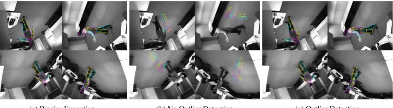
(a) Precise Execution (b) No Outlier Detection (c) Outlier Detection

Figure 2: Output Quality for Bodytrack

in a set of poses against an image. The computation is imple-mented as a set of Topaz tasks defined by the Topaz taskset construct. When it executes, the taskset generates a set of tasks, each of which executes three main components: the task compute block (which defines the approximate compu-tation of the task), transform block (which defines an out-put abstraction), and combine block (which integrates the computed result into the main computation).

compute block: The compute block defines the inputs (with section in), outputs (with section out) and compu-tation (following code block) associated with an approxi-mate task. In our example, the compute block computes the weight for a particular pose by invoking the CalcWeight function, which is a standard C function. The taskset ex-ecutes a compute task for each pose. In total, it exex-ecutes particles.size() tasks.

Each task takes as input two kinds of data: stable data, which has the same value for all tasks in the taskset (stable data is identified with the const keyword) and transient data (which may have different values for each task in the taskset). In our example each task has one transient input, tpart (which identifies the pose to score) and several stable inputs (that remain unchanged throughout the lifetime of the taskset): (1) tmodel, the model information (2) timg, the frame to process, (3) nCams, the number of cameras, and (4) nBits, the bit depth of the image. The task produces one result: tweight,

transform block: The transform construct defines the AOV, which captures the key features of the task result. Topaz performs outlier detection on this AOV when the task finishes execution. In this example we use the pose position from the task input (bp1,bp2,bp3) and pose weight from the task result (bweight) as the AOV.

combine block: When the task completes, its combine block executes to incorporate the results from the out pa-rameters into the main Topaz computation (provided the out-lier detector accepts the task). In our example, the combine block updates the mWeights global program variable.

2.2 Approximate Execution

The current Topaz implementation runs on an approximate computing platform with a precise processor and an approx-imate processor. The precise processor executes all non-taskset code and the transform and combine blocks of executed tasks. The approximate processor executes the compute bodies of the executed tasks. Since the taskset construct is executed approximately, the computed results may be inaccurate. In our example the task result, tweight (the computed pose weight), may be inaccurate. That is, the computed pose may be assigned an inappropriately high or low weight for the provided frame.

If integrated into the main computation, significantly in-accurate tasks can unacceptably corrupt the end-to-end re-sult that the program produces. In our example, the combine blocks write the computed weights into a persistent weight array mWeights. Bodytrack uses this weight array to select the highest weighted pose for each frame. If the computation incorporates an incorrect weight, it may select an incorrect pose as the best pose for the frame.

2.3 Outlier Detection

Topaz therefore deploys an outlier detector that is designed to detect tasks that produce unacceptably inaccurate re-sults. The outlier detector uses the user defined transform block to convert the task inputs and results into a numeri-cal vector, which we numeri-call the abstract output vector (AOV). This vector captures the key features of the task result. The transform block in our example defines a four dimensional AOV <bweight,bp1,bp2,bp3> comprised of the weight and pose position. We use this abstraction because we ex-pect poses in the same location to be scored similarly.

The outlier detector uses this numerical vector to perform outlier detection online (see Section 5.4 for more details). The outlier detector accepts correct AOVs and rejects AOVs that are outliers. In our example, the outlier detector rejects tasks that produce high weights for bad poses – poses that are positioned in parts of the frame without a person. Similarly, the outlier detector rejects tasks that produce low weights for good poses – poses near the person.

2.4 Precise Reexecution

When the outlier detector rejects a task, Topaz precisely re-executes the task on the precise processor to obtain the cor-rect task result, which it then integrates into the main com-putation. The numerical vector attained by transforming the task result is used to further update the outlier detector. To minimize any error-related skew, Topaz uses only correct re-sults attained via reexecution to train the outlier detector. In our example, the tasks that assign abnormally high weights to bad poses or low weights to good poses are rejected and reexecuted. After all task results have been integrated and the taskset has completed execution, the highest weight in the persistent weight array belongs to a pose close to the correct one. This technique maximizes the accuracy of the overall computation.

Figure 2a presents the correct pose for a particular video frame when the computation has no error. Figure 2b presents the selected pose for the same frame run on approximate hardware with no outlier detection. Note that the selected pose is unacceptably inaccurate and does not even loosely cover the figure. Figure 2c presents the selected pose for the same frame on the same approximate hardware with outlier detection. Observe that the chosen pose is visually indistin-guishable from the correct pose (Figure 2a). The numerical error for the computation with outlier detection is 0.161% (compared to 73.63% error for the computation with no out-lier detection). The outout-lier detector reexecutes 4.72% of the tasks, causing a 4.10% energy degradation when compared to the savings without detection (12.70% vs. 8.60%). With the Topaz overhead included, the reported energy savings are 7.69% (0.91% loss from Topaz overhead).

3.

The Topaz Language

We implement Topaz as an extension to C. Topaz adds a sin-gle statement, the taskset construct. When a taskset construct executes, it creates a set of approximate tasks that execute to produce results that are eventually combined back into the main computation. Figure 3 presents the general form of this construct.

taskset name(int i = l; i < u; i++) { compute in (d1 x1 = e1, ..., dn xn = en)

out (o1 y1, ..., oj yj) { <task body>

}

transform out(v1, ..., vk) { <output abstraction> }

combine { <combine body> } }

Figure 3: Topaz Taskset Construct

Each taskset construct creates an indexed set of tasks. Referring to Figure 3, the tasks are indexed by i, which ranges from l to u-1. Each task uses an in clause to specify

a set of in parameters x1 through xn, each declared as d1 through dn and initialized to expressions e1 through en. Topaz supports scalar declarations of the form double x, float x, and int x, as well as array declarations of the form double x[N], float x[N], and int x[N], where N is a compile-time constant. To specify that input parameters are stable and do not change throughout the lifetime of a taskset, we prepend the const identifier to the input type. Each task also uses an out clause to specify a set of out parameters y1 through ym, each declared as o1 through om. The task writes the results that it computes into these out parameters. As for in parameters, out parameters can be scalar or array variables.

Topaz imposes the requirement that the in and out pa-rameters are disjoint and distinct from the variables in the scope surrounding the taskset construct. Task bodies write all of their results into the out parameters and have no other externally visible side effects.

The transform body computes over the in parameters x1, ..., xn and out parameters o1, ..., oj to produce the numerical AOV v1, ..., vk. The outlier detector op-erates on the AOV.

The combine body integrates the task results into the main body of the computation. All of the task bodies for a given taskset are independent and can execute in parallel — only the combine bodies may have dependences.

4.

Abstract Output Vectors

A well-designed AOV is an efficient abstraction that exposes sufficient result quality information to the Topaz outlier de-tector. To work well, AOVs should be efficiently computable and produce a small set of numbers that make unacceptably inaccurate results readily apparent. Each AOV produces a floating point vector computed in the transform block. In general, larger dimension vectors and more complex trans-form blocks incur greater overhead.

4.1 Constructing an AOV

We consider two techniques for designing effective AOVs:

•Dimensionality Reduction: The transform block per-forms a reduction on the task results to reduce the di-mensionality of the AOV.

•Domain-Specific Normalization: The programmer uti-lizes domain knowledge to construct an AOV that re-moves the input correlation from the task results without explicitly including the inputs in the AOV.

Dimensionality reduction is an easy-to-apply generalized method that may be applied to any task. Normalization is typically closely tied to the application semantics. We use the blackscholes benchmark (see Section 6) to illustrate these two techniques. Blackscholes predicts the future price of a set of options, given the current prices and a set of option parameters (strike,volatility,time,type,rate). Each Topaz task computes prices for 64 options.

Figure 4: Effect of Performing Output Reduction

Dimensionality Reduction: We consider four blackscholes AOVs: (1) a one-dimensional AOV which sums all 64 pre-dicted prices to obtain a single element for outlier detection, (2) a two-dimensional AOV in which each element is the sum of 32 prices, (3) a four-dimensional AOV in which each element is the sum of 16 prices, and (4) an eight-dimensional AOV in which each element is the sum of eight prices.

Figure 4 presents the effect of dimensionality reduction on the error detection rate, option price error, and energy savings. As the dimensionality of the AOV increases, the error detection rate increases. In response, the computation becomes more accurate and the relative option price error decreases, but from an already very small base error (specif-ically, from 0.05% to 0.02%). Also in response, the energy savings drops. There are two contributing factors. First, in-creasing the dimensionality of the result increases the pre-cision of the outlier detector, which detects more errors and reexecutes more tasks as the dimensionality increases.1 Sec-ond, the increase in the dimensionality of the AOV increases the outlier detector overhead.

Contraindications for Dimensionality Reduction: Dimen-sionality reduction has almost no impact on the overall ac-curacy of blackscholes (in part because the correct option prices all have similar magnitudes). Combining results from radically different distributions may significantly degrade Topaz’s ability to perform error detection and noticeably im-pact result quality. For example, if one of the results tends to be large and the other result is small, the larger result may mask errors in the smaller result. In the barnes benchmark (see Section 6), the magnitude ranges of the acceleration and velocity task results are drastically different (-5 to 5 vs -150 to 150). Topaz detects 52.50% of the errors when the AOV combines like results and only 30.61% of the errors

1_{The target reexecution rate for these executions is zero. The outlier} detec-tor therefore does not contract its bounds in an attempt to obtain a higher reexecution rate.

(20% less) when the AOV combines unlike results. The cor-responding energy savings are 6.40% (when combining like results) and 7.91% (when combining unlike results). Dimensionality Reduction and Batching: The natural task granularity of some Topaz applications may be too small to profitably amortize the Topaz task management overhead. In such situations batching — combining multiple natural tasks into a single larger Topaz task — is one way to drive the Topaz task management overhead down to acceptable lev-els. Batched tasks typically produce multiple sets of results (one for each natural task in the batch). Batching can thefore often be productively combined with dimensionality re-duction for effective outlier detection, with like results from natural tasks combined into a single element for outlier de-tection. Blackscholes, for example, batches 64 natural tasks into a single Topaz task for a batching factor of 64. For this application (but not all Topaz applications, see Section 6), batching is essential for successfully amortizing the Topaz task management overhead.

Domain-Specific Normalization: We derive a domain-specific normalization for blackscholes using the no-arbitrage bound for European put-call options [11]. The no-arbitrage bound is a sane maximum and minimum option price, given the option parameters and price. The benchmark utilizes Eu-ropean put-call options. The original inequality is as follows:

if put: s · e−r ·t− p0≤ p ≤ p0 if call: p0− s · e−r·t≤ p ≤ s · e−r·t

Where s is the strike price, r is the rate, t is the time, p0is the input price and p is the result price. First, we normalize the lower bound to attain an expression for p.

if put: 0 ≤ p − s · e−r·t+ p0≤ 2 · p0− s · e−r·t if call: 0 ≤ p − p0+ s · e−r · t≤ 2 · s · e−r·t_{− p0}

We then normalize the expression against the upper bound by dividing out the upper bound.

if put: 0 ≤ (p − s · e−r·t+ p0) · (2 · p0− s · e−r· t)−1 ≤ 1 if call: 0 ≤ (p − p0+ s · e−r·t) · (2 · s · e−r·t− p0)−1 _{≤ 1}

Note that the type variable determines whether the opera-tion is a put or call operaopera-tion. The above expression pro-vides a normalized representation of p, where it is unlikely that p falls outside of the range [0, 1].

With the no-arbitrage normalization applied, the Topaz outlier detector catches 8% more errors (reexecuting 0.02% more tasks) and loses 7% energy savings in comparison with an AOV that simply uses the computed option price. We attribute the lost energy savings to the more complex AOV computation as reflected in the formulas above. This example illustrates how an effective AOV must balance a number of factors including reexecution rate, accuracy, and AOV compute time.

4.2 AOVs and Quality Metrics

Note that although we use result quality metrics to evaluate the quality of the AOV, we decouple the AOV definition from the quality metric of the application when constructing the AOV. We intentionally decouple the two phenomena because quality metrics introduce the following complexities:

•_{Expensive to Compute: Some quality metrics can be}

more expensive to specify and compute than AOVs. For example, a quality metric may involve a comparison with a reference result which can be expensive to compute.

•Indirect Measure of Detector Performance: Quality metrics often have an indirect relationship to the efficacy of the outlier detector since the computed taskset result flows through the rest of the program, which may further amplify or dampen any taskset inaccuracy.

In contrast, AOVs are typically easier to specify and com-pute — they are specified at the task level, work only with task inputs and results, and are designed only to enable the detection of unacceptably inaccurate results, rather than provide a full quantitative measure of quality. They there-fore typically involve less specification overhead than a full-blown quality metric and are more closely tied to the perfor-mance of the outlier detector.

On Synthesizing AOVs: It is possible to automatically syn-thesize an AOV given an application, representative input(s), and target energy savings and result quality goals. The syn-thesis procedure would empirically explore the space of re-ductions applied to the task results to find an AOV that satis-fied the target energy savings and result quality goals for the application running on the representative input(s).

4.3 Application Classes and AOVs

There are some classes of applications for which designing an AOV may be challenging or difficult. For these applica-tions, the programmer may have to choose between carefully designing a domain-specific AOV or using an AOV which is a suboptimal proxy for the quality of the task results. We next discuss two potentially problematic classes of applica-tions.

Applications with Irreducible, Complex Task Outputs: Applications which contain large or complex irreducible task results may complicate the design of efficient AOVs. For such applications AOVs that work with all or most of the result components may be unacceptably inefficient. Compu-tations with tasks that produce large segments of unstruc-tured data (such as image data produced by graphics appli-cations) may exhibit these characteristics.

Uncheckable Applications: In some applications an appro-priate result distribution may be difficult to learn or infea-sible to compute without imposing unacceptable overhead. Tasks with complex result constraints or, conversely, com-pletely unpredictable results, may exhibit these characteris-tics.

5.

Topaz Implementation

The Topaz implementation is designed to run on an approx-imate computing platform with one precise processor and one approximate processor. The precise processor executes the main Topaz computation, which maps the Topaz tasks onto the approximate processors for execution. The Topaz implementation contains four components: (1) a front end that translates the taskset construct into C-level Topaz API calls, (2) a message-passing layer for dispatching tasks and collecting results, (3) an outlier detector that prevents un-acceptably inaccurate task results from corrupting the final result, and (4) a fault handler for detecting failed tasks.

5.1 Topaz Compiler

As is standard in implementations of task-based languages that are designed to run on distributed computing plat-forms [34], the Topaz implementation contains a compiler that translates the Topaz taskset construct into API calls to the Topaz runtime. The Topaz front-end is written in OCaml. The front-end generates task dispatch calls that pass in the input parameters defined by the in construct, the task index, and the identifier of the task to execute. The front end gener-ates the code required to send the task results (the task’s out parameters) to the precise processor running the main com-putation. The front end also extracts the different pieces of the taskset (the task body, combine block, and transform block) into invocable functions.

The Topaz compiler generates code for the Topaz data marshalling API, which coordinates the movement of tasks and results between the precise and approximate processors. 5.2 Topaz Runtime

The Topaz implementation works with a distributed model of computation with separate processes running on the pre-cise and approximate processors. Topaz includes a standard task management component that coordinates the transfer of tasks and data between the precise and approximate pro-cessors. The current Topaz implementation uses MPI [12] as the communication substrate that enables these separate processes to interact. It is also obviously possible to im-plement Topaz on shared memory machines using standard techniques [34].

To amortize the communication overhead, Topaz divides task data into two types: stable data and transient data. Stable data does not vary over the lifetime of the taskset. It is therefore sent over with the first task, reused in place for subsequent tasks, and refreshed (sent over again) if the Topaz implementation detects three consecutive incorrect tasks. Transient data may vary across tasks and is sent over with every task.

To execute a taskset, Topaz first sends the stable data to the approximate processor. It then executes the tasks in the taskset as follows:

•_{Task Creation: The precise processor sends the task,}

in-cluding the transient data, to the approximate processor.

•Task Execution: The approximate processor receives the task and executes the task’s compute block to obtain the task results.

•Task Response: The approximate processor sends a mes-sage containing the task results back to the precise pro-cessor running the Topaz main computation.

•Outlier Detection: The precise processor executes the task’s transform block to compute the abstract output vector (AOV) for the task. It then runs the outlier detector on the AOV. If the detector accepts the result, Topaz runs the task’s combine body to integrate the result into the main computation. If the detector rejects the result:

Task Reexecution: It reexecutes the task on the pre-cise processor to obtain the correct result. It then runs the combine block to integrate this correct result into the Topaz main computation.

Outlier Detector Update: It uses the correct result to update the outlier detector (see Section 5.4).

Stable Data Resend: If the task is the third consec-utive incorrect task, Topaz resends the stable data to the approximate processor. This feature was imple-mented to counteract the degradation of stable data in approximate memories (the values of stable data may degrade/change over time as the memory cells lose capacitance). Because the degradation of stable mem-ory is only one of several sources of error, and to avoid unnecessary communication overhead, the Topaz im-plementation resends the stable data only after it ob-serves three consecutive incorrect tasks.

5.3 Failed Task Detection

Topaz also handles cases where the task fails to complete execution on the approximate processor. In the event a task fails, the approximate processor notifies the main proces-sor. Topaz reexecutes the task on the main processor and refreshes the stable data on the approximate machine. It is straightforward to extend Topaz to handle infinite loops by modelling the task runtimes and reexecuting tasks that take unacceptably long. If the precise reexecution also contains an infinite loop, it is possible to apply the same model and discard the task [5, 17, 32].

5.4 Outlier Detection

For each taskset, Topaz builds an outlier detector designed to separate incorrect AOVs from correct AOVs. Topaz per-forms outlier detection when a task is finished but prior to result integration. It first runs the transform block to obtain the AOV for the task. The outlier detector then processes the AOV to either accept or reject the task. If it rejects the AOV, Topaz reexecutes the task on the precise processor to obtain

correct results and re-sends the stable task data. The AOV of the correct result is used to train the outlier detector. We use the following notation:

•_{t: We use t to denote a task vector, which is comprised of}

task data and the task results. We denote the task vector from the precise machine as tp.

•aov(t), ||aov(t)|| = d: The function notation for apply-ing the transform block, which transforms the task vector into an AOV. The resulting AOV has dimensionality d.

•reexec(t): Reexecute the task using inputs defined by the task vector t on the reliable machine, to obtain a new (correct) task vector.

•w, w⊥, w>, wµ, wn: We denote outlier detector re-gions with w. Rere-gions are d dimensional hypercubes, where we define the bottom corner, top corner, center of mass and number of test points in a region w using w⊥, w>, wµ, wnrespectively.

•_{W = {w}: We define W as the set of regions used by}

the outlier detector. We use ||W || to denote the number of regions the detector is using.

•l: The user-specified maximum number of regions the outlier detector may use. This bound limits the complex-ity of the outlier detector.

Testing: The outlier detector maintains a set of regions, where each region models a hypercube that encapsulates a part of the distribution of the correct AOVs. If the AOV that is being tested falls into any of these regions, the task result is considered a valid result and accepted; otherwise, the task result is rejected and the task is reexecuted. Consider t, a task vector produced by an approximate worker machine. Figure 5 presents the algorithm for determining whether to accept or reject the task:

bool is_acceptable(t): v = aov(t)

for w ∈ W :

bool enc = true for 0 ≤ i < d:

enc = enc && (w⊥(i) ≤ v(i) ≤ w>(i)) if enc:

wn += 1 return true; end

return false

Figure 5: Task Outlier Detection Algorithm Training: Figure 8 presents the algorithm for training the outlier detector. The outlier detector runs this algorithm only after it rejects a task, then reruns the task on the precise processor to obtain the correct task vector tp. If the correct AOV is already included in one of the regions of the outlier detector, the outlier detector updates the region’s center of mass. Otherwise, it creates a new region containing just the

double score(w,y): overlap = 1 for 0 ≤ i < d: if w⊥(i) > y⊥(i): ov = w>(i) − y⊥(i) else: ov = y>(i) − w⊥(i) if ov < 0: ov = 0 overlap = overlap*ov if overlap > 0: return overlap center_distance = 0 for 0 ≤ i < d:

center_distance += (wµ(i) − yµ(i))2 return -center_distance

Figure 6: Region Proximity Scoring Algorithm

region merge(w,y): z = new region() zn = wn + yn for 0 ≤ i < d: z>(i) = max(w>(i),y>(i)) z⊥(i) = min(w⊥(i),y⊥(i)) zµ(i) = _z1

n (wµ(i) · wn + yµ(i) · yn) return z

Figure 7: Region Merge Algorithm

AOV and adds it to the set of regions. If the outlier detector contains more than the maximum number of regions, it uses the scoring algorithm to find the two most similar regions and merges them (using the merge algorithm).

•_{Scoring: If the regions overlap, the score is the product of}

the magnitude of the overlapping region along each axis. The regions must overlap across all axes in order for them to be overlapping. If the regions are non-overlapping, the score is the negative distance between centers (to penalize distant, non-overlapping regions). The higher the score, the more similar the regions.

•Merging: The merged region is an n-dimensional hyper-cube enclosing both regions with a center of mass that is the weighted average of the two regions’ centers of mass. 5.5 Outlier Detector with Contraction

The outlier detector has an extension which contracts the region’s bounds when the reexecution rate falls below the user-defined target reexecution rate. Contracting the region’s bounds increases the reexecution rate because the outlier

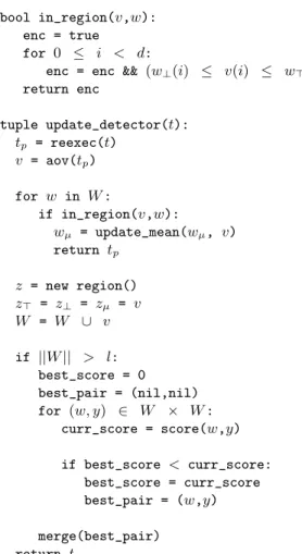
bool in_region(v,w): enc = true

for 0 ≤ i < d:

enc = enc && (w⊥(i) ≤ v(i) ≤ w>(i)) return enc tuple update_detector(t): tp = reexec(t) v = aov(tp) for w in W : if in_region(v,w): wµ = update_mean(wµ, v) return tp z = new region() z> = z⊥ = zµ = v W = W ∪ v if ||W || > l: best_score = 0 best_pair = (nil,nil) for (w, y) ∈ W × W : curr_score = score(w,y) if best_score < curr_score: best_score = curr_score best_pair = (w,y) merge(best_pair) return tp

Figure 8: Outlier Detector Training Algorithm

detector rejects tasks whose AOVs would have previously fallen on the fringe of the hypercube defined by the region. This mechanism allows the outlier detector to disclude fringe values from the region and adapt to changing AOV distribu-tions.

We augment the outlier detector so that each region also contains a Proportional-Integral-Derivative (PID) control system, which controls the region contraction. We define the notation for the control system as follows:

•γ = γr, γc, γR, γ∂: The Proportional-Integral-Derivative (PID) control system γ comprised of the running reexe-cution rate (γr) and the current (γc), integral (γR), and discrete derivative (γ∂) of the difference between the tar-get and running reexecution rate.

•Kc, KR, K_∂: Weights associated with the PID control system.

•ctrl(w): The control system associated with region w.

•g: The user defined target reexecution rate. This bound limits the reexecution overhead and controls the contrac-tion of the regions.

•_{update control(γ,u): given u, where u is 0 if the AOV}

was accepted or 1 if the AOV was rejected, update the control system γ.

•get contract(γ): get the region contraction factor for the given control system γ.

•update running rate(γr, u): Given the running reexe-cution rate γrand u (as defined above), update and return the running reexecution rate.

•update running integral(γR, γc): Given the current in-tegral of the difference between the target and running reexecution rate, update and return the integral.

We next discuss two algorithms: (1) updating the control system and the (2) contracting the region bounds.

Control System Get: Figure 9 presents the algorithm for getting the contraction rate. To compute the contraction rate, we use the PID control formula, a standard technique in con-trol systems. This formula uses the integral, derivative and current reexecution rate to compute the contraction rate.

double get_contract(γ):

F = Kc· γc+ KR · γR + K∂· γ∂ return F

Figure 9: Contraction Rate Computation

Control System Update: Figure 10 presents the algorithm for updating the control system. It first updates the running reexecution rate to include the outcome of the testing the last task. It then updates the derivative, running integral, and present difference between the running reexecution rate and target rate and returns the new control system.

object update_control(g,γ,u): γr = update_running_rate(γr,u) i = γr- g γ∂ = i − γc γc = i γR = update_running_integral(γR,γc) return γ

Figure 10: Control System Update

Region Contract: Given the target rate, the approximate AOV, whether the AOV was accepted, and the region the AOV belongs to, the algorithm in Figure 11 adjusts the re-gion. The algorithm operates as follows.

It first updates the region’s rejection rate based on whether the last point was accepted or rejected. It then queries the control system to obtain F, the factor by which to contract the region. It clamps the contracting factor to (0.5, 1) so that region doesn’t shrink by more than half its size. It finally scales the region relative to its center of mass.

function contract_region(g,w,u) γ = ctrl(w) γ = update_control(g, γ, u) contraction_factor = get_contract(γ) F = min(max(contraction_factor,1),0.5) for 0 ≤ i < d

w>(i) = wµ(i) + F · (w>(i) − wµ(i)) w⊥(i) = wµ(i) − F · (wµ(i) − w⊥(i))

Figure 11: Region Contract

5.6 Mathematical Model

We next present a simple mathematical model that may be used to predict energy savings and outlier detector efficacy across the space of reexecution rates, taskset sizes, and ab-straction configurations. To simplify the presentation, we as-sume the application executes one taskset and that all tasks in that taskset execute the same number of instructions. It is straightforward to generalize the model to include multiple tasksets and tasks with varying numbers of instructions:

•n: The number of tasks in the taskset.

•_{r: The number of reexecuted tasks. This may be}

approx-imated from a reexecution rate v using: r = n · v

•_{c: The number of stable data transfers.}

•p, q, o: The size of transient data (p), stable data (q), and task results (o), in bytes.

•d: The dimensionality of the AOV emitted by the trans-form block.

•l: The maximum number of regions used by the outlier detector.

•T , V , M : The number of instructions in a task (T ), AOV transformation (V ), and the total number of non-taskset instructions (M ).

We also consider the following Topaz parameters:

•ıp, ıa: Topaz initialization overhead for the precise (ıp) and approximate (ıa) processors.

•_{σ,ρ: Per-task Topaz instruction overhead for}

communi-cating data, per byte, for sending (σ) and receiving (ρ) data.

•τm, τw: Per-task Topaz instruction overhead not associ-ated with data communication, precise (τp) and approxi-mate (τa) processors.

•α: Per-task AOV computation overhead.

•δt, δr: Per-task, per detector region, and per AOV dimen-sion detector testing (δt) and training (δr) overhead. We also consider ∆, the energy consumption of the approxi-mate processor relative to the precise processor. We

approx-imate the Topaz overhead on the precise (Op) and approxi-mate (Oa) processors as follows:

Op= ıp+ σ · c · q + σ · n · p + ρ · n · o + τp· n Oa= ıa+ ρ · c · q + γ · n · p + σ · n · o + τa· n Essentially, we sum up the initialization overhead, commu-nication overheads and per-task runtime overheads to deter-mine the Topaz overhead.

Next we compute the detection overhead:

D = δr· r · d · l + δt· n · d · l + V · (n + r) Finally, we model the energy savings as follows:

S = 1 −T · r + M + D + Op+ ∆ · [T · n + Oa] M + T · n

We use this model to approximate the energy consumption, given a particular set of parameters.

Software and Hardware Interdependences: The above model does not attempt to derive task error rates as a function of hardware error rates because the hardware error character-istics and software charactercharacter-istics are often interdependent:

•_{Stateful Errors: Some classes of errors, such as memory}

errors, are stateful and may persist across tasks.

•_{Hardware-Dependent Errors: Some classes of errors,}

such as cache and memory errors, depend on which data is loaded into cache and memory (as well as the values of that data), which depends on the behavior of the applica-tion.

•Time-Dependent Errors: Some classes of errors, such as memory decay errors, have error rates that are func-tions of time (time since last refresh). Since data is re-freshed when it is written, these errors can also depend on the behavior of the application.

6.

Experimental Results

We present experimental results for Topaz implementations of our set of five benchmark computations:

•_{blackscholes: A financial analysis application from the}

Parsec benchmark suite that solves a partial differential equation to compute the price of a portfolio of European options [2].

•water: A computation from the SPLASH2 benchmark suite that simulates liquid water [33, 48].

•barnes: A computation from the SPLASH2 benchmark suite that simulates a system of N interacting bodies (such as molecules, stars, or galaxies) [48]. At each step of the simulation, the computation determines the forces acting on each body, then uses these forces to update the positions, velocities, and accelerations of the bodies [1].

•_{bodytrack: A computation from the Parsec benchmark}

suite that tracks the pose of the subject, given a series of frames [2].

•streamcluster: A computation from the Parsec bench-mark suite that performs hierarchical k-means clustering [2].

We provide an artifact containing detailed instructions for installing Topaz and replicating the experiments, as well as a Virtualbox virtual machine image and EC2 AMI image containing the Topaz environment [37].

6.1 Experimental Setup

We perform our experiments on a simulated computational platform with one precise processor and one approximate processor. There is one process per processor; the processes communicate using the MPI message passing interface [12]. Caches and Memories: The computational platform con-tains a memory hierarchy with a mix of reliable and unreli-able components.

Caches:The precise processor has a precise L1 instruction and data cache, while the approximate processor has a pre-cise L1 instruction cache and mixed prepre-cise-approximate L1 data cache. Each processor has a larger, mixed precise-approximate L2 cache with the same cache line size as the L1 cache. The mixed precise-approximate caches are dual voltage caches where cache lines may be flagged to use re-duced voltage [9]. In our evaluation all critical data is stored in high voltage cache lines, while task data is stored in low voltage cache lines. The fault characteristics for these ap-proximate caches are modelled as probabilistic write cor-ruptions and read corcor-ruptions [35]. Table 1 presents the fault and energy characteristics for approximate caches. In our cache hierarchy, we model 16K,4 Way,16 byte/line L1i and L1d caches and a 64K,8 Way,16 byte/line L2 cache. Main Memory:Main memory is divided into precise, high refresh DIMMs and no refresh DIMMs. Prior work mod-els DRAM faults as random corruptions that occur in non-refreshed cells over time. For our evaluation, we construct the per-millisecond bit flip probability model by modelling the regression of Flikker’s DRAM error rates and use the energy consumption associated with DRAM refresh to com-pute energy savings [22]. We also consider a more sophis-ticated fault model where the per-millisecond error rate per row fluctuates based on DIMM activity [21]. Table 1 presents the fault and energy characteristics for approximate DRAMs. We store all stable and transient data associated with task execution in the no-refresh DRAMs. We assume 40% percent of the memory banks are approximate. Bit Pattern Dependence:Recent research has found a signif-icant fraction of DRAM errors are dependent on the values of the data stored in DRAM [21]. In a DIMM, bitline-bitline and bitline-wordline coupling effects impact the cell leak-age. That is, neighboring cells may influence the value read

Property Error Probability Sram read upset probability† 10−7.4/ read Sram write upset probability† 10−4.94_{/ write}

Supply Power Saved† 80%

Fraction energy consumption† 0.2996%

L1 Cache Size 16K

L1 Cache Associativity 4 ways L1 Cache Line Size 16 bytes

L2 Cache Size 64K

L2 Cache Associativity 4 ways L2 Cache Line Size 16 bytes Dram per-word error

probability over time (cell/ms)†† 3 · 10−7_{· t}2.6908

Dram Energy Saved†† 33%

Fraction energy consumption† 0.7009 Fraction DRAM no-refresh 0.40

Table 1: Hardware Model Parameters. †: from Enerj Paper ( [35]). ††: from Flikkr Paper [22].

from the target cell[14]. The effect can be described as fol-lows: if the target cell contains a logic 1 and the adjacent cell also contains a logic 1, the target cell is considered stressed and may be read as a 0. If the target cell contains a logic 0 and the adjacent cell contains a logic 0, the target cell is con-sidered stressed and may be read as a 1.

Hardware Models:In the basic hardware model, we use the fixed DRAM error rate seen in previous work [35]. In our ddep hardware model, we model the dependence between the retention time of data in a row and the data stored in the DIMM as described above.

Hardware Emulator: To simulate the approximate hard-ware we implemented an approximate hardhard-ware emulator using the Pin [23] binary instrumentor. We based this emula-tor on on iAct, Intel’s approximate hardware tool [27]. Our tool instruments memory and stack reads to access simulated versions of the caches and main memory described above, using the fault parameters from Table 1. We have included a specialized API for setting the hardware model and en-abling/disabling fault injection. We track various statistics, such as the cache hit and miss rates and the average fraction of unreliable lines in cache, to populate the energy model.

We simulate the time-dependence of DRAM error proba-bility by increasing the probaproba-bility of a DRAM error in ac-cordance with the model every 104instructions, or 0.01 mil-liseconds (for a 2GHZ machine). For the ddep model, we simulate the data-dependence of the DRAM error probabil-ity by modelling a simplified version of bitline coupling. We attach a multiplier (up to 2x) to the nominal error rate in Ta-ble 1 wi ∈ {1.0, 2.0} depending on the parity of the neigh-bors compared to the bit being read. This model assumes contiguous regions of memory are spatially co-located in the DIMMs.

Hardware Energy Model: We next present our hardware energy savings model. We break up energy consumption into the SRAM energy consumption and DRAM energy consumption.

Cache Energy Savings:For each cache C, we consider the following parameters: the average fraction of approximate lines in the cache βc, the size of the cache Sc, the relative energy consumption (1-savings) for low power cache lines ψlow, and the energy consumption for high power cache lines ψhigh (1) (see Table 1). We consider the following caches: C = {L1I, L1D, L2}. The energy consumption of the approximate cache hierarchy relative to the precise cache hierarchy is as follows: ∆C= P c∈Cβc· Sc· ψlow+ (1 − αc) · Sc· ψhigh P c∈CSc· ψhigh

Main Memory Energy Consumption:We assume a constant fraction of memory, βm, is no-refresh. We assume all banks are in use. Given the energy consumption for no refresh memories ψnoref and refresh memories ψref (see Table 1), we compute the approximate DRAM consumption relative to the fully precise energy consumption as follows:

∆M = βm· ψnoref+ (1 − βm) · ψref ψref

Cache + Memory Energy Consumption:We parameterize the formula with fd, the fraction of system energy con-sumption from memories and fc, the fraction of system en-ergy consumption for caches. See Table 1 for parameters. We compute the energy consumption of the approximate cache+memory system relative to the precise system as fol-lows:

∆ = ∆Mfd+ ∆Cfc 6.2 Benchmark Executions

We present experimental results that characterize the accu-racy and energy consumption of Topaz benchmarks under a variety of conditions:

•Precise: We execute the entire computation, Topaz tasks included, on the precise processor. This execution pro-vides the precise, fully accurate results that we use to evaluate the accuracy of the other executions.

•_{No Topaz: We attempt to execute the full computation,}

main Topaz computation included, on the approximate processor. For all the benchmarks, this computation ter-minates with a segmentation violation.

•_{No Outlier Detection: We execute the Topaz main}

com-putation on the precise processor and the Topaz tasks on the approximate processor with no outlier detection. If a task crashes and does not return a result, the Topaz imple-mentation reexecutes the task on the precise processor. Stable data is only resent when three consecutive tasks crash. We integrate all of the results from approximate tasks that do not crash into the main computation.

•Outlier Detection: We execute the Topaz main compu-tation on the precise processor and the Topaz tasks on the approximate processor with outlier detection and reexe-cution as described in Section 5.

No Outlier Outlier Benchmark Model Detector Detector

barnes basic inf 0.158229%

blackscholes basic inf 0.135584%

bodytrack basic 73.6327% 0.161024% streamcluster basic 0.6219 0.6344

water basic nan 0.000469%

barnes ddep inf 0.075927%

blackscholes ddep inf 0.025791%

bodytrack ddep 73.6327% 0.317984% streamcluster ddep 0.6321 0.6344

water ddep nan 0.000383%

Table 2: End-to-End Output Quality

6.3 Benchmark AOVs

We use the following AOVs:

•_{barnes: Each task is the force calculation computation}

for a particular body. The tasks are batched such that each task computes the velocity and acceleration of two bodies. The AOV is the amplitude of the velocity and acceleration vectors and the scalar result phi.

•bodytrack: Each task is the weight calculation of a par-ticular pose in a given frame on the approximate machine. The AOV is the position vector and weight.

•streamcluster: Each task is a subclustering operation in the bi-level clustering scheme. The AOV is the gain of opening/closing the chosen centers and the sum of weights assigned to the points in the subclustering op-eration.

•_{water: Two computations execute on the approximate}

machine: (1) the intermolecular force calculation, which determines the motion of the water molecules (interf) (2) the potential energy estimation, which determines the potential energy of each molecule (poteng). The tasks are batched such that each task computes sixty four forces/energies. The AOVs are as follows:

interf: The AOV is the cumulative force exerted on the H,O,H atoms in the x,y and z directions and the scalar result incr.

poteng: The AOV is the sum of the magnitude of potential energy in the x,y and z directions.

•blackscholes: Each task is a price prediction on the ap-proximate machine. These tasks are batched such that each task computes 64 prices. The single dimensional AOV is the sum of the 64 computed prices.

6.4 End-to-End Output Quality

Table 2 presents the end-to-end output quality metrics for the (1) No Outlier Detection and (2) Outlier Detection cases. With one exception (streamcluster), executing the bench-marks with no outlier detection produces unacceptably in-accurate results. With outlier detection, the output quality is always acceptable and typically very small.

barnes: The output quality metric is the percent positional error (PPE) of each body. With outlier detection, the PPE

(a) Correct (b) No Detection (c) Outlier Detection

(d) Correct (e) No Detection (f) Detection

(g) Correct (h) No Detection (i) Detection

Figure 12: Visual Representation of Output Quality. (a-c) Barnes. (d-f) Water. (g-i) Streamcluster.

between the precise and approximate executions is a fraction of a percent and visually indistinguishable in the output. See Figures 12a and 12c, which plot the positions of the bodies at the end of the simulation. Figure 12c overlays the posi-tions of the bodies from the precise execution (in red) and the approximate execution with outlier detection (in black). Figure 12b plots the output from the approximate compu-tation without outlier detection (almost all of the bodies lie outside the plotted range).

blackscholes: The quality metric is the cumulative error of the predicted stock prices with respect to the total portfolio value. Without outlier detection, the percent portfolio error is many times more than the value of the portfolio. With outlier detection, the portfolio error is a fraction of a percent of the value of the portfolio.

bodytrack: The quality metric is the weighted percent error in the selected pose for each frame. In both the basic and ddep hardware models, we observed wildly incorrect pose choices. With outlier detection, the selected poses are visu-ally good matches for the body. Figures 2c and 2a present a visual comparison.

streamcluster: The quality metric is the weighted silhouette score, which is a measure of cluster quality - the closer to one, the better the clusters. The silhouette score with fully precise execution is 0.557. Figures 12g-12i) plot the input data (black dots) and the cluster centers (red dots). The pre-cise (Figure 12g) cluster centers are visually similar to the cluster centers produced by the approximate machine with no outlier detection (Figure 12h) and with outlier detection (Figure 12i). We attribute this result the robustness of the computation, which is inherently resilient to outliers.

More-Hardware Correct Correct Error Error Rejection Errors Benchmark Model Accepted (%) Rejected (%) Accepted (%) Rejected (%) Accuracy (%) Detected (%)

barnes basic 94.48% 0.19% 2.94% 2.38% 92.58% 44.74% bodytrack basic 87.58% 0.16% 7.67% 4.58% 96.62% 37.39% water-interf basic 95.30% 0.32% 1.71% 2.67% 89.37% 60.96% water-poteng basic 99.51% 0.26% 0.02% 0.20% 43.59% 89.47% blackscholes basic 98.57% 0.04% 1.06% 0.33% 90.00% 24.06% streamcluster basic 98.34% 0.14% 0.37% 1.15% 89.15% 75.66% barnes ddep 94.22% 0.20% 3.11% 2.47% 92.59% 44.26% bodytrack ddep 77.34% 0.15% 16.04% 6.46% 97.67% 28.71% water-interf ddep 95.44% 0.33% 1.62% 2.61% 88.81% 61.71% water-poteng ddep 99.49% 0.26% 0.04% 0.21% 44.54% 85.48% blackscholes ddep 98.70% 0.04% 0.94% 0.33% 89.80% 25.88% streamcluster ddep 62.24% 0.11% 36.68% 0.98% 89.90% 2.59%

Table 3: Overall Outlier Detector Effectiveness

over, the precise machine performs the top-level clustering operation, since errors in the top level clustering operation would have a disproportionate effect on the output. These two properties make introducing non-existent clusters and eliminating well-represented clusters unlikely — for this to occur, the approximate hardware would have to systemati-cally produce errors that result in selecting (or excluding) particular subsets of points.

water: The output quality metric is the percent positional er-ror (PPE) of each molecule. With outlier detection, the PPE between the precise and approximate executions is a frac-tion of a percent. The approximate molecule posifrac-tions with outlier detection (Figure 12f) are visually indistinguishable from the precise molecule positions (Figure 12d). Figures 12d-12f plot the positions from precise execution (in red), and the approximate execution (in black). Figure 12e plots the output from the approximate execution without outlier detection (almost all of the molecules lie outside the plotted range).

6.5 Outlier Detector Effectiveness

Table 3 presents data that characterizes the overall effective-ness of the outlier detector. The third through sixth columns present a breakdown of all of the tasks into correct tasks that were accepted (third column) or rejected (fourth col-umn) by the outlier detector and incorrect tasks that were accepted (fifth column) or rejected (sixth column). The sev-enth column (Rejection Accuracy) presents the percentage of rejected tasks that contain errors. The eighth column (Er-rors Detected) presents the percentage of tasks with er(Er-rors that were rejected.

These numbers indicate that, in general, (1) the majority of the tasks are correct and accepted by the outlier detector (column three, Correct Accepted) and (2) a large percentage of the rejected tasks contain errors (with the exception of water-poteng) (column seven, Rejection Accuracy). Even though the outlier detector rejects at most a few percent of the tasks, the data in Table 2 show that if the outputs from these few percent of the tasks are incorporated into the main computation, they produce unacceptably inaccurate results.

Detect & Full Benchmarks Model Baseline Reexecute Topaz

barnes basic 17.47% 14.77% 13.02% blackscholes basic 16.20% 14.62% 9.94% bodytrack basic 12.70% 8.60% 7.69% streamcluster basic 16.87% 15.62% 11.03% water basic 18.41% 15.12% 12.43% barnes ddep 17.47% 14.76% 13.02% blackscholes ddep 16.02% 14.41% 9.70% bodytrack ddep 12.88% 6.51% 5.02% streamcluster ddep 16.89% 15.58% 11.03% water ddep 18.41% 15.37% 12.82%

Table 4: Energy Savings, basic and ddep Hardware Models

Across applications, many of the incorrect tasks produce results that are embedded within the range of correct out-puts. The outlier detector therefore accepts these tasks (com-pare column five, Error Accepted, and column six, Error Re-jected). Since the errors for these tasks are small, they are acceptably inaccurate and have (very) acceptable impact on the overall end-to-end output quality. The outlier detector is effective at detecting the (in most applications relatively few) unacceptably inaccurate tasks that would cause the applica-tion to produce unacceptable end-to-end quality.

6.6 Energy Savings

Table 4 presents the energy savings for our benchmark appli-cations. We break the computation into the following com-ponents: instruction count of the main computation on the precise processor M , instruction count of tasks executing on the approximate processor A, instruction count of outlier detection routine and task reexecution on the precise pro-cessor R, and the overhead from the Topaz implementation and marshalling/unmarshalling task data L. For the simple model presented in Section 5.6 (a Topaz program with a single taskset with n tasks, each of which executes T in-structions, r reexecuted tasks, D detector overhead, and Op and OaTopaz overhead on the precise and approximate pro-cessors, respectively), A = T · n, R = T · r + D, and L = Op+ ∆ · Oa. For each benchmark, Table 4 presents the following three energy savings metrics:

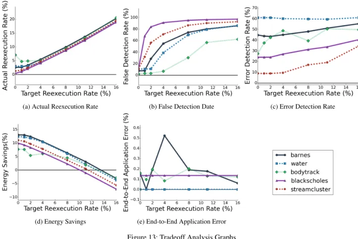
(a) Actual Reexecution Rate (b) False Detection Date (c) Error Detection Rate

(d) Energy Savings (e) End-to-End Application Error

Figure 13: Tradeoff Analysis Graphs

Target Reexecution Rate 0.00% 1.00% 2.00% 4.00% 8.00% 11.00% 16.00% Silhouette Score 0.634 0.635 0.629 0.635 0.634 -1.000 0.635

Table 5: Output Quality vs Reexecution Rate for Streamcluster

Baseline: The baseline energy savings available from exe-cuting tasks on the approximate processor:

1 − M + ∆ · A M + A

Detect & Reexecute: The energy savings including outlier detection and task reexecution on the precise processor:

1 − M + ∆ · A + R M + A

Full Topaz: The energy savings, with outlier detection and task reexecution, accounting for the Topaz overhead, includ-ing the overhead devoted to coordinatinclud-ing the distribution of the computation across the precise and approximate proces-sors:

1 − M + ∆ · A + R + L M + A

Each row presents the Baseline, Detect & Reexecute, and Full Topaz savings metrics for the application specified in the first column (Benchmark). The maximum attainable

savings is 19.185%, which is attained when all of the lines in the approximate caches are approximate lines, there is no overhead, and all of the computation executes on the approximate processor. The numbers in the table are for a target reexecution rate of zero — the outlier detector bounds grow to include the correct task results and never contract. At higher target reexecution rates, the outlier detector control algorithm contracts the bounds, detects more incorrect tasks, and the energy consumption and number of reexecuted tasks grows (see Figures 13d and 13c).

6.7 Crossover Analysis

We evaluate the effect of different target reexecution rates on percent errors detected and output quality. Figures 13a-13e present the results for each benchmark (we report results for the basic hardware model).

For all applications, the Topaz control system effectively matches the actual task reexecution rate with the target reex-ecution rate (Figure 13a). For some benchmarks, the control system fails to meet the target rate for low reexecution rates

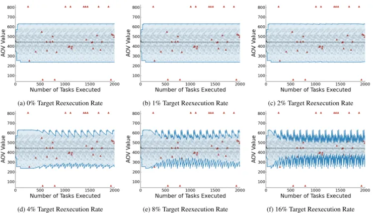
(a) 0% Target Reexecution Rate (b) 1% Target Reexecution Rate (c) 2% Target Reexecution Rate

(d) 4% Target Reexecution Rate (e) 8% Target Reexecution Rate (f) 16% Target Reexecution Rate

Figure 14: Time Series Visual Representation of Outlier Detector Behavior. Gray circles indicate correct tasks, red triangles indicate tasks with errors, the blue lines indicate the outlier detector bounds, and the black dashed line is the center of mass of the tasks that the outlier detector accepts. The shaded region is the region the outlier detector accepts.

because too many AOVs fall outside the envelope defined by previously seen AOVs to attain the reexecution rate.

As the target reexecution rate increases, the percentage of detected errors (and reexecuted tasks) increases (Fig-ure 13c). Increasing the target reexecution rate also dras-tically increases the percent of reexecuted tasks that have no errors (Figure 13b) — increasing the reexecution rate causes the detector to contract its regions, cutting into the periphery of the AOV distribution. Although there are some errors at the periphery, most of the AOVs are correct, which is why the false detection rate increases more quickly than the error detection rate.

The task reexecutions decrease the energy savings (Fig-ure 13d), with the crossover point from energy savings to increased energy consumption occurring between a target re-execution rate of 10% (blackscholes) to 14% (barnes,water). The crossover point occurs when the application curve in-tersects the 0% energy savings axis (black horizontal line, Figure 13d).

Figure 13e presents the end-to-end application error for all applications except streamcluster (all of these application error metrics are computed relative to the output from the precise execution). Table 5 separately presents the Silhouette end-to-end quality metric for streamcluster. The end-to-end output quality (Figure 13e and Table 5) is largely unaffected

by the target reexecution rate. We attribute this phenomenon to (1) the outlier detector’s ability to effectively detect and reexecute unacceptably inaccurate tasks at all target reexecu-tion rates and (2) the tolerance of our set of approximate ap-plications to the remaining acceptably inaccurate tasks. Note that streamcluster has an anomalous score (-1) at 11% reexe-cution rate. We attribute this anomaly to the algorithm drop-ping a cluster (two to one cluster) — where the silhouette score of one cluster is always -1.

Figures 14a-14f graphically illustrate the operation of the outlier detector for blackscholes running with different tar-get reexecution rates. Each gray circle indicates the AOV value for a correctly executed task. Each red triangle indi-cates the AOV value for a task with an error. The x axis plots time (measured in the number of Topaz tasks executed) while the y axis plots AOV value. So a task that executes at time x with AOV value y will generate a red triangle or gray circle at the point x,y in the figure.

The blue lines indicate the upper and lower bounds of the outlier detector as a function of time. The black dashed line is the center of mass of the region. For small target reexe-cution rates, the bounds contract slowly about the center of mass (or not at all for a zero target reexecution rate). For larger target reexecution rates, the bounds contract more ag-gressively. When a reexecuted task produces an AOV value