An Analog VLSI Front End for Pulse Oximetry
Maziar Tavakoli Dastj erdi
Bachelor of Science in Electrical Engineering
Sharif University of Technology, 1998
Master of Science in Electrical Engineering and Computer Science
Massachusetts Institute of Technology, 200
1
Submitted to the Department of Electrical Engineering and Computer Science in Partial Fulfillment of the Requirements for the Degree of
Doctor of ~ h i l o s o ~ h ~
in Electrical Engineering
and
Computer Science
at theMassachusetts Institute of Technology
February 2006
@ 2006 Massachusetts Institute of Technology. All rights reserved.
A
MASSACHUSETTS INSTlTtJil OF TECHNOLOGYJ
U
L
1
a
1
LIBRARIES
AR~W/Es
Signature of Author.
...
^..
3 . 8 . 8 . . W . . .Department of Electrical Engineering and Computer Science September 26,2005 -
Certified by..
...
r .;. .. .-.
.-.uw. =....
... .-.
... .-. .. ?.=.=.
.-.
...
1
Rahul Sarpeshkar
Associate Prof ctrical Engineering and Computer Science
/
/
//Thesis Supervisor\
Chairman, Committee on Graduate Students Department of Electrical Engineering and Computer Science
An Analog VLSI Front End for Pulse Oximetry
Maziar Tavakoli Dastjerdi
Submitted to the Department of Electrical Engineering and Computer Science on September 26,2005 in Partial Fulfillment of the Requirements for the Degree of Doctor of Philosophy in Electrical Engineering and Computer Science
ABSTRACT
Pulse oximetry is a fast, noninvasive, easy-to-use, and continuous method for monitoring the oxygen saturation of a patient's blood. In modem medical practice, blood oxygen level is considered one of the important vital signs of the body. The pulse oximeter system consists of an optoelectronic sensor that is normally placed on the subject's finger and a signal processing unit that computes the oxygen saturation. It uses red and infrared LEDs to illuminate the subject's finger.
We present an advanced logarithmic photoreceptor which takes advantage of techniques such as distributed (cascaded) amplification, automatic loop gain control, and parasitic capacitance unilateralization to improve the performance and ameliorate certain shortcomings of existing logarithmic photoreceptors. These improvements allow us to reduce LED power significantly because of a more sensitive photoreceptor. Furthermore, the exploitation of the logarithmic nonlinearity inherent in transistors eliminates the need of performing some of the mathematical operations which are traditionally done in digital domain to calculate oxygen saturation and allows for a very area-efficient all-analog implementation. The need for an ADC and a DSP is thus completely eliminated.
We show that our analog pulse oximeter constructed with red and infrared LEDs and our novel photoreceptor at its front end consumes 4.8mW of power whereas a custom- designed ASIC digital implementation (employing a conventional linear photoreceptor) and the best commercial pulse oximeter are estimated to dissipate 15.7mW and 55mW, respectively. The direct result of such power efficiency is that while the batteries in this commercial oximeter need replacement every 5 days (assuming four "AAA"
1.5V
batteries are used), our analog pulse oximeter allows 2 months of operation. Therefore, our oximeter is well suited for portable medical applications such as continuous home- care monitoring for elderly or chronic patients, emergency patient transport, remote soldier monitoring, and wireless medical sensing.
Thesis Supervisor: Rahul Sarpeshkar
Dedicated to
My wife,
Mariam
My mother,
Forough
My father,
Majid
ACKNOWLEDGMENTS
I am writing these lines while I am spending my last hours as a PhD student. It definitely feels good knowing that a major era in my life is coming to an end with success. The value of this graduate study to me becomes evident if one considers only some of the resources I used up to finish my PhD at MIT: 6 years of my life (including 2 years for Master's), countless hours of study and research in home, office, or lab, and (to be more technical) designing, simulating, laying out, and testing more than 25 chips almost all by myself. Fortunately, I learnt many lessons during this period and as the result, I am now a more qualified engineer and a better person compared to when I was about to start my higher education. However, that does not stop me from feeling excited to start a new phase of my life and face its new challenges.
Obviously, I would have not reached this milestone without the help of many people. I like to start by thanking my advisor, Professor Rahul Sarpeshkar, who was the main contributor to my knowledge and technical character. I remember my first days at MIT as a student that coincided with his first days as a professor. I am happy to have been his first graduating PhD student. I want to express my gratitude to Rahul for our numerous discussions, his continuous support, and his exemplary understanding of my unique problems as an international (specially Iranian) student living in US. I also want to thank Professor Charles Sodini and Professor Michael Perrott for serving in my PhD thesis committee and their helpful comments, which made my thesis a better engineering manuscript. I also thank Charlie for being a member of my PhD qualification exam committee earlier in my academic path.
My lab-mates at MIT have definitely been a major source of help to me. We shared experimental results, insights, even laughs and anxieties. I want to specially thank Micah O'Halloran for patiently listening to me so many times and Lorenzo Turicchia for being
such a wonderful officemate. I will never forget Chris Salthouse, Heemin Yang, Jijon Sit, Kenghoong Wee, Michael Baker, Scott Arfin, Serhii Zhak, and Soumyajit Mandal, my other colleagues in the Analog VLSI and Biological Systems (AVBS) research group during
Jones, would Daniel
these years at MIT. I have to thank Mary O'Malley, Rose Englund, and Gretchen the assistants of our group during my stay, without whom the pace of the lab have severely slowed down. I am extremely grateful to Marilyn Pierce and e Guichard-Ashbrook who provided valuable help and advice about many administrative and immigration issues throughout my study.
Without any doubt, the largest sacrifice I made in order to continue my study toward a PhD was to leave my loving and caring family behind in Iran and move to US. I am
glad (and I know they are happy too) that, at least, my objective is now accomplished. I will never be able to sufficiently thank my mother, Forough, for her deep affection, unstoppable devotion, and unconditional care at each and each stage of my life, or my father, Majid, for his endless concern, continuous support, and fatherly advices from which I have always benefited (more than he even knows), or my brother, Faryar, who has always been a friend and a source of joy to me and whose recent trip to US really charged my batteries to successfully climb the last hill of my
PhD
path. Thanks again and again maman, baba, va dadash!I am fortunate to have 2 aunts, Farzaneh and Fereshteh, living in Boston area who particularly tried a lot to ease the pain of loneliness when I moved to US in 1999. Thank you both for numerous dinners and other types of support you provided for me. However, my main luck in Boston was definitely to meet my beautiful, lovely, and adoring wife, Mariam. Her cute smiles at the end of the day always made me relaxed even after the most difficult days at MIT; her support gave me the strength along the way; and her love turned my ordinary MIT life upside down. Without her, my long
PhD
journey would have been extremely diff cult. My deepest gratitude to my sweetest Mariam!TABLE OF CONTENTS
1 INTRODUCTION
2 A DISTRIBUTED AUTOmTIC-GNN-CONTROLLED LOGARITHMIC
PHOTORECEPTOR 14
BIOLOGICAL PHOTORECEPTORS
...
15SILICON PHOTOMCEPTORS
...
192.2.1 Passive. Active. and Charge-Integration Pixel Sensors (Photoreceptors)
...
-202.2.2 Photodetectors
...
222.2.3 Logarithmic Photoreceptors
...
24OUR IMPROVEMENTS TO SILICON LOGARITHMIC PHOTORECEPTOm
...
312.3.1 Distributed (Cascaded) Amplification
...
312.3.2 Automatic Loop Gain Control
...
362.3.3 Parasitic Capacitance Unilateralization
...
40GAIN CONTROL ANALYSIS AND IMPLEMENTATION
...
42SIGNAL AND NOISE ANALYSIS OF OUR
NEW
LOGARITHMIC PHOTORECEPTOR...
49EXPERIMENTAL RESULTS
...
573 A sinh RESISTOR AND ITS APPLICATIONS 66
...
3.1 MOTIVATION 66...
3.2 sinh RESISTOR (sinhR) 67...
3.2.1 Basic Idea. .
67...
Experimental Results
...
72...
3.3 EXAMPLE APPLICATION IN A DIFFERENTIAL PAIR -74...
3.3.1 Basic Idea and Circuit Implementation -74...
3.3.2 Theoretical Analysis and Experimental Results -74...
3.4 EXAMPLE APPLICATION IN OUR NEW PHOTOmCEPTOR 81 4 INTRODUCTION TO PULSE OXIMETRY 87...
WHAT IS PULSE OXIMETRY? 88...
BASIC IDEA OF PULSE OXIMETRY OPERATION -89 LIGHT ABSORBANCE PRINCIPLES...
-91...
LIGHT ABSORBANCE IN PULSE OXIMETRY -93...
VALIDITY OF BEER'S LAW IN PULSE OXIMETRY 98 OVERVIEW OF A COMMERCIAL PULSE OXIMETER SYSTEM...
-1004.6.1 LEDs
...
1004.6.2 Photodiode
...
1024.6.3 Probes
...
-1024.6.4 Signal Processing Unit
...
104...
SOURCES OF INACCURACY IN PULSE OXIMETERS 105 AN ALTERNATIVE COMPUTATION SCHEME FOR PULSE OXIMETRY...
1075 A LOW-POWER PULSE OXIMETER SYSTEM 110 PROBE
...
,112LED DRIVE AND CURRENT SWITCHING PULSES
...
1155.2.1 LED Drive Chopping
...
-1155.2.2 Photocurrent Switching
...
119OSCILLATOWLED & SWITCHING CONTROL
...
-1225 $3.1 Circuit Implementation
...
1225.3.2 Experimental Results
...
130...
.
5.4.1 Logarithmic vs Linear I-V Conversion 134 5.4.2 Circuit Implementation
and
Characteristics of om Logarithmic...
Photoreceptor 142
...
LOW-PASS FILTERS 147
...
5 .5
.
1 Law-Pass Filter Design 1475.5.2 Low-Pass Filter Characteristics
...
151RATIO COMPUTATION
...
157...
5
.
6.1 The Structure of our Ratio Computation Block 162...
PULSE OXIMETER FABRICATION 180
PULSE OXIMETER CALIBRATION
...
182...
5.10 PERFORMANCE SUMMARY OF OUR PULSE OXIMETER 189
5.10.1 Noise
...
190...
5.10.2 Power Consumption 19 1
APPENDIX 5A: LOWER B O W ON PULSE OXIMETER POWER
...
CONSUMPTION 193
6 COMPARISON TO OTHER LOW-POWER IMPLEMENTATIONS 196
6.1 AN ASIC DIGITAL PULSE OXIMETER
...
197...
6.2 COMMERCIAL PULSE OXIMETERS 203
7 CONCLUSIONS 206
...
7.1 CONTRIBUTIONS 206...
7.2 FUTURE WORK 208 REFERENCESChapter 1
INTRODUCTION
These days, the first reflex of many system engineers is to sample and digitize the incoming signal as soon as possible. However, in both electronic and biological systems it is advantageous to exploit analog primitives for computation when the input signal is analog and the output precision and required bandwidth are moderate [I]. Performing signal processing with custom-designed analog circuits for moderate-complexity systems removes the necessity to employ analog-to-digital converters (ADC) and digital signal processing (DSP) which often results in lower power consumption for the system. In this thesis, I utilize this idea to design and implement a low-power biomedical sensor (pulse oximeter) intended for portable devices. In contrast with the common practice, our oximeter performs most of its signal processing in analog domain and achieves a reduction in its power consumption compared to its digitally implemented counterparts. The most important building block of our pulse oximeter system is a fiont-end light transducer (photoreceptor) which converts the input light, that contains information about blood's oxygen, to an electrical signal. The oxygen saturation is then extracted fiom this signal by subsequent processing circuitry.
This thesis consists of 7 chapters. Although I have attempted to compose each chapter to be self-contained and independent as far as possible, the reader can best follow, understand, and use this thesis when the chapters are read consecutively according to their numbering. I will give a preview of the contents of each chapter below.
In Chapter 2, I will first examine biological photoreceptors and highlight some of their features relevant to our work. Afterwards, I will review briefly the prior engineering work on silicon photoreceptors and will then concentrate on existing continuous-time logarithmic photoreceptors and identi@ their desirable and undesirable characteristics~ I
will then introduce the ideas and schemes implemented in our new advanced logarithmic photoreceptor to improve its performance and functionality in areas such as speed and dynamic range. Theoretical analysis and experimental results will be presented to verify these improvements.
In Chapter 3 , I will present a novel tunable resistor (sinhR) which exhibits a sink I-V characteristic. This compact transistor-level circuit generates an offset-free output current that is proportional to the sinh of its input differential voltage. Such sink resistors could be useful in various nonlinear dynamical systems. For example, they are utilized in our new photoreceptor to make them react faster to large input light variations. This will prevent the instability of our sensor in response to a sudden large change in light intensity and enhances its dynamic range and stability in such transient situations. However, our
sinh resistor certainly has other implications beyond our own specific application as well.
As proof, I will explain in Chapter 3 how we can exploit the expansive properties of a
sinhR to linearize the compressive properties of a widely-used tank differential pair and
reduce its harmonic distortion.
The second half of my thesis focuses on a system application, i.e. our new pulse oximeter. It starts from Chapter 4 in which I will give an overview of the concept of pulse oximetry. The physical principles and mathematical analysis showing how the oxygen level of blood can be measured optically will also be discussed. The chapter also includes a review on how the commercial pulse oximeters are implemented today.
In Chapter 5, 1 will describe in great detail our design for a complete pulse oximeter system. The input to our system is a photocurrent generated by shining LEDs on the finger of a subject and the output of our system indicates the blood's oxygen saturation level of the subject. I will outline why our new logarithmic photoreceptor, developed in Chapter 2, is a perfect fit to this pulse oximetry application and how it inherently carries out some of the oxygen-computing operations that need to be explicitly performed in microprocessor-based pulse oximeters at higher power costs. The design and function of each of the structural building blocks of our pulse oximeter system, including both the analog processing and the supporting ones, will also be presented in Chapter 5. Experimental results illustrating different performance aspects of each of these parts and our pulse oximeter as a whole will be displayed as well.
The primary goal in designing our pulse oximeter is to reduce its power consumption as far as possible without sacrificing any of its critical medical properties or causing any cost increase. Power dissipation is important because it directly dictates the battery life, size, and the scope of possible applications of portable devices. Therefore, in Chapter 6 , I will discuss why our analog-based pulse oximeter operates with less power than other approaches used in existing pulse oximeters. As evidence, I compare the power consumption of our pulse oximeter with some of the smallest and least power consuming state-of-the-art pulse oximeters currently available in the commercial market and show that the results are in our favor. Finally, I will highlight our important contributions and suggest future work in Chapter 7.
As the closing note of this short chapter, I must say that although, like any other PhD student, I have had occasional technical interactions, discussions, and consultations with my colleague graduate students in the Analog VLSI and Biological Systems (AVBS) research group or in the Electrical Engineering and Computer Science (EECS) department at MIT, the entire work presented in this thesis (unless otherwise stated) has been done single-handedly by me. However, from now on, I will use ''we" instead of "I" to involve the reader in the thesis and make the manuscript friendlier. Alternatively, one can think "we" refers to my thesis supervisor (Professor Rahul Sarpeshkar), who was obviously involved in all this work, and me.
Chapter 2
A DISTRIBUTED AUTOMATIC-GAIN-CONTROLLED
LOGARITHMIC PHOTOmCEPTOR
Every electronic vision system needs a phototransducer circuit at its fkont-end to detect and convert the incident light into an electrical signal. Like any other engineering system, the performance of a vision system depends heavily on the quality of the input signals provided by its phototransducer (also called, photoreceptor, light sensor, or pixel). However, vision systems are considerably different based on the fbnction they are designed to carry out. Accordingly, photoreceptors also greatly vary in terms of their structure, complexity, and size depending on the application.
Vision systems can be classified into two broad categories. Cameras (image sensors) are meant to capture and acquire images for replication at another place or time for the benefit of human observers. They actually constitute the larger and more familiar class of vision systems and are driven forward by the large market demand for consumer cameras. The second category consists of visual sensors that are meant to extract information about a visual scene, to be used normally at the same time and place (machine vision), for purposes such as robot navigation, motion detection, velocity computation, barcode scanning, pulse oximetry, and etc. Such sensors are also employed in many military, commercial, and medical applications. Therefore, it is essential for a designer to consider the intended application of a system and optimize and tailor the photoreceptor to that.
Our intended vision systems belong to the second category. The idea is that if we want to do (spatio-) temporal analog visual processing, it makes sense to build continuous-value (analog) photoreceptor circuits and couple their outputs locally to the computing circuits. As the result, our designed photoreceptors in this thesis consist of not only solid-state photodetectors (such as photodiodes or phototransistors) to sense and
convert the light into current or charge, but also, analog circuitry to perform some information processing locally and in real time. There are many other integrated-circuit visual sensors reported in the literature incorporating some amomt of processing within each pixel (for instance, see 121-[5]). Such focal-plane processors trade off area for hctionality.
2.1
BIOLOGICAL PHOTOmCEPTOW
Some of today's silicon photoreceptors are implemented based on approaches inspired by biology [6]-[8], although the detailed implementation may be quite diflerent. Furthermore, many of the ideas used in the design of our new photoreceptor introduced in this chapter are based on biological principles. Thus, it is appropriate to first review, within the scope of this thesis, biological photoreceptors and their characteristics in order to identi@ the lessons we can take fiom biology to improve silicon photoreceptor design.
The fly is an attractive target for biologically-inspired approaches to engineering. Its brain and sensory systems have been studied for decades, so much is known about their operation. Of course, we are still decades (or centuries) away fiom understanding the entire system, but a wealth of behavioral and electrophysiological data has led to the development of several models of information processing.
Figure 2.1 illustrates the visual and nervous system of the fly 141. Insects process visual motion infomation in a local, hierarchical manner. This information processing begins at the sensor, the retina. Lenses in each compound eye focus light onto the retina. Despite the multi-lens construction of the compound eye, the pattern projected onto the underlying retina is a single image of the visual scene. Photoreceptors in the retina adapt to the ambient light level, and signal temporal deviations fiom this level. These signals are passed on to the next layer of cells, the lamina. Lamina cells generally show transient or high-pass responses, emphasizing temporal change. Their large monopolar cells ignore the DC light level, but amplify temporal changes. Lamina cells do not exhibit motion- specific responses. The next stage of processing is the medulla, a layer of cells that are extremely difficult to study directly due to their small size. Indirect evidence suggests that local measures of motion (i.e., between adjacent photoreceptors) are computed here-
lobula' plate
Figure 2 J : Fly's visual system.
Figure 2*2: Human's visual system.
These local direction-selective motion estimates are integrated by large tangential cells in the lobular plate.
A picture of the human's eye, a part of its visual system, is shown in Figure 2.2 [8]. Again, photoreceptors are located in the retina. The location of the retina within the eye is shown on the left of this figure, while the detail of the retina at the fovea is shown on the right. Most of the retina light must pass through layers of nerve cells and their processes before it reaches the photoreceptors. In the center of the fovea (foveola) these proximal neural elements are shifted to the side so that light has a direct pathway to photoreceptors. As a result, the visual image received at the foveola is the least distorted and an object is best seen when it is located at the middle of the visual field.
Two types of photoreceptors, rods and cones, exist in the eye. Although similar in structure, rods are specialized for night vision, are highly sensitive (large amplification),
Figure 2.3: (a) Block diagram for the biological phototransduction chain. (b) Equivalent circuit for the resistor-battery network used in this block diagram.
and have low acuity, while cones serve for day and color vision, are less sensitive (small amplification), and have high acuity.
It is interesting to note that although flies are capable of performing impressive navigation tasks, their eyes have a much lower resolution compared to human eyes. This limited spatial acuity in flies is a consequence of their compound eye design. If we wanted to build a compound eye with the acuity of the human fovea (O.O08O), it would have a radius of 1 1.7 meters! The visual acuity of the largest insect eye in nature (that of the aeschnid dragony) reaches 0.24' in its most acute zone, still 30 times coarser than the human fovea [4]. While inferior to human eyes spatially, fly vision far exceeds ours temporally. Human vision is sensitive to temporal modulations up to 20 or 30 Hz, while fly photoreceptors respond to temporal fiequencies as high as 300 Hz.
In order to take a deeper look at a biological photoreception fiom an engineering point of view, let us examine a simplified block diagram [8] for the overall transduction and feedback mechanisms of a biological photoreceptor, drawn in Figure 2.3(a). Light activates a molecule Rhodopsin into an excited state. The activated Rhodopsin in turn activates many molecules (approximately 500) of a G-protein Transducin. The Rhodopsin activation of Transducin represents the first stage of amplification in the photoreceptor. The Transducin molecule then activates one PDE molecule (Phosphodiesterase). The PDE molecule catalyzes the conversion of a few thousand cyclic GMP molecules (cGMP) into 5-GMP and thus reduces the amount of cGMP present in the photoreceptor. In the dark, the cGMP molecules keep sodium channels in the photoreceptor membrane open and create a "dark current" that flows across the photoreceptor membrane. The dark current is caused by a resistor-battery network in which the open sodium channels implement a conductance labeled ~ N A in Figure 2.3(a).
Figure 2.3(b) shows a more detailed explanation of this resistor-battery network and
~ N A [8]. Sodium (Na') and potassium (K') ion-concentration differences across the
photoreceptor membrane implement batteries labeled ENA and EK in Figure 2.3(b). The open sodium and potassium channels implement conductances labeled ~ N A and g ~ ,
respectively. In the dark, positive sodium current into the receptor is balanced by negative potassium current out of the receptor and the photoreceptor membrane potential, Vm, rests at a value that is approximately -4OmV with respect to the extracellular ground
Na
potential. The metabolic pumps labeled Ipump and 1pUmpK actively oppose these currents and prevent the concentration gradients for sodium and potassium fiom running down. The membrane capacitance Cm is also shown. When light shines on the photoreceptor,
~ N A is reduced and the membrane potential falls because of the reduction in sodium
current. The reduction in membrane potential begins a further cascade of processing in the retina that finally results in signals in the optic nerve being transmitted to the brain.
The feedforward chain of events described above would work well if we only needed to sense light over a very limited range of intensities. Larger light levels would cause larger drops in the membrane potential, which would be faithklly reported to the brain; however, the membrane potential may only drop to about -7OmV before it is already at the end of its dynamic range, and thus bright light can easily saturate the system. Later in
Figure (The un
I I I I I I I I
- 6 - 5 -4 - 3 -2 -1 0
Log intensity
2.4: Input-output relationship in a typical biological photoreceptor, turtle cones. attenuated test stimulus (0 log) is equivalent to an irradiance of about 20w/m2 on
the retina. Direct office fluorescent lighting is about 1
w/m2).
this chapter, we will return to Figure 2.3(a) to describe how the complex feedback loop utilized in the biological phototransduction chain prevents this saturation to happen.
Let us now briefly point out the approaches that biological photoreceptors use to deal with the important problem of simultaneous need for high sensitivity and large dynamic range. Figure 2.4 shows the relationship between input and output in typical cone photoreceptors [ 6 ] . The curves show the membrane voltage of the cone in response to a given illumination. The shallow curve shows the voltage in response to steady intensity. The steep curves show the response to small variations in illumination around a steady value. Two characteristics stand out in this figure: First, the receptor has a larger response to changes in illumination than to steady illumination (i.e. it adapts). In fact, the ratio of transient gain to steady-state gain is about five. Second, the slope of the responses is constant on a log-illumination scale, meaning it has a constant response to image contrast, independent of illumination level. The reasonable justification for this behavior is that objects reflect a fixed fraction of the light that hits them. The adaptation means that the receptor can respond with high gain over a wide operating range without saturating, and perhaps more importantly, the receptor output reflects actual changes in the illumination.
In this section, we briefly talk about how engineers have implemented silicon photoreceptors in the past. We emphasize those aspects and characteristics that are related to the research in this thesis.
In general, silicon photoreceptors can be divided depending on their output signals being continuous (non-clocked) or discrete (sampled) in time, having analog or digital values in amplitude, and being linearly or nonlinearly related to the input light. Furthermore, photoreceptors might be as simple as being composed of only a solid-state photodetector (such as photodiode or phototransistor) to sense and convert the light into current or charge and one or two access transistors, or they might include electronic circuitry to perform some information processing locally and in real time. These focal- plane processing photoreceptors' are suitable to be utilized in visual sensing applications, some of them were mentioned at the beginning of this chapter. On the other hand, since these complex silicon receptors have a smaller fill factor compared to CCD or CMOS image sensors, they are not the best choice for imaging purposes in consumer cameras. However, as an initial step, it is instructive to review how the imaging community classifies image sensors on a more broad level.
2.2.1 Passive, Active, and Charge-Integration Pixel Sensors (Photoreceptors)
The increased demand for affordable consumer digital cameras has led camera manufacturers to look beyond the mature but costly CCD technology to alternative methods in solid-state imaging, such as CMOS image sensors [9]-[lo]. CMOS imagers can be integrated with analog and digital functional blocks in a standard CMOS process leading to significant cost and power reductions. In general, there are two basic kinds of CMOS image sensor, passive and active.
Passive-pixel sensors (PPS) were the first image sensor devices used in the 1960s [lo]. In passive-pixel CMOS sensors, a photodiode converts photons into an electrical charge. This charge is then carried off the pixel by a pass (access) transistor and converted to voltage by a charge-integrating amplifier [lo]. These pixels are small, just large enough for the photodiodes and their connections. The
'
For the record, let us mention at (his point that our new photoreceptor is a continuous-time analog nonlinear focal-plane processing photoreceptor.Vdd
\
-T-
Reset
Figure 2.5: The structure of a simple linear charge-integration photoreceptor.
single-transistor photodiode passive pixel allows the highest design fill factor for a given pixel size or the smallest pixel size for a given design fill factor for a particular CMOS process. The problem with these sensors is noise that appears as a background pattern in the image. To cancel out this noise, sensors often use additional solutions at architectural and circuit level (for example, see [9]).
Active-pixel sensors (APS) contain an active amplifier. It is this active circuitry that gives the active-pixel device its name. The insertion of a buffer/amplifier into the pixel potentially improves the performance of the pixel, e.g. reduces its associated noise. The CMOS APS essentially trades pixel fill factor for improved performance compared to passive pixels using the in-pixel amplifier. Loss in optical signal is more than compensated by reduction in read noise for a net increase in signal-to-noise ratio (SNR) and dynamic range (DR) [lo]. Also, since each amplifier is only activated during readout, power dissipation is not large and is generally less than a CCD. The performance of this technology is comparable to many CCD sensors (photoreceptors discussed in this thesis fall in the APS category, because they all contain active elements).
A simple linear charge-integration photoreceptor is displayed in Figure 2.5 [ll]. Many of active-pixel sensors are based on the charge integration method. Initially, the reset transistor is on and the voltage at the input node In is set to the reset value (ground). The integration cycle starts when the reset transistor is turned off. The photocurrent charges up the input capacitance at the input node. The input capacitance is usually comprised of the capacitances of the devices connected to this node (Cp), including the
photodiode, plus an additional capacitor (CJ which may be needed to ensure enough charge storage time.
Before moving forward, let us state that linear charge-integration photoreceptors in general have better sensitivity (or conversion gain), less effective fixed-pattern noise (FPN)*, and most importantly higher SNR than logarithmic photoreceptors (which are introduced later in subsection 2.2.3) whereas logarithmic sensors normally exhibit truly random accessibility (because of their continuous response), higher bandwidth (or frame rates in imaging applications), and above all larger dynamic range than their linear counterparts. However, there have been attempts and approaches reported in the literature to overcome the deficiencies of both types of pixels. For example, there are techniques to improve the dynamic range of linear (image) sensors, such as "well capacity adjustment" in which the well capacity is monotonically increased during integration to reduce the effective intergration time for larger light signals [12]-[14] or "multiple capture" in which several images of the same scene are captured at different integration times and then combined into a single high dynamic range image [15]-[17]. Also, throughout the remainder of this chapter, we will come across some of the strategies to enhance those undeisrable performnace aspects of logarithmic photoreceptors mentioned above.
2.2.2
PhotodetectorsThe link between rays of light and silicon photoreceptors is materialized by photodetectors, which include both photodiodes and phototransistors. Photodiodes are utilized more extensively than phototransistors in visual chips these days, since they generally produce more satisfactory results [3]. A photodiode, in its simplest form, is a reverse-biased single junction formed between two differently-doped p and n regions of silicon substrate. When photons strike the silicon, they create electron-hole pairs. These freed electrons and holes diffuse to the junction and are swept by the junction's electric field. This means that electrons from the p side will move across the depletion region toward the n side and holes from the n side will be transported to the p side. Therefore, the resulting current (photocurrent) flows from the n to p region. This photocurrent is
FPN is the spatial variation in sensor output values under uniform illumination due to mismatches across the sensor.
linearly proportional to the intensity of the incident light. In this case, the photodetector is reverse (or zero) biased and is said to be operating in photoconductive mode3. The magnitude of the photocurrent (Iphoto or 1,) is given by [6], [8]
where q is the electron's charge (q=1.6x10"19 coulomb),
PL
is the light power intensity per unit area (also called irradiance or illuminance) in w/m2 4, A is the area of photodetector, and \ and hc/\ are the wavelength and the energy of the incident photon, respectively (h=6.62~10""~~s, c=3xl0~m/s). T) represents a parameter called quantum efficiency which is the ratio of collected electrons to incident photons. Assuming a typical quantum efficiency value of 0.5 electrons/photons, the photocurrent for a 2 O p x 2Qpm photodiode at normal office lighting of 1 w/m2 is about 90pA (at \=555nm, the peak of visible spectrum).Two commonly used examples of CMOS photodiodes are well-substrate and diffusion-substrate junctions. The former is formed between the lightly-doped substrate
(p.) and a piece of moderately-doped n-well region ( B + ) and the latter between the
substrate and a piece of heavily-doped source-drain diffusion (n++). There are other p-n junctions available in a standard CMOS process that can also be utilized as photodetectors [8]. They include the photodiode between diffusion (p++) and n-well (n+) or the parasitic PNP phototransistor between diffusion (p++), n-well (n+), and substrate
(p.). A characterization and comparison of various properties of different photodiode
structures in standard CMOS processes have been carried out by many researchers; for instance, see [6], [ 1 I], [ 1 81. Generally, well-substrate detectors have higher quantum efficiency, lower dark current density, and lower junction capacitance density than the diffusion-substrate photodiodes (at the same reverse bias voltage) [I 81. These are mainly
3
Alternatively, an open-circuit photodiode generates a light-induced voltage across itself, like a photo or solar cell, which is a logarithmic function of the incident light. This mode, called photovoltaic, is not of interest in this thesis.
attributed to lower doping levels in a well-substrate p-n junction compared to a diffusion- substrate one [18]-[19].
Dark current (the reverse leakage current that flows in a photodiode in the absence of light) is important since it sets a lower limit on the light level detection of the photodiode. Junction capacitance is also a critical parameter for a photodiode because it determines the response speed of the photodiode. However, the value of these characteristics also depends on the detailed technical implementations of a CMOS process and therefore varies in different fabrication technologies. In fact, it has been shown [18] that the junction capacitance density in more advanced technologies (such as 0.5-pm) is actually higher than the older technologies (such as 2 - p ) , since the doping concentrations of the fabricated junctions are typically higher.
In any case, unless otherwise stated, the photodetector of choice in our experiments throughout this thesis is an n-well (n+) to substrate (p.) photodiode fabricated in a 1.5-pn BiCMOS n-well process. For future reference, we have measured the quantum efficiency, dark current density, and junction capacitance density of our photodiode to be approximately 0.55 (for white light), 9 . 2 x l 0 - ' ~ ~ / ~ ~ , and 1 . 3 ~ 10-"'~/pm~ at 0.8V of reverse bias voltage, respectively.
2.2.3 Logarithmic Photoreceptors
To move toward photoreceptors which perform higher level signal processing at the pixel level, let us consider nonlinear photoreceptors. A square-root transform is one example of such receptors. Another more common example is seen in logarithmic photoreceptors. Dynamic range is one of the most important aspects in the design of photoreceptors for analog vision systems. As the light intensity changes approximately 6 orders of magnitude (from 1mw/m2 of irradiance at moonlight to 1kw/m2 at bright sunlight), it is desired that the photoreceptors have a large intra-scene dynamic range and be able to provide a compressed output so that further processing circuits do not need to cope with a large dynamic range input. Furthermore, a logarithmic photoreceptor permits random access in both space and time since it is a nonintegrating sensor [lo].
log Intensity
Figure 2.6: (a) The circuit schematic, and (b) the output response, of a simple logarithmic photoreceptor.
In a logarithmic photoreceptor, the output signal from the pixel is proportional to the logarithm of the input light signal. The first logarithmic photoreceptors were reported in the 1980s [20]-[21] and were employed, thereafter, in a number of vision systems. A simple logarithmic photoreceptor is illustrated in Figure 2.6(a). It is constructed by using a subthreshold MOSFET Ql (MOSFET operated below threshold, in weak inversion mode) and a photodiode Dl to make a source follower. As we saw in previous subsection, the photodiode current (photocurrent) is very small. The exponential dependence of the subthreshold current on its gate-to-source voltage causes the output voltage of this receptor to be logarithmically related to the input photocurrent. Figure 2.6(b) shows the output response of such a receptor.
Logarithmic photoreceptors exhibit two desirable features also observed in biological photoreceptors, pointed out in Section 2.1: First, in these receptors, a transient dE in the image irradiance E causes a voltage transient dVout that is only a function of contrast dEIE, independent of absolute illumination. Intuitively, this occurs because the derivative of a log(U) function is equal to the derivative of
U
overU
itself. This property is highly favorable for the extraction of local features from an image, because the overall illumination of a scene is likely to change in time. Second, as we just said, a logarithmic response results in a wide dynamic range for the photoreceptor. We will come back to mathematically analyze these two properties shortly.v
Logarithmic Photoreceptor
+
AmplifierFigure 2.7: The circuit schematic of a transimpedance logarithmic photor single-stage amplifier and adaptive temporal filtering.
eceptor with
In practice, the time constant of the simple photoreceptor in Figure 2.6(a) is very slow and varies proportionately with the light level as the transconductance of Qi is linearly proportional to the photocurrent. For example, the frequency of this light-dependent pole at a photocurrent of Ii=lOfA (assuming a junction capacitance of Cm=50fF for a 20pmx20pm photodiode) is gsi/2&in= Il/2flUTcin=1.2Hz (UT=kT/q is the thermal voltage, about 25.9mV at room temperature). Also, these receptors are prone to transistor-threshold-voltage mismatches or FPN between different pixels on a chip. These random offsets can be comparable in size to signal levels produced by typical visual scenes. Since the light level may change over six orders of magnitude, there is a need to use feedback in a transimpedance topology to speed up the time constant of the receptor and attenuate DC offsets.
After several iterations done by many researchers to develop better logarithmic photoreceptors, Delbruck created an advanced logarithmic photoreceptor, suitable for use in analog VLSI visual sensors and designed to overcome the problems associated with a simple logarithmic photoreceptor [3], [6], [7]. This transimpedance photoreceptor utilizes a single-stage amplifier and a temporal filter as displayed in the circuit schematic of Figure 2.7. As this receptor is indeed the state-of-the-art logarithmic photoreceptor of
today [ l l ] upon which our improvements and contributions will be based, we need to go through its principles of operation in rather detail.
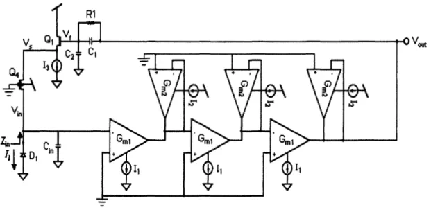
In Figure 2.7, Dl and Qi form a logarithmic photoreceptor similar to the one in Figure 2.6. Transistors Q2, Q3, and Q4 function as a single-stage inverting common-source amplifier. The cascode transistor Q4 nullifies the Miller effect on the gate-to-drain capacitance of Q2 by isolating the drain of Q2 from the large voltage swings of Vout, and also doubles the gain of the amplifier. All transistors in the circuit of Figure 2.7 operate in the subthreshold regime of operation except possibly Q2, Qs, or Q4. Cl, C2, and R1 form a temporal filter. Cl and Ci constitute a capacitive divider, and Rl is used to control adaptation in the receptor. The feedback loop is closed at the gate of Ql. The gate voltage of Ql (Vf) is determined by the feedback loop and is of a value such that all the photocurrent of Dl is supplied by Ql with the voltage Vin nearly constant. The voltage Vin is clamped to be such that the biasing current of transistor Q3 is supplied by Q2. The pinning of Vin by the transimpedance feedback loop ensures that the photodiode does not have to supply much current to charge the capacitance at the input. Thus, the extremely slow light-dependent time constant of the system is sped up via feedback. The amount of speedup increases monotonically with the feedback loop gain.
We can justify this speedup process from an alternative point of view. Note that the feedback utilized in the circuit of Figure 2.7 is a shunt-shunt feedback configuration [22]. This topology decreases the resistance seen at the input node of the sensor (i.e. l/g,1) by a factor equal to the loop gain, therefore, the input time constant which is set by this resistance gets smaller by the same factor.
At this point, let us compute the input-output I-V relationship of the photoreceptor in Figure 2.7. We know that the logarithmic I-V conversion is achieved by transistor Q1 operating in its subthreshold region with a general I-V relationship of [23], [24]
XSVGS - V m
- - In Saturation: VDS 2 5Ur - HGS
IDS = Iwe uT (1
-
e uT )>
IDS = IOe ^In this equation, Vas and Vos are the gate-to-source and drain-to-source voltages, respectively; ~ = K = \ l n is the subthreshold exponential coefficient; Ios=Io is the
subthreshold current-scaling parameter; and UpkT/q is the thermal voltage. In the simple model of (2.2), the small effect of a nonzero drain-to-source conductance on Ins (channel- length modulation) has been neglected.
Considering that the source voltage of transistor
Qi
(Vin) is clamped by the feedback loop and is nearly constant and ignoring the temporal filter for now, we can writeKl ( I * )
Equation (2.3) defines the large-signal input-output relationship of the circuit in Figure 2.7. The small-signal relationship can be obtained by differentiating equation (2.3) around each operating point
This indicates that, as mentioned before, the (small-signal) output voltage of the photoreceptor is proportional to AIl/Il or AEIE, the contrast of the input light.
On the other hand, according to equation (2.3), when the DC photocurrent increases by a factor of 10, the output voltage rises by only
(UT
/ ~ ~ ) x l n l O ~ 8 5 m V (assuming ~]=0.7). Thus, for instance, even if the ambient light intensity varies by 6 orders of magnitude from moonlight to bright sunlight, the compressive properties of logarithm assures that the voltage changes by merely 510mV, which should not cause any saturation problem. This validates that a logarithmic photoreceptor has a large dynamic range.However, as there is no free lunch in engineering, this powerful compression also causes the sensitivity (or current-to-voltage conversion gain) of a logarithmic photoreceptor to become lower than their linear counterparts. For example, as mentioned earlier, the output voltages generated by logarithmic sensors in response to small contrasts can be comparable in size with or even overwhelmed by their FPN, which are typically a few mV in magnitude. This is the reason why logarithmic sensors are not very
popular in carnera-like image sensing applications5 (which handle still images with spatial, but no temporal, variation).
However, the photoreceptor being designed in this chapter is intended for use in visual sensors which typically deal with visual scenes with temporal information (i.e. they vary in time). Consequently, we can apply a temporal solution to improve the poor conversion gain of logarithmic photoreceptors.
The solution is to use temporal filtering to boost the gain for the signals of interest
[3]. The elements Cl, C2, and Ri in Figure 2.7 form a temporal low-pass network in the feedback path, which results in an overall high-pass characteristic for the photoreceptor. The transfer characteristic of the feedback low-pass filter is easily obtained as
At low frequencies, the feedback loop is closed via Rl, while at high frequencies the feedback loop is closed via the Cl-C2 capacitive divider. Thus, the closed-loop transient or ac gain is larger than the closed-loop steady state or DC gain by a factor of (Cl+C2)/Cl. Hence, low-frequency information (including mismatches) is adapted out by the receptor6 to have a logarithmic response, while high-frequency information is amplified by the additional gain of the capacitive divider7. The photoreceptor circuit centers its operating point around the history of light intensity to simultaneously achieve higher sensitivity and wider dynamic range. These properties are consistent with our observation of the characteristics of biological photoreceptors in Section 2.1.
There have been some solutions reported in the literature to reduce the FPN of logarithmic sensors and utilize them for imaging purposes; for instance, see an on-chip electronic calibration scheme in [25] or an
off-chip mathematical calibration approach in [26]. However, these techniques either result in levels of
FPN still not suitable for high-quality imagers or add substantial complexity to the system.
'
Correlated double sampling (CDS) [27]-[28], which is commonly employed in linear image sensors to attenuate the effect of mismatches [l 11, [19], could in principle be used in our logarithmic photoreceptor as well. However, since, unlike charge-integration pixels, our photoreceptor is a continuous-time sensor with no sampling or clocking involved, we preferred to utilize a continuous-time solution to mismatch problem, like the one introduced above.7
Also, remember that matching between capacitors, if carefully laid out, is much better than the matching between threshold voltages of transistors in integrated circuits.
The resistance Ri,
Ci,
and Ci in Figure 2.7 are adjusted to yield the desired comer frequency of adaptation. A large resistance is needed to satisfy the very slow time constants required for adaptation (in the order of several seconds). This cannot be readily implemented using conventional devices or circuits. Among several devices employed by Delbmck to implement adaptive element Rl [3], aPMOS
transistor (in an n-well process) with its body terminal connected to source and its gate terminal connected to drain appears to be the most suitable one [ 6 ] , [ll]. This device also has a nontunable expansive (sinh-like) monotonic I-V curve. It essentially acts like a pair of diodes, in parallel, with opposite polarity. The current increases exponentially with large voltage (>0.6V approximately) for either sign of voltage and there is an extremely high resistance region around the origin (depending on the leakage current of the transistor which is typically in the order of fA). This characteristic ensures that large transients- say, moving from shadow into sunlight- do not cause the photoreceptor output to saturate and are dampened and adapted out quickly.In summary, under normal circumstances, the adaptive element acts like a normal and extremely large resistor, labeled Rl in Figure 2.7. The photoreceptor still has the same DC (or very-low-frequency) conversion gain given in equation (2.4), but features an additional (Ci+C2)/Cl gain for signals with frequencies beyond the adaptation frequency set by the temporal filter at l/(2nRl Ci). This pole is usually around 0. lHz which means that virtually all time-varying (ac) signals can benefit from this extra gain and boost their sensitivity. The output voltage of the photoreceptor in Figure 2.7 for these ac signals is
In our design, we have chosen the capacitive divider ratio to be around 15 after considering the trade-off involved: Cl should not be smaller than a certain limit (-50fF) to avoid being comparable to parasitic capacitances on the chip and losing its reliability and C2 cannot get too large because it loads the output and reduces the bandwidth of the sensor (at a given power consumption level). With these numbers, even a contrast of only 1% produces an output voltage of 5.5mV, which is normally not lost in the
FPN.
The loop gain of the feedback loop Alp, beyond the adaptation frequency, is [3], [6]
where Amp is the gain of the Q2-Q3-Q4 conunon-source-amplifier shown in Figure 2.7 and Aci is the closed-loop (voltage) gain of the photoreceptor. Loop gain is important in determining the amount of speed up that the slow light-dependent pole of the photoreceptor experiences and the resulting final bandwidth of the sensor.
2.3
OUR IMPROVEMENTS TO SILICON LOGARITHMIC
PHOTORECEPTORS
We discussed that the photoreceptor in Figure 2.7 is a continuous-time logarithmic sensor suitable to process light inputs with (spatio-) temporal information. We showed that this photoreceptor exhibits some of the characteristics seen in biological photoreceptors including a logarithmic DC response, a contrast response with adaptation to ambient light level, and a higher gain to ac (transient) than DC (steady) inputs. However, there is still room to enhance certain functional aspects of this photoreceptor. For instance, the simple feedback loop in the receptor and uncontrolled unwanted capacitances in its architecture limit the speedup of its light-dependent input time constant; the bandwidth of these non-clocked photoreceptors changes linearly with intensity as opposed to a fourth-root power in biological receptors; and the power is wasted most of the time because of simple biasing strategies. In this section, we present our contributions to improve the performance of existing logarithmic photoreceptors and demonstrate how these concepts are realized at circuit level.
2.3.1 Distributed (Cascaded) Amplification
A very useful technique that is widely used in biology [8] as well as in many man- made systems to enhance the gain-bandwidth product and dynamic range, is the application of distributed (cascaded) amplification stages. As evidence, let us go back to
Figure 2.3(a) in Section 2.1 and consider how the complex feedback loop utilized in the biological photoreception chain operates to prevent the saturation of the system during high light intensity levels and preserve the input dynamic range.
As we pointed out in that section, the cGMP molecules keep sodium channels in the photoreceptor membrane open and create a "dark current" that flows across the photoreceptor membrane. The radiation of light activates a PDE molecule which then reduces the amount of cGMP molecules present in the photoreceptor. As a result, the sodium current is reduced which means that ~ N A (in Figure 2.3(b)) and the membrane
potential (Vm) fall. This drop in the membrane potential is then reported to the brain.
One popular working model states that open sodium channels also allow calcium ca2* ions to enter the cell. In fact, the ratio of calcium to sodium currents is about 1 to 7. A calcium pump extrudes the incoming calcium and calcium reaches an equilibrium concentration within the cell. Figure 2.3(a) reveals that the equilibrium concentration of ca2* is determined by the integral of the difference between the incoming ca2* current and the outgoing ca2* pump current. A high light level causes a drop in the incoming ca2+ current which results in a net drop in the internal ca2* concentration within the cell. The fall in the ca2* concentration begins a cascade of feedback events in the cell whose net effect is to reduce the gain of the system to light and allow sensing of the signal without saturation.
The feedback pathway that is most well studied in the literature is shown as a solid black line in Figure 2.3(a): The reduction in ca2* concentration removes the inhibition of cGMP resynthesis by guanate cyclase. Thus, more cGMP is synthesized when the light level increases, which helps turn down the sensitivity of the cascade to light. In addition, the ca2* concentration drop also causes a decrease in the gain of the transduction cascade prior to the cGMP stage. The enzyme activity for these stages of the pathway is effectively decreased and thus their sensitivity to light drops as well [8]. In Figure 2.3(a), the feedback to these stages is marked with dotted lines. To summarize, the interaction of two state variables plays a vital role in this adaptation mechanism, the concentration of cGMP as the feedforward state variable and the concentration of calcium ca2* ions as the feedback state variable.
Figure 2.8: A cascade of amplifiers to realize an overall gain of A.
As we observe in the block diagram of Figure 2.3(a), biology has chosen to implement a cascade of gain stages rather than have a single stage of gain. To further praise this scheme, let us point out that the concept of cascaded amplifiers is also frequently used by engineers in various applications, for example, in the design of
RF
low-noise amplifiers (LNA) [29]-[30]. The reason is that it is hard to build a single-stage amplifier with a large gain-bandwidth product. On the other hand, a cascade of amplifiers, like the one shown in Figure 2.8, usually (but not necessarily always) has a significantly larger gain-bandwidth product than a single-stage amplifier with the same gain. It has been proven in [29] that if the gain-bandwidth product of each amplifying stage is constant, the time constant for the N-stage amplifier of Figure 2.8 is proportional to N'^A(~^ versus being proportional to A for the single-stage case (with the same overall gain). This result arises because, while time constants add in a cascade, gains multiply. In other words, a large gain-bandwidth product is achieved in a multistage amplifier because you can build up gain more quickly than you lose bandwidth8. As a result, bandwidth considerations help us understand why the gain might have been distributed in biological and engineering systems.
Let us clarify this concept farther with the help of a numerical example with typical numbers for our photoreceptor. Suppose that we want to realize a gain of 8000 in our amplifier to speed up a light pole that initially lies at 1Hz (while the feedback loop is
open) in a typical low light-intensity condition. Our aim is to obtain a closed-loop bandwidth at least in the kHz range, enough for most visual applications, while keeping the feedback loop reasonably stable. Suppose that first we decide to implement this gain
8
It can be shown that the optimal gain-bandwidth product is attained when all stages have a gain of ell2 and
therefore there needs to be 21nA number of gain stages to achieve a target gain of A [29]. However, to keep the power and noise performance of the amplifier under control, it is impractical to have too many gain stages.
by cascading 3 gain stages, each having a gain of 20. Assume that each amplifying stage has a gain-bandwidth product of 2x10' (in Hz). Therefore, the feedback loop has 1 open- loop light pole at IHz, 3 open-loop amplifier poles at 2x10⁶/20=100kHz, and a loop gain of 8000~. Root locus and feedback loop analysis show that when the feedback loop is closed, the light pole is moved to 1 1kHz. Also, one of the amplifier poles is transferred to 43kHz while the other two are much higher in frequency. Thus, the closed-loop system acts almost like a first-order system with a bandwidth of about 11kHz (set by the light pole) and no stability problem. This example also shows that because the light-dependent pole acts as a dominant pole for the system, there are no potential stability problems due to the existence of 3 amplifier poles in this feedback loop.
Now suppose that we want to implement the required gain by a single amplifying stage. In this case, the feedback loop has 1 open-loop light pole at lHz, a single open- loop amplifier pole at 2xl0~/8000=250~z, and a loop gain of 8000. Note that this amplifier pole is now 400 times slower than the amplifier poles above at the same overall gain, meaning that the effective gain-bandwidth product of the amplifier is smaller. When the feedback loop is closed, these two poles come together and depart the real axis and form a complex pair at a frequency of 1.4kHz and a Q of 5.6. Therefore, not only the single-stage-amplifier system has a final bandwidth of almost 8 times lower than the 3- stage one, it exhibits poor transient response and large overshoot which makes it practically unusable. This example demonstrates the merits of distributing the gain over many stages in our photoreceptor design.
In some visual sensing applications, such as pulse oximetry which will be described in Chapter 5, the bandwidth of the photoreceptor has to be kept higher than a certain level to ensure the proper function of the light sensor. Due to its limited gain-bandwidth product, a single-stage amplifier is not likely to sufficiently speed up a very slow light- dependent pole (existing in situations where the intensity of the input light is very low) to meet the bandwidth requirement of the photoreceptor while keeping its feedback loop stable. This problem is solved by employing a distributed amplifier in our photoreceptor to simultaneously achieve large values for both the gain and the bandwidth.
-
The capacitive divider in the feedback path has been ignored in this example without hurting our argument.
figure 2.9: The structure of the distributed amplifier that will be employed in our new photoreceptor.
Consequently, distributed amplification also increases the operating light intensity dynamic range of our photoreceptor in these applications.
Figure 2.9 illustrates the structure of the distributed amplifier that will replace the single-stage amplifier of Figure 2.7 in our new photoreceptor. Six operational transconductance amplifier (OTA) blocks form a 3-stage amplifierlo. These blocks have an input-output relationship defined by: iom = Gmi(vin+
-
v ~ ~ . ) ~ = ~ , ~ where Gmi is proportional to Ii. This relationship implies that the OTA2 blocks, in which the output terminal is connected to the negative input terminal, act like resistors of value l/Gnc. Thus, the total gain of the 3-stage amplifier is (-Gml/Gna)'.By employing some feedback linearization techniques such as source or gate degeneration or the use of the well as an input [31], Gm? can be designed to have a value many times smaller than Gnu at the same bias current, thus increasing the overall gain of our distributed amplifier. The circuit implementations of the specific OTAl and OTA2 blocks utilized in our design are displayed in Figure 2.10. OTAl is a cascode differential amplifier with active load. OTA2 is a wide output voltage range differential amplifier
[23] that uses the well (body) terminals of the two input PMOS transistors, instead of
their gates, to lower the transconductance of the block (i.e. Gna) and increase its linear range. Remember that in both subthreshold or above-threshold regions, the well terminal of a transistor has a weaker effect (gmb) in generating current compared to its gate
10
As we will show in Section 2.5, the noise of our distributed amplifier is negligible compared to the shot noise of typically small photocurrents sensed by the photoreceptor.
"out
Figure 2.10: Circuit implementations of (a) OTA1 blocks and (b) OTA2 blocks utilized in the distributed amplifier of Figure 2.9 (All the transistors have W=L=4.8pm).
terminal (gm). For example, in a subthreshold MOS transistor, g m ^ w T and gmbZ(l-
K)I~~/U~
(K
is greater than 0.5). The values of Gmi and Gm2 are equal to gm of the inputtransistors in Figure 2.10(a) and gmb of the input transistors in Figure 2.10(b), respectively.
2.3.2
Automatic Loop Gain ControlApart from distributed amplification, one other feature that stands out in the operation of the sophisticated biological feedback system of Figure 2.3(a) is the application of gain control. In subsection 2.3.1, we said that the concentration of calcium ions, as a feedback variable, controls and adapts the gain of the system to light; for example, it causes a reduction in the gain when there is high (bright) light level and hence facilitates sensing of the input signal without saturation.
To supply further evidence, let us now consider another important property observed in biological receptors, i.e. rapid response time, invariant to lighting conditions. Biological photoreceptors have a bandwidth that is practically invariant to light level, over a wide range of intensities. In toad rods, for example, the bandwidth goes as the fourth root of intensity, as shown in Figure 2.1 1 [ 6 ] . This behavior means that over a factor of 200 in background intensity, the response latency to a flash of light varies by
Gain (arbitrary units)
Figure 2.11: Time to peak response (to a flash of light) versus gain, in toad rod photoreceptors.
only a factor of about 4. There are many possible hctional reasons for this invariance. For example, we can speculate that this invariance is usehl for dynamic visual processing of moving images, or perhaps to control power consumption, or possibly to control noise. The bandwidth-invariant characteristic of biological receptors is usually attributed to the employment of distributed amplification and gain control in their complex feedback systems.
In any case, this quality suggests that we should also strive to build a receptor circuit with response speed as invariant to light illumination as possible. In our silicon photoreceptors, this speed is related to the closed-loop bandwidth of the circuit. As previously mentioned, in the transimpedance logarithmic photoreceptor topologies considered in this chapter, the closed-loop bandwidth is primarily set by the feedback loop gain of the receptor (assuming fast amplifier poles) which itself depends on the gain of the amplifier (refer to equation (2.7)). Unfortunately, in the state-of-the-art logarithmic photoreceptor of Figure 2.7, since the gain of the single-stage amplifier is fixed regardless of the light level, the bandwidth changes linearly with light intensity, which is much more severe than biology. Even the gain of the distributed amplifier shown in Figure 2.9 is constant unless a mechanism to change and control the gain is put in place.
Indeed f?om a pure engineering point of view, adapting the amplifier gain in our photoreceptor topology also makes sense. This is to keep the stability of the sensor under control without an excessive increase in its power consumption. To better understand this
Gain Control Circuitry
m
Distributed AmplifierFigure 2.12: The circuit schematic of a logarithmic photoreceptor with distributed amplification and automatic loop gain control (All the transistors seen in this figure have
W=L=4.8pm).
point, we reconsider the numerical example given in subsection 2.3.1 for a photoreceptor with a 3-stage distributed amplifier. Suppose that with the same loop gain (8000) and the same 3 amplifier poles (at lOOkHz), the input light intensity striking the photoreceptor increases by a factor of 1000 (for example, the sensor is moved fiom an outdoor moonlit ambient into an indoor ofice room). This causes the new open-loop light pole to move to 1kHz. Feedback loop analysis shows that when the loop is closed, two of the poles move to the right half of the real-imaginary plane and the photoreceptor becomes unstable. One solution to this problem is to burn considerably more power and move the amplifier poles to a much higher location than 100kHz to avoid instability. The bad news is that this extra power is being wasted most of the time when photoreceptor is dealing with light intensities lower than the maximum level it is designed to sense.
A better power-saving solution to prevent instability is to reduce the loop gain of the photoreceptor when input light level gets high while still maintaining a large loop gain when the light level is low so that the sensor achieves a certain speed in both cases. For instance, in the above example, if the loop gain is decreased to 8 when the input light increases by 1000, the closed-loop system will have a dominant pole at 13kHz (still