Ambient Noise Tomography for Wavespeed and
Anisotropy in the Crust of Southwestern China
by
Hui Huang
M.S. Geophysics, Peking University, Beijing, China, 2007 B.S. Geophysics, Peking University, Beijing, China, 2004
Submitted to the Department of Earth, Atmospheric, and Planetary Sciences
A
I
in partial fulfillment of the requirements for the degree ofDoctor of Philosophy at the
MASSACHUSETTS INSTITUTE OF TECHNOLOGY
MASSACHUSETTS INSTIWE OF TECHNOLOGY
MAR03 2014
LI LIBRARIES
February 2014©2014 Massachusetts Institute of Technology. All rights reserved
Author:...
Depart ent of Earth, Atmospheric, and Planetary Sciences October 11, 2013 Certified by:... .. .x...
Robert D. van der Hilst Schlumberger Professor of Earth Sciences Head, Department of Earth, Atmospheric and Planetary Sciences Thesis Supervisor Accepted by:...
Robert D. van der Hilst Schlumberger Professor of Earth Sciences Head, Department of Earth, Atmospheric and Planetary Sciences
Ambient Noise Tomography for Wavespeed and
Anisotropy in the Crust of Southwestern China
by Hui Huang
Submitted to the Department of Earth, Atmospheric, and Planetary Sciences on October 11, 2013 in partial fulfillment of the requirements for the Degree of
Doctor of Philosophy in Geophysics
Abstract
The primary objective of this thesis is to improve our understanding of the crustal structure and deformation in the southeastern Tibetan Plateau and adjacent regions using surface wave tomography. Green's functions for Rayleigh and Love waves are extracted from ambient noise interferometry. Using the Green's functions, we first conduct traditional traveltime tomography for the two shear wavespeeds Vsv and VSH Their differences are measured as radial anisotropy. We then conduct Eikonal tomography to study azimuthal anisotropy in the crust. Our tomography results are well consistent with geology in the study region. In the Sichuan Basin, low wavespeed and positive radial anisotropy (VsH> Vsv) in the upper crust reflect thick sedimentary layers at surface; high wavespeed and small radial anisotropy in the middle and lower crust reflect a cold and rigid basin root. Little azimuthal anisotropy is observed in the Basin, indicating small internal deformation. In the Tibetan Plateau, we observe widespread low wavespeed zones with positive anisotropy in the middle and lower crust, which may reflect combined effects of weakened rock mechanism and horizontal flow in the deep crust of southeastern Tibet. The northern part of the Central Yunnan block, which geographically coincides with the inner zone of the Emeishan flood basalt, reveals relatively higher wavespeeds than the surrounding regions and little radial anisotropy throughout the entire crust. We speculate that the high wavespeeds and small radial anisotropy are due to combined effects of the remnants of intruded material from mantle with sub-vertical structures and channel flow with sub-horizontal structures. In general, the azimuthal anisotropy in our study region is consistent with a clockwise rotation around the Eastern Himalayan Syntaxis. Careful examination reveals large angular differences between the azimuthal anisotropy in the upper and lower crust, suggesting different deformation patterns at the surface and in depth. Therefore, our tomography results support models with ductile flow in the deep crust of the southeastern Tibetan Plateau; however, the large lateral variation of both wavespeeds and anisotropy indicates that the flow also varies greatly in intensity and pattern in different geological units.
Thesis supervisor: Robert D. van der Hilst Title: Schlumberger Professor of Earth Sciences
Acknowledgments
First of all, I would like to express my heartfelt gratitude to my advisor Professor Robert D. van der Hilst for his invaluable advice and guidance. He showed unlimited patience in our discussion. This work could not have been done without his interests and encouragement. He always unselfishly contributed his creative ideas, which constantly helped me out of troubles and pushed me towards brighter directions in the research. His enthusiasm about Earth sciences had great influence in my MIT life. Through him, I understood what it means to be a geophysicist. It was my greatest fortune and pleasure to work with him.
I owe much gratitude to Professor Brad Hager, who was the advisor for my second project in general exam. He always made time to answer my questions and offer useful insights. I also owe much to Professor Maarten de Hoop at Purdue University. His broad knowledge in geophysics and mathematics was particularly helpful for my research. I would also like to thank other thesis committee members Professor Leigh Royden, Professor Alison Malcolm, and general exam committee member Professor Nafi Toks6z. Conversations with them were very useful for my research.
My appreciation also goes to Professor Huajian Yao from University of Science and Technology of China, Professor Qiyuan Liu and Dr. Yu Li from the China Earthquake Administration. The precious collaboration with them was invaluable to the project.
My work was also benefited by intuitive discussion with Research Scientists, Postdocs, and graduate students at EAPS, Ping Wang, Min Chen, Xuefeng Shang, Tianrun Chen, Zhenya Zhu, Chang Li, Haijiang Zhang, Yingcai Zheng, Rizheng He, Junlun Li, Xinding Fang, Di Yang, Chen Gu, Chunquan Yu, Jing Liu, Haoyue Wang, and Zhulin Yu.
I would also like to thank Sue Turbak, Vicki McKenna, Carol Sprague, and Jacqueline Taylor for their constant help during my six years at MIT.
I am deepest grateful to my husband Jian Yang, my mother Gaoxiu Jia and my sister Shengnan Huang for their greatest support, encouragement and love.
Table of Contents
A bstract ... 3
A cknow ledgm ents ... 5
List of Figures... 9
C hapter 1 Introduction... 11
1.1 Structure and deformation in the lithosphere of the southeastern Tibetan Plateau... 11
1.2 Thesis objectives... 14
1.3 Traditional and Eikonal tom ography ... 15
1.4 Thesis structure ... 16
References...19
Chapter 2 Radial anisotropy in the crust of SE Tibet and SW China from am bient noise interferom etry ... 23
Abstract ... 23
2.1 Introduction... 24
2.2 D ata and m ethod ... 26
2.3 Shear wave velocity structure and radial anisotropy ... 27
2.4 D iscussion and conclusions ... 28
Appendix 2A ... 30
Appendix 2B ... 33
A cknow ledgm ents... 34
References...35
Chapter 3 High resolution tomography and radial anisotropy of SE Tibet and its surrounding regions using ambient noise interferometry...55
Abstract ... 55
3.1 Introduction... 56
3.2 Seism ic noise data and interferom etry... 58
3.3 Phase velocity inversion ... 59
3.4 Shear wave speed inversion... 61
3.4.1 Inversion schem e ... 61
3.4.2 Param eter setting ... 63
3.4.3 Inversion exam ples ... 65
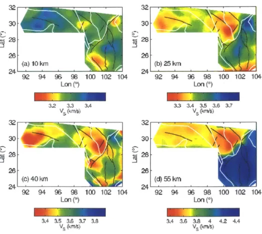
3.5 Three-dimensional structure of shear wave speed and radial anisotropy ... 66
3.5.1 Shear w ave speed structure ... 66
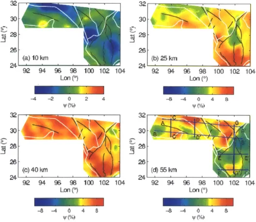
3.5.2 Radial anisotropy ... 69
3.6 D iscussion... -... ... ... ... 70
3.6.1 Sichuan Basin... 70
3.6.2 Tibetan Plateau... 72
3.7 Sum m ary and conclusions ... 76
References...78
Chapter 4 Eikonal tomography and azimuthal anisotropy for the SE Tibet and SW China...99
Abstract ... .... 99
4.1 Introduction... 100
4.2 Eikonal tom ography...102
4.2.1 Ambient noise data and Rayleigh wave Green's function...102
4.2.2 Eikonal equation ... 103
4.2.3 Minimum curvature interpolation...104
4.2.4 D am ping and sm oothing in interpolation ... 107
4.3 Phase velocity and anisotropy m aps ... 108
4.3.1 A zim uthal anisotropy at a single location... 108
4.3.2 Resolution test... 109
4.3.3 Phase velocity and anisotropy m ap... 111
4.4 Shear w ave speed and anisotropy ... 112
4.4.1 N A inversion for anisotropic m odel... 112
4.4.2 The 3-D heterogeneity and azimuthal anisotropy... 114
4.5 D iscussion ... 117
4.5.1 Phase velocity maps from Eikonal and traditional tomography .... 117
4.5.2 Azim uthal and radial anisotropy... 118
4.5.3 Comparison with GPS and shear-wave splitting ... 122
4.6 Conclusions...123
Appendix 4A ... 124
Appendix 4B ... 126
References...128
C hapter 5 Concluding rem arks ... 155
5.1 Sum m ary ... 155
5.2 Future w ork... 159
List of Figures
Figure 1-1 Seismic stations used in the thesis ... 22
Figure 2-1 Seismic stations used in this study... 37
Figure 2-2 Examples of inversion at different locations... 38
Figure 2-3 Radial anisotropy ... ... 39
Figure 2-4 Vertical profiles for Vsv and Radial anisotropy... 40
Figure 2-5 Statics analysis for Vsv and radial anisotropy ... 41
Figure 2A-1 Band-pass filtered EGFs ... 42
Figure 2A-2 Variations of shear wavespeeds... 43
Figure 2A-3 Tradeoffs between radial anisotropy and Moho depth... 44
Figure 2A-4 Color codes for main tectonic units in our study area...45
Figure 2A-5 Statics analysis for VsH and radial anisotropy ... 46
Figure 2A-6 Relationship between Vsv anomaly and VsH anomaly ... 47
Figure 2B-1 Seismic stations used in this study ... 48
Figure 2B-2 Variations of Vsv ... 49
Figure 2B-3 Variations of radial anisotropy ... 50
Figure 2B-4 Vertical profiles for perturbed Vsv... 51
Figure 2B-5 Vertical profiles for radial anisotropy... ... 52
Figure 2B-6 Statics analysis for shear wavespeeds and radial anisotropy... 53
Figure Figure Figure Figure Figure Figure Figure Figure Figure Figure Figure Figure Figure Figure Figure Figure Figure 3-1 3-2 3-3 3-4 3-5 3-6 3-7 3-8 3-9 3-10 3-11 3-12 3-13 3-14 3-15 3-16 3-17 Seismic stations used in this study... ... 81
Transverse-component raypaths and CFs... 82
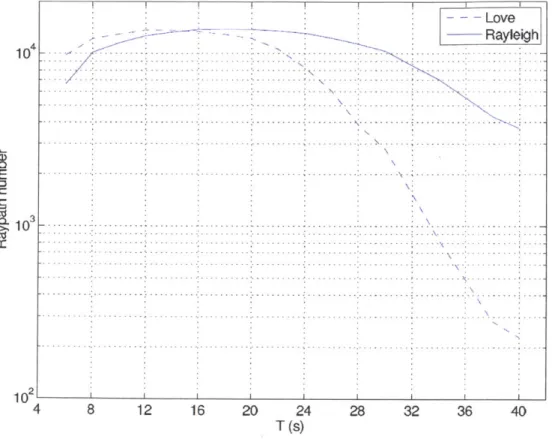
Numbers of measurements... 83
R aypath coverage... 84
Checkerboard test results... 85
Variations of phase velocity... 86
Posterior errors for phase velocity inversion... 87
L-curve analysis for shear wavespeed inversion... 88
D ata m ism atch... 89
Examples of inversion in different tectonic units... 90
Variations of Vsv at four depths... ... 91
Variations of VsH at four depths... 92
Variations of radial anisotropy at four depths... 93
Standard deviations for the radial anisotropy... 94
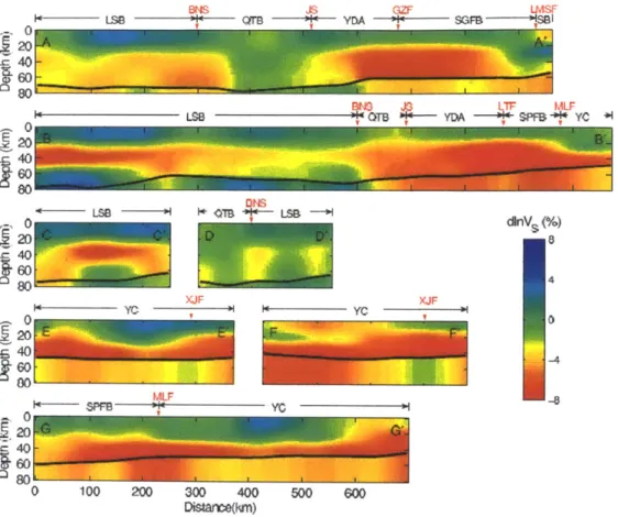
Vertical profiles for perturbed Vsv... 95
Vertical profiles for radial anisotropy... 96
Figure 4-2 Raypaths and CFs...133
Figure 4-3 Numbers of measurements...134
Figure 4-4 Traveltime from one virtual source station...135
Figure 4-5 Perturbed traveltime...136
Figure 4-6 Phase velocity maps calculated from the traveltime...137
Figure 4-7 Phase velocity against the propagation direction...138
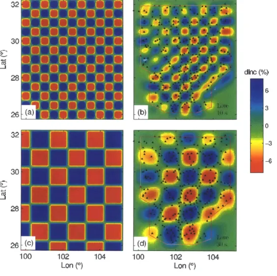
Figure 4-8 Checkerboard test for isotropic phase velocity...139
Figure 4-9 Checkerboard test for azimuthal anisotropy...140
Figure 4-10 Eikonal tomography results for 10 s Rayleigh wave ... 141
Figure 4-11 Eikonal tomography results for 30 s Rayleigh wave...142
Figure 4-12 Variations of Vsv and azimuthal anisotropy...143
Figure 4-13 Standard errors for Vsv...144
Figure 4-14 Standard errors for azimuthal anisotropy...145
Figure 4-15 Angular differences of anisotropy between crustal layers...146
Figure 4-16 Comparison of azimuthal anisotropy and SKS splitting ... 147
Figure 4A-1 Test of anisotropy for 10 s Rayleigh wave...148
Figure 4A-2 Artificial azimuthal anisotropy from checkerboard model ... 149
Figure 4A-3 Artificial azimuthal anisotropy from realistic model...150
Figure 4B- 1 Love wave phase velocities...151
Figure 4B-2 Test of anisotropy for 10 s Love wave ... 152
Figure 4B-3 Eikonal tomography results for 10 s Love wave ... 153
Chapter 1
Introduction
1.1 Structure and deformation in the lithosphere of the southeastern Tibetan Plateau
The Tibetan plateau, as the consequence of the collision between the Indian and
Eurasian plates, has elevated more than 5km since about 50 Ma (Molnar and Tapponnier, 1975). As the Indian plate moves northward, materials are extruded from the central collision zone to the margins of the Plateau, causing rapid surface uplift of southeastern Tibet at approximately 8 Ma (Royden et al., 2008). Due to the obstacle of the rigid lithosphere of the Sichuan Basin, this material transport bifurcates at the eastern margin of the Plateau. The southern branch changes its direction about 900 around the Eastern Himalayan Syntaxis: from nearly eastward to nearly southward (Wang, 1998; Wang and Burchfiel, 2000; Shen et al., 2005). The active material transport and lateral variation in strength of the crust cause a lot of earthquakes in the southeastern Tibetan Plateau and Central Yunnan block, including the 2008 Wenchuan earthquake (M = 8.0) on the Longmenshan fault. Therefore, the region between the Eastern Himalayan Syntaxis and the Sichuan Basin is of particular importance to understand the uplift history and relevant dynamic processes of the whole Plateau,
and our study of the crustal structure may also help understand the mechanism of the local seismicity.
The southeastern Tibetan Plateau has a complicated tectonic history (Royden et al., 2008). Even after decades of research there is still controversy and debate about the
mechanism of deformation. A lot of modeling works have been conducted to account for the topography variation, surface velocity field from GPS observations, stress field derived from earthquake focal mechanism, and other measurements. In general, there are three schools of modeling which propose distinct lithospheric settings and thus have different implications for the deformation mechanism.
The first school considers the lithosphere of Tibet as a rigid plate, and one representative example is the rigid block extrusion model (Molnar and Tapponnier, 1975; Pelzer and Tapponnier, 1988). This model proposes that the crust of Tibet is
composed of several rigid sub-blocks which have little interior deformation. Large deformation only occurs on narrow zones between these sub-blocks, which can penetrate through the entire lithosphere, to compensate the material extrusion due to the India-Eurasia collision. Since this rigid block model suggests mechanically strong and coupled lithosphere, the variation of the deformation is small in the depth direction.
that the vertical gradients of the horizontal velocity are negligible, both the rheology and modeled deformation are the averages in depth direction.
The third school proposes to explain the topography with either sharp or smooth gradient near the margins of the Tibetan Plateau (Royden et al., 1997; Clark and Royden, 2000). Channel flow with constant material transportation and deformation mainly occurs in a week zone in the deep crust and form distinct topography gradients due to the rheology contrasts between the Plateau and its surrounding regions. Since the most straightforward way to reduce viscosity is the increased temperature, we would expect, for instance, higher heat flow, lower seismic wavespeed, and higher Poisson's ratio.
Besides the above three schools with simple concepts, more complicated numerical modeling has been conducted recently (Copley and McKenzie, 2007; Copley, 2008). Since the rheology is poorly constrained, even if the deformation at the surface is well modeled its patterns in deep lithosphere can differ greatly with different settings of rheology. Therefore, the coupling of the lithosphere may not be determined from surface observations alone.
Previous studies reveal complicated variations of the material properties in the lithosphere of the southeastern Tibetan Plateau, corresponding to the complicated tectonic history of this region. These results have been used to support one of the models mentioned above. At surface, GPS observations reveal several sub-blocks separated by faults on which the major deformation occurs (Shen et al., 2005). At depth, although a weak middle and lower crust is suggested by recent discoveries of
low wavespeed zones (Yao et al., 2008, Zhang et al., 2012), high Poisson's ratio (Hu et al., 2005; Xu et al., 2007), high heat flow (Hu et al., 2000), and low electrical resistivity (Bai et al., 2010), all these properties reveal great spatial variation, both horizontally and vertically. Hence, the deformation in the deep crust, for example flow as suggested in the channel flow model (Royden et al., 1997), if it occurs at all, is also expected to vary greatly in pattern. Furthermore, based on the comparison between GPS observations and shear wave splitting, Sol et al. (2007) suggest a strong lower crust and hence couple lithosphere around the Eastern Himalayan Syntaxis but possible weak lower crust and decoupled lithosphere in southeastern Plateau.
1.2 Thesis objectives
In view of the above background, the objective of this thesis is to obtain detailed models of seismic wavespeed and anisotropy, both radial and azimuthal, to understand the deformation in the crust of the southeastern Tibetan Plateau and its surrounding regions. Firstly, we construct 3-D models for the two shear wavespeeds Vsv and VSH with vertical and horizontal polarizations, respectively, and their difference are measured as the radial anisotropy. Secondly, we investigate the relationship between
1.3 Traditional and Eikonal tomography
To meet the objectives above, we conduct both traditional and Eikonal tomography on surface wave signals extracted from ambient noise interferometry (Yao et al., 2006). The Green's functions for both Rayleigh and Love waves are calculated from cross-correlation functions of the seismic noise records. We use data from three temporary arrays in the southeastern marginal region of the Tibetan Plateau and the Sichuan Basin (Figure 1-1). Two relatively sparse arrays were deployed by Lehigh University and Massachusetts Institute of Technology (MIT) from Oct 2003 to Sep 2004, with an average inter-station distance of approximately 50-100 km. A much denser array was conducted by China Earthquake Administration (CEA) from Jan 2007 to Dec 2009, with an average inter-station distance of approximately 20-30 km.
In this study we only use seismic records of the year 2007 from the CEA array, because one year data is sufficient to extract clear signals of Green's functions (Bensen et al., 2007). Since Green's functions are extracted for each station-pair, we obtain very dense raypath coverage and thus tomography results with sufficient details for the study region.
The fundament of traveltime tomography is the (non-linear) relation between the traveltime of a certain wave and local wavespeed. Basically, there are two types of equations connecting them, based on which different tomography schemes are developed (Table 1). The first type of equation has an integral form: the total traveltime is the integration or summation the local wave slowness along the raypath. A kernel can be introduced into the integration to account for effects such as finite
frequency (Dahlen et al., 2000). Most of the tomography studies are based on this integration relation. A "de-integration" operation, matrix inversion in this study, can be implemented to calculate the local wavespeed. Since all the raypaths are used simultaneously in the matrix inversion, the traditional tomography has good resolution. Therefore, in this thesis, we use it to study the isotropic wavespeeds, i.e. Vsv and VsH. Radial anisotropy is also studied because it is calculated from the two
isotropic wavespeeds.
The second type of equation, i.e. the Eikonal equation, has a differential form: the local wave slowness and propagation direction are directly obtained from the gradient of the traveltime (Shearer, 1999). Eikonal tomography is more efficient in computation because it avoids the time-consuming calculation of matrix inversion in traditional tomography, especially when there are a large number of raypaths. To accurately estimate the traveltime and its gradient from a specific source for the entire study region, an interpolation operator is applied. In the interpolation, only traveltime data for the specific source are used, this procedure is fast because less data (than the whole data set) are involved. Furthermore, since no assumption is made for the raypath, the wave propagation direction is more accurate than that in the traditional tomography (great circle in this thesis). Therefore, we mainly apply the Eikonal
background geological settings for the southeastern Tibetan Plateau. We also present the motivations and objectives of this thesis work.
In Chapter 2, published as Huang et al. (2010), we conduct surface wave tomography using seismic noise records from MIT and Lehigh arrays. Green's functions for both Rayleigh and Love waves are calculated from the cross-correlation functions of the vertical and transverse components, respectively. Average phase velocities or dispersion curves along the raypaths are then measured using a phase image analysis technique (Yao et al., 2006). These dispersion curves are used to invert for 3-D models for the two shear wavespeed Vsv and VsH, respectively. The difference between the two wavespeeds are examined both in view of non-uniqueness of tomographic solutions and radial anisotropy. We also analyze the correlation between the wavespeeds and radial anisotropy.
In Chapter 3, which is in preparation for publication, we conduct surface wave tomography using seismic noise records from CEA array. This is an extension work of Chapter 2 but with much denser data and a more sophisticated inversion scheme. The densely deployed array enhances the resolution with more details for the study region. To constrain the wavespeeds and radial anisotropy better, we develop a new scheme to invert jointly for the two wave speeds (VsH and Vsv), thus the radial anisotropy is explicitly included in the inversion.
In Chapter 4, which is also in preparation for publication, we conduct Eikonal tomography (Shearer, 1999) using seismic records from CEA array as in Chapter 3. We develop an improved interpolation scheme to accurately estimate the traveltime
for Rayleigh waves, the gradient of which reflects the local wave slowness and propagation direction. Assuming a HTI medium (horizontal transverse isotropic), we obtain the angular variation of the wavespeed (or slowness) in the horizontal plane, i.e. the azimuthal anisotropy. Then the variations of azimuthal anisotropy at different depths are carefully examined and compared with surface strain-rate and SKS splitting to build up comprehensive perspectives about the crustal deformation for the southeastern Tibetan Plateau.
Chapter 5 is the summary and conclusion chapter. We summarize our understanding of the structure and deformation mechanism in the lithosphere of the southeastern Tibetan Plateau. Possible directions of future research are also discussed.
References
Bai, D., M. J. Unsworth, M. A. Meju, X. Ma, J. Teng, X. Kong, Y. Sun, J. Sun, L. Wang, C. Jiang, C. Zhao, P. Xiao, and M. Liu, (2010), Crustal deformation of the eastern Tibetan plateau revealed by magnetotelluric imaging, Nature Geosci., 3,
358-362, doi:10.1038/ngeo830.
Bensen, G.D., M.H. Ritzwoller, M.P. Barmin, A.L. Levshin, F. Lin, M.P. Moschetti, N.M. Shapiro, and Y. Yang, (2007), Processing seismic ambient noise data to obtain reliable broad-band surface wave dispersion measurements, Geophys. J. Int., 169, 1239-1260.
Clark, M., and L. Royden, (2000), Topographic ooze: Building the eastern margin of Tibet by lower crustal flow, Geology, 28, 703-706.
Copley, A., D. McKenzie, (2006), Models of crustal flow in the India-Asia collision zone, Geophys. J. Int., 169, 683-698.
Copley, A., (2008), Kinematics and dynamics of the southeastern margin of the Tibetan Plateau, Geophys. J. Int., 174, 1081-1100.
Dahlen, F., S. Huang, and G. Nolet, (2000), Frechet kernels for finite-frequency traveltimes - I. Theory, Geophys. J. Int., 141(1), 157-174.
England, P., and D. McKenzie, (1982), A thin viscous sheet model for continental deformation, Geophys. J. R. Astr. Soc., 70, 295-321.
England, P., and G. Houseman, (1986), Finite strain calculations of continental deformation, 2, Comparison with the India-Asia collision zone, J. Geophys. Res.,
91, 3664-3676.
Flesch, L., J. Haines, W. Holt, (2001), Dynamics of the India-Eurasia collision zone, J. Geophys. Res., 106(B8), 16435-16460.
Hu, S., L. He, and J. Wang, (2000), Heat flow in the continental area of China: a new data set, Earth planet. Sci. Lett., 179, 407-419.
Hu, J.F., Y.J. Su, X. Zhu, Y. Chen, (2005), S-wave velocity and Poisson's ratio structure of crust in Yunnan and its implication, Science in China Ser. D Earth Sciences, 48(2), 210-218.
Huang, H., H. Yao, and R.D. van der Hilst (2010), Radial anisotropy in the crust of SE Tibet and SW China from ambient noise interferometry, Geophysical Research Letters, 37(21), DOI: 10.1029/201 0GLO4498 1.
Molnar P., and P. Tapponnier, (1975), Cenozoic tectonics of Asia: Effects of a continental collision: Features of recent continental tectonics in Asia can be interpreted as results of the India-Eurasia collision, Science, 189, 419-426. Peltzer, G., and P. Tapponnier, (1988), Formation and evolution of strike-slip faults,
rifts, and basins during the India-Asia collision: An experimental approach, Journal of Geophysical research, 93, 15085-15117.
Shearer P., (1999), Introduction to seismology, Cambridge University Press, ISBN
0-521-66023-8 (hbk.).-ISBN 0-521-66953-7 (pbk), 237-240.
Royden, L.H., B.C. Burchfiel, R.W. King, E. Wang, Z. Chen, F. Shen, and Y Liu, (1997), Surface deformation and lower crustal flow in eastern Tibet, Science, 276,
Royden, L.H., B.C. Burchfiel, R.D. van der Hilst, (2008), The geological evolution of the Tibetan plateau, Science, 321, 1054-1058.
Shen, Z., J. Lv, M. Wang, R. Burgmann, (2005), Contemporary crustal deformation around the southeast borderland of the Tibetan Plateau, Journal of Geophysical research, 110, B 11409.
Sol, S., A. Meltzer, R. Burgmann, R.D. van der Hilst, R. King, Z. Chen, P.O. Koons, E. Lev, Y.P. Liu, P.K. Zeitler, X. Zhang, J. Zhang and B. Zurek, (2007), Geodynamics of the southeastern Tibetan Plateau from seismic anisotropy and geodesy, Geology, 35, 563-566.
Wang, E., (1998), Late Cenozoic Xianshuihe-Xiaojian, Red River and Dali fault systems of southwestern Sichuan and central Yunnan, China, Spec. Pap, Geol.
Soc, Am., 327.
Wang, E., B.C. Burchfiel, (2000), Late Cenozoic to Holocene deformation in southwestern Sichuan and adjacent Yunnan, China, and its role in formation of the southeastern part of the Tibetan Plateau, Geol. Soc. Am. Bull., 112, 413-423. Xu, L., S. Rondenay, and R. D. van der Hilst, (2007), Structure of the crust beneath
the southeastern Tibetan Plateau from teleseismic receiver functions, Phys. Earth Planet. Int., 165, 176-193, doi: 10.1016/j.pepi.2007.09.002.
Yao, H., R. D. van der Hilst, and M. V. De Hoop, (2006), Surface-wave array tomography in SE Tibet from ambient seismic noise and two-station analysis - I. Phase velocity maps, Geophys. J. Int., 166, 732-744, doi:
10.111 1/j.1365-246X.2006.03028.x.
Yao, H., C. Beghein, and R.D. Van der Hilst, (2008), Surface wave array tomography in SE Tibet from ambient seismic noise and two-station analysis - II. Crustal-and upper-mantle structure, Geoohys. J. -Int., 173, 205-219.
Zhang, H., S. Roecker, C.H. Thurber, and W. Wang (2012), Seismic Imaging of Microblocks and Weak Zones in the Crust Beneath the Southeastern Margin of the Tibetan Plateau, Earth Sciences, Dr. Imran Ahmad Dar (Ed.), ISBN: 978-953-307-861-8, 159-202.
1-1: Comparison of traditional and Eikonal tomography
Traditional tomography Eikonal tomography Equation
t(r, r,)
f
r Vt(r,r,)= kc(r) c(r)
Wavespeed calculation Matrix inversion Interpolation and derivation
Advantage Good resolution; Fast;
Well-developed Accurate direction Application in this thesis Isotropic Vsv and VSH; Azimuthal anisotropy
Radial anisotropy
Here t(r, r) is the traveltime from source r, to location r, c(r) is the local wavespeed, and k is the unit vector along wave propagation direction.
32 28 rt 8er 2 24-90 92 94 96 98 100 102 104 106 Lon ( )
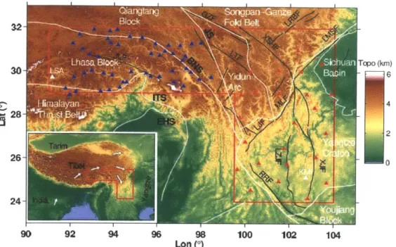
Figure 1-1. Topography, geological units and seismic stations used in this thesis. The topography is represented by the background color. The locations of seismic stations are depicted as black, red, and blue triangles for Lehigh, MIT, and CEA arrays, respectively. The two permanent stations KMI and LSA are depicted as white triangles. The white curves depict the boundaries of the geological units: Lhasa block, Qiangtang block, Yidun Arc, Songpan-Ganze fold belt and Yangtze Craton including the Sichuan Basin. Major faults are depicted as thin black lines and the abbreviations are: Ganze fault (GZF), Longriba fault (LRBF), Xianshuihe fault (XSHF), Longmenshan fault (LMSF), Longquan fault (LQF), Litang fault (LTF), Chenzhi fault (CZF), Lijian fault (LJF), Muli fault (MLF), Anninghe fault (ANHF), Zemuhe fault
(ZMHF), Xiaojiang fault (XJF), Shimian fault (SMF), and Luzhijiang fault (LZJF)
(after Wang et al., 1998; Wang and Burchfiel, 2000; Shen et al., 2005). Other abbreviations are: Eastern Himalayan Syntaxis (EHS), Jingsha Suture (JS), Bangong-Nujiang Suture (BNS), and Indus-Tsangpo Suture (ITS). The inset shows
Chapter 2
Radial anisotropy in the crust of SE Tibet and SW
China from ambient noise interferometryl
Abstract
We use Rayleigh and Love wave Green's functions estimated from ambient seismic noise to study crustal structure and radial anisotropy in the tectonically complex and seismically active region west of the Sichuan Basin and around the Eastern Himalaya Syntaxis. In agreement with previous studies, low velocity zones are ubiquitous in the mid-lower crust, with substantial variations both laterally and vertically. Discrepancies between 3-D shear velocity from either Rayleigh (Vsv) or Love (VsH) waves are examined both in view of non-uniqueness of tomographic solutions and radial anisotropy. Low shear wave speed and radial anisotropy with VsH>
Vsv are most prominent in mid-lower crust in area northwest to the Lijiang-Muli fault
and around the Red River and Xiaojiang faults. This anisotropy could be caused by sub-horizontal mica fabric and its association with low velocity zones suggests mica alignment due to flow in deep crustal zones of relatively low mechanical strength.
Published as (except Appendix 2B): Huang, H., H. Yao, and R. D. van der Hilst, (2010), Radial anisotropy in the crust of SE Tibet and SW China from ambient noise
2.1 Introduction
Despite decades of research, the mechanism of crustal deformation and eastward expansion of the Tibetan Plateau are still under debate. As the conjunction between the Tibetan Plateau and the Yangtze Indo-China blocks and the southern end of the trans-China seismicity belt, SE Tibet is of particular interest. GPS data (Zhang et al., 2004; Shen et al., 2005) and geological studies (Wang, 1998; Wang and Burchfiel, 2000) show that in this region the upper crust rotates clockwise around the Eastern Himalayan Syntaxis. But how this surface motion is related to deformation at larger depth is not yet known.
Along with geological data, including constraints on shortening and uplift history, the topography of this region - in particular, the gentle slope from ~5 km on the Plateau to less than 1 km in the southeast and the steep margin west of the Sichuan Basin - was used by Royden et al. (1997) to argue for flow in the deep crust. The area
is intersected, however, by major fault systems, such as the Red River, Lijiang-Muli, Xianshuihe-Xiaojiang, and Longmenshan faults (Figure 2-1), which seismicity and GPS measurements (Shen et al., 2005) indicate are active block boundaries. These
observations mostly pertain to the (near) surface, and more direct information about the deeper crust is needed to understand the large scale deformation this region.
mechanically weak. Furthermore, the change in pattern of azimuth anisotropy from upper crust to upper mantle (Yao et al., 2010) suggests that the crust and mantle deform differently. These inferences are qualitatively consistent with ductile flow in the deep crust (Royden et al., 1997, 2008). On the other hand, the edges of some
LVZs seem to coincide with faults (Yao et al., 2008, 2010) where GPS data reveal large slip rates (Shen et al., 2005). Combined, these observations suggest that the tectonic evolution and deformation of SE Tibet is influenced by the juxtaposition of crustal blocks with or without weak zones, separated by major faults (Yao et al., 2010).
Radial anisotropy, that is, the difference in propagation speed of horizontally and vertically polarized waves - inferred, respectively, from Love and Rayleigh wave data
- has been used to diagnose specific styles of crustal deformation (Shapiro et al., 2004; Moschetti et al., 2010). For example, crustal flow can produce a horizontal mica fabric, which, in turn, can produce significant radial anisotropy (e.g., Weiss et al., 1999; Shapiro et al., 2004). Following our work on crustal heterogeneity and
azimuthal anisotropy in the southeastern margin of Tibet (Yao et al., 2008, 2010), we determine radial anisotropy from ambient noise tomography (e.g., Shapiro et al., 2005; Yao et al., 2006) with empirical Green's functions (EGFs) for short- and intermediate period Rayleigh and Love wave propagation. A major objective of this study is to establish spatial correlations between LVZs and the type and strength of radial anisotropy.
2.2 Data and method
It is now well established that cross correlation of ambient noise recorded at two seismic stations can be used to measure the Green's function, hereinafter referred to as the empirical Green's function (EGF), of wave propagation between these stations (see auxiliary material, Section 1) (Lobkis and Weaver, 2001; Weaver and Lobkis, 2004; Roux et al., 2005). For our study in SE Tibet we estimate Rayleigh wave EGFs from vertical component and Love wave EGFs (Figure 2A-la,b) from transverse component data recorded in 2003 and 2004 at a temporary array of 25 stations in SE Tibet and at KMI (Kunming, Yunnan), a permanent station of the global seismograph network (Figure 2-1).
Following Yao et al. (2006, 2008) we use a 3-step procedure to invert for 3-D shear wave velocity variations. In the first step, we measure phase velocity dispersion curves for appropriate station pairs (Figure 2A- 1 c,d). In the second step, we use these dispersion curves to construct phase velocity maps at different periods (7-40s); for each point on a 0.50-by-0.50 grid, phase velocities are then calculated for a range of
frequencies. As an example, dispersion curves of Rayleigh and Love waves at grid point (264N, 102*E) are presented in Figure 2-2a. Finally, we use the neighborhood algorithm (NA) (Sambridge, 1999a, 1999b) to invert (for each grid-point) the
analysis (Hu et al., 2005; Xu et al., 2007). To reduce the number of free parameters,
Vp is scaled to Vsv using receiver function results (Hu et al., 2005; Xu et al., 2007),
and p is related to Vp using empirical relations by Brocher (2005).
2.3 Shear wave velocity structure and radial anisotropy
The Vsv model obtained here from ambient noise interferometry agrees with the results that Yao et al. (2008) obtained from a combination of ambient noise interferometry and two-station analysis. In particular, LVZs are prominent in the middle and lower crust and some are bounded by faults, such as the Xianshuihe and Lijiang-Muli faults (Figure 2A-2 of the auxiliary material).
Vsv and VsH are generally similar in the upper crust and upper mantle, but large
differences occur in the middle and lower crust. A comparison of Love wave dispersion calculated from Vsv profiles (obtained from vertical component data) with the observed dispersion shows that these differences (and, hence, the implied radial anisotropy) are required by our data. For example, Figure 2-2a shows that for (25*N,
102'E) Love wave dispersion calculated from Vsv (cyan dashed line) is inconsistent
with the observations (top red line with a- error bars), which are explained well by the VsH model (black line).
We quantify radial anisotropy, V, as 2(VsH- Vsv)/(Vsj+Vsv)*100%. In the upper
crust V is less than 2% (Figure 2-3a), which we consider insignificant. In the middle and lower crust VSH is generally larger than Vsv (Figures 2-3b,c and 2-4), but strong
our study region, between the Red River and the Xiaojiang fault. In the center of the study area a zone of relatively high Vsv (v < 0) is present in the middle and lower
crust (Figures 2-3b,c and 2-4). We note that uncertainty in the Moho depth only has a small effect on the estimate of radial anisotropy discussed here (see auxiliary material, Section 3).
2.4 Discussion and conclusions
GPS data (Shen et al., 2005) suggest different surface velocities in areas bounded
by the Xianshuihe-Xiaojiang, Litang, Lijiang-Muli, and Red River faults. Our current
and previous studies reveal substantial crustal heterogeneity, and the tomographically observed contrasts across the Litang, Red River, and Xiaojiang faults at shallow depth (Figure 2A-2a,d) and the Lijiang-Muli and Xianshuihe-Xiaojiang faults in the middle crust (Figure 2A-2b,e) suggest that these faults are indeed major tectonic boundaries. Combined with other geophysical observables (e.g., heat flow, resistivity, Poisson's ratio) the anomalously low shear velocities indicate low (mechanical) rigidity (Yao et al., 2008, 2010). The ubiquitous LVZs may thus represent loci of ductile deformation in the deep crust. By themselves, however, they do not provide unequivocal evidence
that were detected by Yao et al. (2008) and which are confirmed here. Indeed, in the middle crust of the Songpan-Ganze block and the part of the Yangtze craton between the Red River and Xiaojiang faults, Vsv is low and y is large (VSH> Vsv). This is not
always the case, however. Near the north end of the Luzhijiang fault, for instance, Vsv is relatively high and larger than VSH (y < 0). We note that radial anisotropy here may
not be significant since Love wave dispersion is, within error, consistent with the Vsv model (Figure 2-2c-d). The contrast with surrounding areas suggests that the small region confined by the Xianshuihe and Muli fault is relatively stable sub-block in the westernmost part of the Yangtze craton.
For a more quantitative analysis of the relationship between wavespeed and radial anisotropy we plot radial anisotropy (qf) versus shear velocity (dlnVsv) for different tectonic regions and crust layers. In the upper crust (Figure 2-5a) radial anisotropy is small (less than 2%) and there is no correlation between Vsvand V. However, in the middle and lower crust, Figure 2-5b,c reveal a strong (negative) correlation between wavespeed and radial anisotropy in the lower crust beneath the western part of the study area (the Songpan-Ganze block, the westernmost part of the Yangtze craton and the Lhasa block) with LVZs (that is, dlnVsv < 0) coinciding with areas where VSH>
Vsv (that is, Vi > 0). We also note that the LVZs themselves cannot simply be
explained by radial anisotropy (see auxiliary material, Section 4, Figure 2A-6).
Radial anisotropy in the deep crust (with VsH> 0) can be produced by a preferred orientation of mica crystals (Weiss et al., 1999; Nishizawa and Yoshitno, 2001). Shapiro et al. (2004) invoked a sub-horizontal mica fabric to explain radial anisotropy
inferred from Love and Rayleigh wave propagation and to argue for thinning and lateral (channel) flow in the deep crust of Central Tibet. The strong radial anisotropy in and near LVZs inferred here may thus suggest (flow-induced) sub-horizontal alignment of mica in the mechanically weak zones of the deep crust beneath SE Tibet and SW China. This is consistent with deep crustal channel flow (e.g., Royden et al., 1997), but lateral heterogeneity and the major faults in the region likely play an
important role in controlling the pattern of such flow.
Appendix 2A
2A-1: Construction of Empirical Green's Functions (EGFs):
For diffuse fields the time derivative of cross-correlation function of seismic noise records at two stations is equal to the Green's function between these two positions except for an amplitude factor (Lobkis and Weaver, 2001; Weaver and Lobkis, 2004; Roux et al., 2005):
dC,(t)
= -GA(t) + GBA () (2A. 1)
dt
where C4B(t) and GAB(t) are, respectively, the cross-correlation function and the
for both Rayleigh and Love wave, which are the data used in our study, are shown in Figure 2A-1.
2A-2: Crustal Heterogeneity
In Figure 2A-2 we present for three depths in the crust the lateral variation in wavespeed as inferred from Rayleigh wave EGFs (that is, Vsv) and Love waves (that is, VSH), as well as the average wavespeed (Vsv + VsH)/2.
2A-3: Trade-off between the Moho Depth and Estimates of Radial Anisotropy in
the Crust
A classical problem in crustal imaging is the trade-off between volumetric
wavespeed variations and the depth to contrasts in elasticity. In our study, we constrain the depth to the crust-mantle interface, also referred to as the Moho, using results from receiver function analysis (Hu et al., 2005; Xu et al., 2007). But these constraints have uncertainties, and we have to investigate the effect of incorrect Moho depth on the tomographically inferred wavespeed variations. For this reason we investigate the effect if Moho is 5 km deeper than inferred from receiver functions (Figure 2A-3). The changes of radial anisotropy due to this effect are of the order of 1-2% (Figure 2A-3b), which is much smaller than the absolute value of anisotropy (Figure 2A-3a). Actual uncertainty in the Moho depth for receiver function analysis is probably less than 5 km, and this test confirms that the effect of the Moho depth error do not invalidate any of the main conclusions on radial anisotropy.
2A-4: Radial Anisotropy and Shear Velocity
To understand the geological meaning of our results better, we investigate the relationship of radial anisotropy and shear velocity anomaly. For this purpose we subdivide the study area into 6 sub-regions according to major faults and block boundaries: the Songpan-Ganze block, the Lhasa block, the Sichuan Basin, the western and eastern part of the Yangtze craton bordered by the Xianshuihe-Xiaojiang fault system, and the Youjiang block (Figure 2A-4).
As shown in Figure 2-5, a clear correlation between Vsv anomaly (dlnVsv) and radial anisotropy (yt) is observed in middle and lower crust. However, the relationship between dinVSH and y is not that direct. Both shear wavespeeds (Vsv and VsH) would decrease in areas where temperature is relatively high, but only VsH increase due to the sub-horizontal alignment of mica fabric. In our study area both may occur, which makes the relationship between VsH and yf less clear than that of Vsv and q (Figure
2A-5).
We need to consider the possibility that the low Vsvzone is only caused by the radial anisotropy. If that were the case, however, we would observe a negative correlation between Vsv and VsH. The fact that we see the opposite (Figure 2A-6) demonstrates that the occurrence of the LVZ cannot be explained by radial anisotropy
shear wave speed model is lower than the reference and Vsv is smaller than VSH.
Appendix 2B
The methodology in the main text can be applied to a larger region using seismic noise records from two temporary arrays: the array deployed by MIT (as in the main text) and an array by Lehigh University (Figure 2B-1). We use seismic records between November 2003 and August 2004. Green's functions for Rayleigh and Love waves are extracted from the cross-correlations of the noise records of vertical and transverse components, respectively. Phase velocities (or dispersion curves) for both Rayleigh and Love waves are measured from the Green's functions. Then shear wavespeeds are inverted from the measured dispersion curves.
The obtained shear wavespeed Vsv and radial anisotropy are shown in Figures 2B-2 to 2B-5. In the eastern part of the study region, which is covered by the MIT array, both the wavespeed and radial anisotropy reveal similar patterns as those inverted from MIT array data only. The most dominant feature is the widespread low wavespeed zones with positive radial anisotropy in the middle and lower crust. In the western part of the study region, which is covered by the Lehigh array, we also observe ubiquitous low wavespeed anomalies and positive radial anisotropy in the middle and lower crust. A negative correlation between Vsv and radial anisotropy is observed in the middle and lower crust for the entire study region (Figure 2B-6).
Acknowledgments
We thank two anonymous reviewers for their constructive comments, which helped us improve the manuscript. We also thank the Editor Michael Wysession for his assistance. This work was supported by NSF grant EAR-0910618.
References
Bai, D., M. J. Unsworth, M. A. Meju, X. Ma, J. Teng, X. Kong, Y. Sun, J. Sun, L. Wang, C. Jiang, C. Zhao, P. Xiao, and M. Liu, (2010), Crustal deformation of the eastern Tibetan plateau revealed by magnetotelluric imaging, Nature Geosci., 3,
358-362, doi:10.1038/ngeo830.
Brocher, T. M., (2005), Empirical relations between elastic wavespeeds and density in the Earth's crust, Bull. Seism. Soc. Am., 95(6), 2081-2092, doi:
10.1785/0120050077.
Hu, J., Y. Su, X. Zhu, and Y. Chen, (2005), S-wave velocity and Poisson's ratio structure of crust in Yunnan and its implication (in Chinese), Sci. China Ser D, 48(2), 210-218.
Hu, S., L. He, and J. Wang, (2000), Heat flow in the continental area of China: a new data set, Earth planet. Sci. Lett., 179(2), 407-419, doi:10.1016/S0012-821X(00)00126-6.
Li, H., W. Su, C. Wang, and Z. Huang, (2009), Ambient noise Rayleigh wave tomography in western Sichuan and eastern Tibet, Earth planet. Sci. Lett., 282, 201-211, doi:10.1016/j.epsl.2009.03.021.
Lobkis, 0. I., and R. L. Weaver, (2001), On the emergence of the Green's function in the correlations of a diffuse field, J. Acoust. Soc. Am., 110(6), 3011-3017.
Moschetti, M. P., M. H. Ritzwoller, F. C. Lin, and Y. Yang, (2010), Seismic evidence for widespread crustal deformation caused by extension in the western USA,
Nature, 464, 885-889, doi: 10.1038/nature08951.
Nishizawa, 0., and T. Yoshitno, (2001), Seismic velocity anisotropy in mica-rich rocks: an inclusion model, Geophys. J. Int., 145, 19-32, doi: 10.1111/j.1365-246X.2001.00331.x.
Roux, R., K. G. Sabra, W. A. Kuperman, and A. Roux, (2005), Ambient noise cross correlation in free space: Theoretical approach, J. Acoust. Soc. Am., 117(1), 79-84.
Royden, L. H., B. C. Burchfiel, R. W. King, E. Wang, Z. Chen, F. Shen, and Y. Liu, (1997), Surface deformation and lower crustal flow in eastern Tibet, Science, 276, 788-790, doi: 10.1 126/science.276.5313.788.
Royden, L. H., B. C. Burchfiel, and R. D. van der Hilst, (2008), The geological evolution of the Tibetan plateau, Science, 321, 1054-1058, doi:
10.1126/science. 1155371.
Sabra, K. G., P. Gerstoft, P. Roux, W. A. Kuperman, and M.C. Fehler, (2005), Extracting time-domain Green's function estimates from ambient seismic noise,
Geophys. Res. Lett., 32, L033 10, doi: 10.1029/2004GL021862.
Sambridge M., (I 999a), Geophysical inversion with a neighborhood algorithm -I. Searching a parameter space, Geophys. J. Int., 138(2), 479-494, doi:
10.1 046/j. 1365-246X. 1999.00876.x.
Sambridge M., (1 999b). Geophysical inversion with a neighborhood algorithm -II. Appraising the ensemble, Geophys. J. Int., 138(3), 727-746, doi:
Shapiro, N. M., M. H. Ritzwoller, P. Molnar, and V. Levin, (2004), Thinning and flow of Tibetan crust constrained by seismic anisotropy, Science, 305, 233-236, doi:
10.1 126/science.1098276.
Shapiro, N. M., M. Campillo, L. Stehly, and M. H. Ritzwoller, (2005), High-resolution surface-wave tomography from ambient seismic noise, Science,
307, 1615-1618, doi: 10.1126/science.1108339.
Shen, Z., J. Lv, M. Wang, and R. Burgmann, (2005), Contemporary crustal deformation around the southeast borderland of the Tibetan Plateau, J. Geophys. Res., 110, B11409, doi:10.1029/2004JB003421.
Wang, E., (1998), Late Cenozoic Xianshuihe-Xiaojian, Red River and Dali fault systems of southwestern Sichuan and central Yunnan, China, Spec. Pap, Geol. Soc, Am., 327.
Wang, E., and B. C. Burchfiel, (2000), Late Cenozoic to Holocene deformation in southwestern Sichuan and adjacent Yunnan, China, and its role in formation of the southeastern part of the Tibetan Plateau, Geol. Soc. Am. Bull., 112, 413-423,
doi: 10.1130/0016-7606(2000)112<413:LCTHDI>2.0.CO;2.
Weaver, R., and 0. I. Lobkis, (2004), Diffuse fields in open systems and the emergence of the Green's function (L), J. Acoust. Soc. Am., 116(5), 2731-2734. Weiss, T., S. Siegesmund, W. Rabbel, T. Bohlen, and M.Pohl, (1999), Seismic
Velocities and Anisotropy of the Lower Continental Crust: A Review, Pure Appl.
Geophys., 156, 97-122, doi: 10.1007/s000240050291.
Xu, L., S. Rondenay, and R. D. van der Hilst, (2007), Structure of the crust beneath the southeastern Tibetan Plateau from teleseismic receiver functions, Phys. Earth Planet. Int., 165, 176-193, doi: 10.1016/j.pepi.2007.09.002.
Yao, H., R. D. Van der Hilst, and M. V. De Hoop, (2006), Surface-wave array tomography in SE Tibet from ambient seismic noise and two-station analysis - I. Phase velocity maps, Geophys. J. Int., 166, 732-744, doi:
10.1111/j .1 365-246X.2006.03028.x.
Yao, H., C. Beghein, and R. D. Van der Hilst, (2008), Surface wave array tomography in SE Tibet from ambient seismic noise and two-station analysis - II. Crustal-and upper-mantle structure, Geoohys. J. Int., 173, 205-219, doi:
10.111 1/j.1365-246X.2007.03696.x.
Yao, H., R. D. Van der Hilst, and J. P. Montagner, (2010), Heterogeneity and anisotropy of the lithosphere of SE Tibet from ambient noise and surface wave array tomography, J. Geophys. Res., doi: 10.1029/2009JB007142, in press. Zhang P., Z. Shen, and M. Wang, et al. (2004), Continuous deformation of the Tibetan
34
32
30
Sichuan
Basin
.
28.
...
Yangtze
Craton
-J26
Lhasa
Block
K
24
22
ShanTha
Nock
20
98
100
102
104
106
Longitude (0)
Figure 2-1. Location of the temporary broad-band array in Sichuan and Yunnan provinces of SW China (red triangles) and a permanent station KMI (white triangle) in Kunming, Yunnan. Black lines depict major faults (after Wang et al., 1998; Wang and Burchfiel, 2000; Shen et al., 2005) and white lines delineate tectonic boundaries. Magenta box shows the area of our study. Abbreviations: XSHF, Xianshuihe fault;
LMSF, Longmenshan fault; LTF, Litang fault; LJF, Lijiang fault; MLF, Muli fault;
TI 4 -. .y... "" """ 3 .8 ---- . . . . . . . . . - - - -- - - - . . . . Obs --- S,Love SynriRayl) 10 20 30 40 10 20 30 40 T (s) T(s) 0 20 b) (d) 60, 4 0 - -- -- --- - -- . - ---- - -- --- - -- --- ---- - - ---- 6 0 --- - ------ . .. .-- ---.. -. --. . . . .- - - ---- . .. . -3 3.5 4 4.5 3 3.5 4 4.5 Vs (kmis) Vs (km/s)
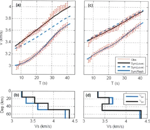
Figure 2-2. Rayleigh and Love phase velocity dispersion curves and shear wave speed models by the NA inversion at (25oN, 102oE) (a, b) and (27.5oN, 102oE) (c, d). (a) and (c): the red lines (with 1o error bars) are observed phase velocity dispersion curves for Love (top) and Rayleigh (bottom) wave, respectively. The standard error c is estimated from the seasonal variations of EGF (Yao et al., 2006). The black lines are the Love wave dispersion curves calculated from the VSH model in (b) and (d),
depth =10 km depth =25 km depth =35 kin 29 ... 29 29 8 2 2V 2 28 0 -h -2 -4 -e 24 - 27 27 ---100 101 102 103 104 100 101 102 103 104 100 101 102 103 104
Longitude (deg) Longitude (deg) Longftude (deg)
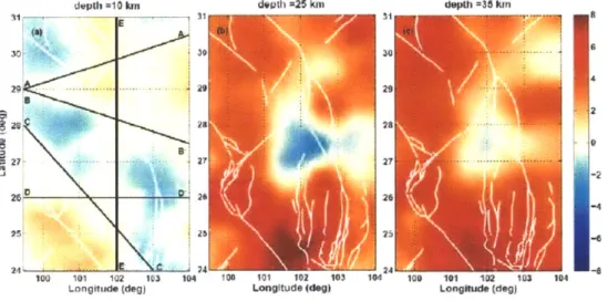
Figure 2-3. Radial anisotropy (y) defined as 2(VSH- Vsv)/(VsH+Vsv)*100 (%), at (a) 10 km, (b) 25 km and (c) 35 km depth. Red depicts VsH> Vsv (V > 0); blue indicates VSH
< Vsv (V < 0). White lines depict the major faults in our study area, and in (a) the thin
black lines with letters at each end indicate the location of vertical profiles in Figure 2-4.
I
El,
Ii:
0 0 100 200 300 400 600 600 700 Distance(km} (b) 0.~~0
a0 2 80 60--0 100 200 300 40 500 600 100 Distance(km)Figure 2-4. (a) The perturbation of shear wave velocity structure dln Vsv (%), with red (blue) depicting slow (fast) shear wave propagation. Topography is shown above each profile. The black thick lines in each profile (around 50 kin) depict the Moho discontinuity. The reference Vsv model in the curst is a 3 layered model with 3.3, 3.6, and 3.8 km/s in upper, middle and lower crust, which are inferred from the global Crust 2.0 model (http://mahi.ucsd.edu/Gabi/rem.html) by averaging Vs separately of the upper, middle, and lower crust for all locations with crustal thickness larger than 40 km. The reference Vsv in the upper mantle is the average of the whole study area. (b) Radial anisotropy, defined as 2(VsH- Vsv)/(VsH+Vsv)* 100 (%). Red represents VsH>
Vsv; and blue represents VSH < Vsv.
(a)
80
E
0
10 (a) 10 (b) 10 (c) 5 5+ 5 0 00 -5 -5 -5 -10
-10
-10 -_ -_-_--tO 0 10 -10 0 10 -10 0 10dInVsv(%) dInVsv(%) dInVsv (%)
Figure 2-5. Relationship between relative Vsv anomalies (dlnVsv) and radial anisotropy (qI) for (a) upper crust, (b) middle crust, and (c) lower crust. Each symbol represents a grid point on map. Colors represent different tectonic regions (as defined in Figure 2A-4): the Songpan-Ganze block (green), the Lhasa block (black), the Sichuan Basin (blue), the part of the Yangtze craton west of the Xianshuihe-Xiaojiang fault system (red), the part of the Yangtze block east of the Xianshuihe-Xiaojiang fault system (yellow), and the Youjiang block (cyan).
800
(a)(b) 600 .,400 2000
-600-400-200 0 200 400 600-600-400-200 0 200 400 600 t (s) t (s) 3 5 10 15 20 25 30 .35 40 5 10 15 20 25 30 35 40 T(s) T(s)Figure 2A-1. (a)-(b) Band-pass filtered (8-40s) EGFs for Rayleigh and Love waves, respectively. The red curves (multiplied by a factor of 5) are the EGFs used in (c)-(d) to extract phase velocity dispersion curves by an image transformation technique (Yao et al., 2005). (c)-(d) Phase velocity dispersion measurements from the EGFs for Rayleigh and Love wave, respectively. The white lines depict the extracted dispersion curves.
343 3.5 3,7 3.7 33.75 45 3.05 3.65 3.4 3. 37 3.255 3.5 3.3 375 36
$
1 3.45 355 26 23 43 75 3.2 375 3.354 135 345 3.4 3,5 364 345 335 S345 3.75 3,5 3.7 3.8 3A 3.653.65 3.35 V 1 33 4I-S 58 277 3.45 3 55 325 1004 01 102 13 104 3.5 100 101 102 503 104 5 1 00 101 102 10 104 33Longitude (dog) Longitude (dog) Longitude (dog)
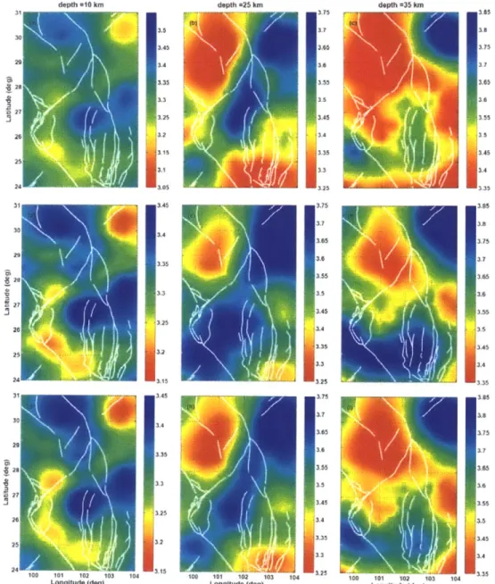
Figure 2A-2. Absolute wave speed (km/s) for Vsv (a)-(c), Vsh (d)-(f), and their
average (g)-(i) at at 10 km, 25 kn, and 35 km depth.
(a) CL50
0
E 0 50 0 60 0 100 20 0 300 400 600 Distancefkm) (b) 01-E A A 60 4 4 Cso-0 00 D 60 600 700 0 100 200 300 400 600 600 700 Distancelkm)Figure 2A-3. (a) Radial anisotropy when the Moho depth is 5 km larger than that from the receiver function analysis; (b) the change of radial anisotropy due to the Moho depth change (e.g. the difference between Figure 2A-3a and Figure 2A-4b).
31
*
*
* *
*
*
*
*
*
* * * * * * * * *30-
*
*
* *
*
*
*
*
* * * * * * *29-
*
*
*
*
*
*
*
* * * * * * *S28-
*
*
*
*
*
*
-7-2
27-
*
*
*
*
*
*
-J*
*
*
*
*
*
26-
* * * *
* * * *
*
*
*
*
*
*
*
*
25-
* * * *
* *
* *
*
*
*
*
*
*
*
*
24-
*
*
*
*
*
*
*
*
99
100
101
102
103
104
Longitude (deg)
Figure 2A-4. The six main tectonic regions for our study area. Each star represents a grid point in the inversion. Black curves are either major faults or unit boundaries (Figure 2-1). Each cross represents a grid point in our inversion. Green: Songpan-Ganze block; black: Lhasa block, dark blue: Sichuan Basin; red: the Yangtze craton west to the Xianshuihe-Xiaojiang fault system; yellow: Yangtze block east to the Xianshuihe-Xiaojiang fault system; and cyan: Youjiang block.
10 (a) 5
,-0
-5 -10, -10 0 10 dInVS (%) 10 5 0 -5 -10 -10 0 10 dInVsH (%) 10 5 0 -51 -10 -10 0 10 dInV (%)Figure 2A-5. Relationship between relative Vsv anomalies (dlnVsv) and radial anisotropy (y) for (a) upper crust; (b) middle crust and (c) lower crust. Each cross represents a grid point on map. Colors represent different tectonic regions defined in
Figure 2A-4.
(c)
I C,, 10 5 0 -5 10 5 0 -5 101(c) I 5 0 -5
-101
1
1
-IUL
I_____ IU I.
-10 0 10 -10 0 10 -10 0 10dInV, (%) dInV, (%) dInV, (%)
Figure 2A-6. Relationship between relative Vsv anomaly (dlnVsv) and Vsh anomaly (dlnVsh) for (a) upper crust; (b) middle crust and (c) lower crust. Each cross represents a grid point on map. Colors represent different tectonic regions defined in Figure 2A-4. (a) (b) *- --"I if a