Applying probabilistic rules to relational worlds

Applying Probabilistic Rules To Relational Worlds

by

Natalia Hernandez Gardiol

B.S. Computer Science, Michigan State University (1999)

Submitted to the

Department of Electrical Engineering and Computer Science

in partial fulfillment of the requirements for the degree of

Master of Science in Electrical Engineering and Computer Science

at the

MASSACHUSETTS INSTITUTE OF TECHNOLOGY

February 2003

©

Massachusetts Institute of Technology 2003. All rights reserved.

A uthor ...

Department of Electrical Engineering and Computer Science

November 25, 2002

C ertified by ...

Leslie Pack Kaelbling

Professor of Computer Science and Engineering

Thesis Supervisor

A ccepted by ...

...

Arthur C. Smith

Chairman, Department Committee on Graduate Students

MASSACHUSETTS INSTITUTE OF TECHNOLOGY

BARKER

Applying Probabilistic Rules To Relational Worlds

by

Natalia Hernandez Gardiol

Submitted to the Department of Electrical Engineering and Computer Science on November 25, 2002, in partial fulfillment of the

requirements for the degree of

Master of Science in Electrical Engineering and Computer Science

Abstract

Being able to represent and reason about the world as though it were composed of "objects" seems like a useful abstraction. The typical approach to representing a world composed of objects is to use a relational representation; however, other rep-resentations, such as deictic reprep-resentations, have also been studied. I am interested not only in an agent that is able to represent objects, but in one that is also able to act in order to achieve some task. This requires the ability to learn a plan of action. While value-based approaches to learning plans have been studied in the past, both with relational and deictic representations, I believe the shortcomings uncovered by those studies can be overcome by the use of a world model. Knowledge about how the world works has the advantage of being re-usable across specific tasks. In general, however, it is difficult to obtain a completely specified model about the world. This work attempts to characterize an approach to planning in a relational domain when the world model is represented as a potentially incomplete and/or redundant set of uncertain rules.

Thesis Supervisor: Leslie Pack Kaelbling

Acknowledgments

Without question, my thanks first and foremost go to my advisor, Leslie Pack Kael-bling. Without her keen insights, gentle advice, and unending patience, none of this work would have been possible. She is a constant and refreshing source of inspiration to me and to the people around her, and I am grateful to count myself among her students.

I thank my family for their unwavering support of my endeavors, both academic and otherwise, foolish and not. I owe to them the very basic notion that the natural world is an amazing thing about which to be curious. I thank my father especially, for demonstrating by his own example the discipline and the wonder that go with scientific inquiry. Los quiero mucho.

Here at MIT, I owe many people thanks for their support and patience. Sarah Finney has been an awesome collaborator and office-mate, and has taught me a great deal about how to ask questions. Luke Zettlemoyer sat with me on countless late nights discussing the intricacies of well-defined probability distributions. Terran Lane and Tim Oates generously shared their expertise with me and provided countless useful pointers. I thank Marilyn Pierce at the EECS headquarters for her amazing resource-fulness, patience, and personal attention, and for always keeping the students' best interests at heart.

This work was done within the Artificial Intelligence Lab at Massachusetts Institute of Technology. The research was sponsored by the Office of Naval Research contract N00014-00-1-0298, by the Nippon Telegraph & Telephone Corporation as part of the NTT/MIT Collaboration Agreement, and by a National Science Foundation Graduate Research Fellowship.

Contents

1 Introduction: Why Objects? 13

2 Background 16

2.1 Representational Approaches to Worlds with Objects . . . . 17

2.1.1 Relational Representations . . . . 17

2.1.2 Deictic Representations . . . . 18

2.2 Acting in Worlds with Objects: Value-Based Approaches . . . . 19

2.2.1 Relational Reinforcement Learning . . . . 19

2.2.2 Reinforcement Learning With Deictic Representations . . . . . 22

2.3 The Case for a World-Model . . . . 23

2.4 Reasoning with Probabilistic Knowledge . . . . 24

2.4.1 An Example: When Rules Overlap . . . . 25

2.5 Related Work in Probabilistic Logic . . . . 30

2.6 Related Work in Policy Learning for Blocks World . . . . 32

3 Reasoning System: Theoretical Basis 34 3.1 Probabilistic Inference with Incomplete Information . . . . 35

3.2 Using Probabilistic Relational Rules as a Generative Model . . . . 38

3.2.2 CLAUDIEN: Learning Probabilistic Rules . . . .4

4 Experiments 42 4.1 A Deterministic Blocks World . . . . 43

4.1.1 Acquiring the Set of Rules . . . . 46

4.1.2 Deterministic Planning Experiment . . . . 48

4.2 A Stochastic World with Complex Dynamics . . . . 50

4.2.1 Acquiring the Rules for the Stochastic Stacking Task ... 54

4.3 A Stochastic World with Simpler Dynamics . . . . 57

4.3.1 Acquiring the Rules for the Simpler Stochastic Stacking Task. 59 4.3.2 Planning Experiments . . . . 64

5 Conclusions 77 5.1 Combining Evidence . . . . 77

5.2 Learning and Planning with Rules . . . . 78

5.3 Future W ork . . . . 79

A Rules Learned by CLAUDIEN For the Deterministic Blocks World 84 40

List of Figures

2-1 How should we represent the blocks and the relationships between the blocks in this example blocks world? . . . . 16 2-2 The DBN induced by the move (c, d) action in the example world. . 26 2-3 The Noisy-OR combination rule . . . . 29

4-1 The RRL blocks world. The goal is to achieve on(a,b). . . . . 43 4-2 The deterministic world used by our system. The table is made of

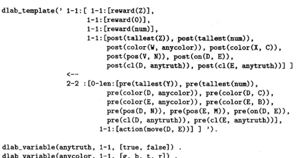
three table blocks, which may be subject to move attempts but are actually fixed. . . . . 44 4-3 The DLAB template for the deterministic blocks world. This template

describes rules for how actions, in conjunction with pre-conditions and/or a goal predicate, either produce a certain reward (either 1.0 or 0.0) or influence a single state predicate. In other words, it de-scribes a mapping from actions, state elements, and the goal predicate into a reward value of 1.0, a reward value of 0.0, or the post-state of a state element. The expression 1-1 before a set means that exactly one element of the set must appear in the rule; similarly, 3-3 means exactly three elements, 0-len means zero or more, etc. . . . . 47 4-4 Sample output from the planning experiment in the deterministic small

blocks world. . . . . 49 4-5 The large stochastic blocks world. The table is made up of fixed,

indistinguishable table blocks that may not be the subject of a move action. . . . . 51 4-6 The DLAB template, without background knowledge, used in the

4-7 The DLAB template, with background knowledge about next-to used in the complex block-stacking task. . . . . 55 4-8 The DLAB template used in the simpler stochastic block-stacking task.

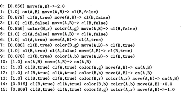
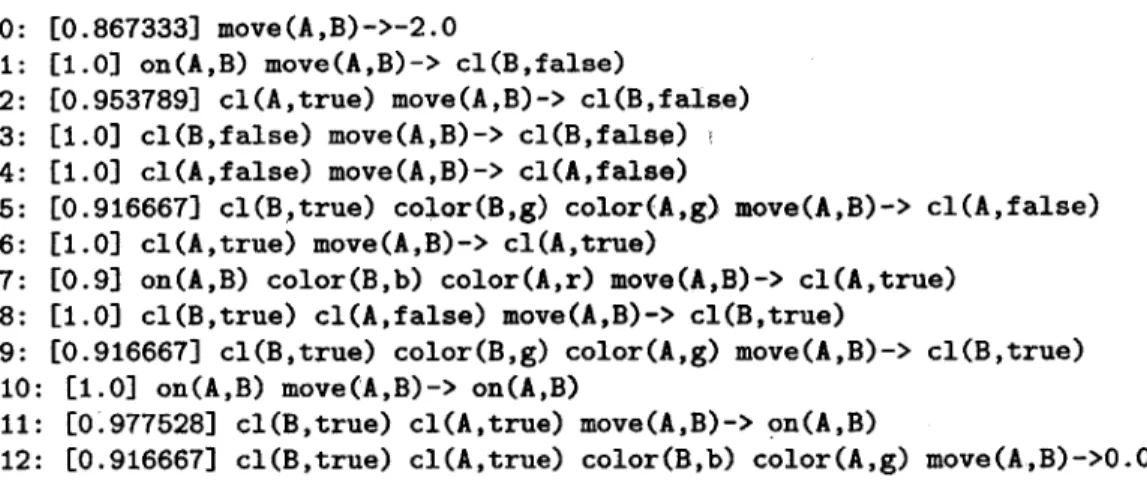
The same template was used in all stochasticity versions of the task. . 60 4-9 CLAUDIEN rules for the high-stochasticity version of the stacking task. 61 4-10 CLAUDIEN rules for the mid-stochasticity version of the stacking task. 61 4-11 CLAUDIEN rules for the low-stochasticity version of the stacking task. 62 4-12 Hand-coded rules, and corresponding probabilities, for the high-stochasticity

version of the stacking task. . . . . 63 4-13 Hand-coded rules, and corresponding probabilities, for the mid-stochasticity

version of the stacking task. . . . . 63 4-14 Hand-coded rules, and corresponding probabilities, for the low-stochasticity

version of the stacking task. . . . . 63 4-15 Plot of cumulative reward for the hand-coded rules in the one-step

planning experiments. . . . .. 65 4-16 Plot of cumulative reward for CLAUDIEN rules in the one-step planning

experim ent. . . . . 66 4-17 A small, example world for illustrating the DBN that results from

applying rules from the hand-coded set. . . . . 67 4-18 The DBN induced by applying-the hand-coded rules to the example

world in Figure 4-17 and the action move (n3, n1). It is sparse enough that a combination rule does not need to be applied. . . . . 69 4-19 Initial configuration of blocks in all the one-step planning experiments.

The configuration can also be seen schematically in Figure 4-5. Each block is represented by a pair of square brackets around the blocks' name and the first letter of the block's color (e.g., block n20 is red;

nOO is a table block). . . . . 70 4-20 Output from the CLAUDIEN rules in the low-stochasticity one-step task. 71 4-21 Output from the hand-coded rules in the low-stochasticity one-step task. 72 4-22 The smaller world used in the three-step planning experiments. . . . 73

4-23 Initial configuration of blocks in the three-step planning experiments. The configuration can also be seen schematically in Figure 4-22. . . . 73

4-24 Output from the CLAUDIEN rules in the low-stochasticity three-step task. 74 4-25 Output from the hand-coded rules in the low-stochasticity three-step

List of Tables

2.1 The conditional probability table for ontable (c). . . . . 27

Chapter 1

Introduction: Why Objects?

When human agents interact with their world, they often think of their environment as being composed of objects. These objects (chairs, desks, cars, pencils) are often described in terms of their properties as well as in terms of their relationship to the agent and to other objects.. Abstracting the world into a set of "objects" is useful not only for achieving a representation of what the agent perceives, but also for giving the agent a vocabulary for describing the goals and effects of its actions. Any "object" with the right set of properties can be the target of an action that knows how to handle objects with such properties, regardless of the specific object's identity. For example, if I have learned how to drink from a certain cup, then I should expect to be able to transfer my knowledge when presented with a different cup of approximately the same size and shape.

I want to build an artificial agent that can reason about objects in the world. Such an endeavor raises important questions about how objects in the world should be represented. When AI researchers first attempted to build systems that could han-dle a world with objects, a common approach was to use a first-order representation of the world and to learn properties about the world via inductive logic program-ming systems [43]. Traditional logic programprogram-ming systems, such as those based on

the language Prolog, are powerful, but they unfortunately require the world to be deterministic.

In contrast, for dealing with the world probabilistically, Bayesian networks [48] pro-vide an elegant framework. The difficulty with Bayes' nets, however, is that they are only able to manage propositional representations of state; that is, each node in the network stands for a particular attribute of the world and represents it as a ran-dom variable. The limitations of propositional representations are well-known: with propositional representations of the world, it is hard to reason about the relation-ships between concepts in general; all instances of the concept must be articulated and represented explicitly.

Consequently, there has been much recent interest in probabilistic extensions to first-order logic; that is, in ways to represent the world relationally (as in logic program-ming) and to reason about such representations in a manner that can handle uncer-tainty (as in Bayesian networks).

Probabilistic logic systems seek to answer queries about the world from probabilistic relational knowledge bases. This is important for an agent who needs to reason in a non-deterministic environment with objects. The concrete question I am interested in is how an agent with probabilistic relational knowledge might use its knowledge in order to act.

In general, there are two basic approaches for an agent to develop courses of action. The first, and simplest, is to directly learn a mapping from observations to actions without explicitly learning about how the world works. This approach, within a relational context, has been investigated by recent work on relational reinforcement learning [23, 21]. The second approach is to try to build up some kind of model of the world, and to use this model to predict the effects of actions.

If the agent has a model of the world, it can query this model and use the resulting predictions to make a plan. Traditionally, the complexity of the planning problem

scales badly with the size of the world representation. Kearns et al. give an algorithm for a sparse, approximate planning algorithm that works with a generative model of the world [31]. Unfortunately, a major difficulty is that acquiring a generative model of the world, in practice, is often intractable.

The system described in the following pages is an attempt to build an artificial agent that represents objects with a relational representation, builds a generative world model with probabilistic rules [15], and acts by sparse planning with the (potentially incomplete) model. The probabilistic rules that I consider are quite simple: they probabilistically map a first-order representation of a state situation and action to the first-order representation of the resulting state.

Chapter 2

Background

This chapter discusses some of the previous work that motivated this study. It ex-amines some previous approaches to representing objects, learning in worlds with objects, and reasoning probabilistically about objects.

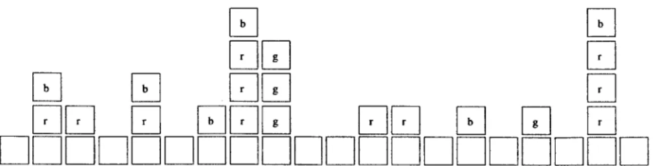
For the purposes of illustration, let us consider the following running example, seen in Figure 2-1. In this very small blocks world, there are three blocks; the blocks have certain properties and they are related to each other in certain ways. For example, block b is stacked on top of block a, and block c has nothing on top of it. Furthermore, we may have some general knowledge that it is only reasonable to try to move a block if it has no other blocks on top of it, and we might want to apply this knowledge to the block c. How to write down these properties, relations, and rules meaningfully is thus the subject of the following section.

JILL

Fb

Figure 2-1: How should we represent the blocks and the relationships between the blocks in this example blocks world?

2.1

Representational Approaches to Worlds with

Objects

When attempting to represent a world as being composed of objects, there are a number of ways to proceed. Below, we take a look at two approaches that have been considered in the past.

2.1.1

Relational Representations

The typical approach to describing objects and their relations is with a relational representation. For example, to describe the small blocks world shown in Figure 2-1, we could begin by writing down the following relational description:

on(b, a) nextto (c, a) ontable (c) ontable (a) clear (b) clear (c)

Relational representations have a great deal of expressive power. For example, we can articulate our rule for moving clear blocks onto other clear blocks in a way that is not specific to any individual object:

VC, B. clear(C) A clear(B) A move(C, B) -+ on(C, B)

This ability to generalize, to talk about any object satisfying particular properties, is what makes relational representations so appealing as a descriptive language. This is in contrast to propositional, or attribute vector, representations, which must refer to each individual object by name. Thus, when we want to represent a piece of knowledge, it must be repeated for every individual object in our universe:

clear(a), clear(b), move(a,b) -+on(a,b) clear(a), clear(c), move(a,c) -+on(a,c)

clear(b), clear(a), move(b,a) -+on(b,a)

clear(b), clear(c), move(b,c) -+on(b,c)

Even though relational representations are very convenient for describing situations succinctly, the question of how best to learn policies using a relational representa-tion remains an open problem. The most widely used reinforcement learning al-gorithms [55] all require propositional representations of state. Thus, even though relations are a compact and powerful way of articulating knowledge and policies, learning in such an expressive space remains difficult for standard methods.

2.1.2

Deictic Representations

Deictic representations hold the promise of potentially bridging the gap between purely propositional and purely relational representations. The term deictic

rep-resentation came into common use with the work of Agre and Chapman on the Pengi

domain [2]. It comes from the Greek word deiktikos, which means "to point": a

de-ictic expression is one that uses a conceptual marker to "point" at something in the

environment, for example, the-block-that-I'm-looking-at. An agent with an attentional marker on block c might describe the blocks world in Figure 2-1 like this:

ontable (the-block-that-I'm-looking-at) . clear (the-block-that-I'm-looking-at) .

has-block-nextto (the-block-that-I'm-looking-at) .

Deictic expressions themselves are propositional. Generalization is obtained by ac-tively moving the marker, or focus of attention, about. Depending on whether the agent is looking at block a, b or c, it will be able to use its knowledge about

the-block-that-I'm-looking-at in an adaptive way: the meaning of the attentional marker

At one extreme, essentially replicating a full propositional representation, the agent could have one marker for each object in its environment. In general, however, this is undesirable: the appeal of a deictic representation rests on the notion of a limited attentional resource that the agent actively directs to parts of the world relevant to its task. As a result, a deictic representation generally results in partial observability: the agent can directly observe part of its state space, but not all of it. So, while standard propositional reinforcement learning methods can be applied directly to a deictic representation, the partial observability is problematic for many learning algorithms [241.

2.2

Acting in Worlds with Objects: Value-Based

Approaches

This section describes recent work in value-based approaches to learning with rela-tional and deictic representations. As previously noted, a simple way to learn how to act is to learn a mapping from observations to actions without explicitly learning about how the world works. This approach is known as model-free reinforcement learning [55]. Recent work in reinforcement learning has focused on investigating rep-resentations that have generalization properties while remaining amenable to model-free approaches [23, 21]. The reason for investigating alternative representations is to avoid the limitations of propositional representations: because propositional repre-sentations are grounded in terms of specific objects, as soon as the world or the task changes slightly, the agent is forced to re-learn its strategy from scratch.

2.2.1

Relational Reinforcement Learning

The work of Dzeroski, De Raedt, and Driessens [19] on relational reinforcement learn-ing uses a tree-based function approximator to approximate the Q-values in a

rela-tional blocks world.

The relational reinforcement learning (RRL) algorithm is a logic-based regression algorithm that assumes a deterministic, Markovian domain. The planning task in-cludes:

" A set of states. The states are described in terms of a list of ground facts. " A set of actions.

" A set of pre-conditions on the action specifying whether an action is applicable in a particular state.

" A goal predicate that indicates whether the specified goal is satisfied by the current state.

" A starting state.

In its basic form, the algorithm is a batch algorithm that operates on a group training episodes. An episode is a sequence of states and actions from the initial state to the state in which the goal was satisfied. There is also an incremental version of the algorithm, described by Driessens [19]. Here is the basic RRL algorithm:

1. Generate an episode; that is, a sequence of examples where each example con-sists of a state, and action, and the immediate reward.

2. Compute Q-values [56] for each example in the episode, working backwards from the end of the episode. The last example in an episode (i.e., the one in which the goal is achieved) is defined to have a Q-value of zero. The Q-values are computed with the following rule, where the Q-value for example j is being computed from example j + 1:

3. Present the episode, labeled with the computed Q-values, to the TILDE-RT [15]

algorithm. Given labeled data, TILDE-RT induces logical decision trees. In the case of RRL, the decision trees would specify which predicate symbols in the state description are sufficient to predict the Q-value for that state.

RRL assumes a deterministic domain. It stores all the training examples and re-generates the decision tree (also called regression tree, or Q-tree) from scratch after each episode.

In the longer version of the paper ([21, 22]), Dzeroski et al. augment the batch RRL algorithm by learning what are called P-trees in addition to the Q-trees. The basic problem is that value functions implicitly encode the "distance to the goal"; in the case of blocks world, this limits the applicability of the learned value function when moving to a domain with a different number of blocks. Thus, given a Q-tree, a P-tree can be constructed that simply lists the optimal action for a state (i.e., the action with the highest Q-value) rather than storing explicitly the Q-value for each action. Dzeroski et al. find that policies taken from P-trees generalize best when the Q-tree is initially learned in small domains; then, the P-tree usually generalizes well to domains with a different number of blocks.

Additionally, the authors noted that for more complicated tasks (namely, achiev-ing on(a,b)) learnachiev-ing was hindered without a way to represent some intermediate concepts, such as clear (a), or number-of-blocks-above (a, N). They note that be-ing able to express such concepts seems key for the success of policy learnbe-ing. The apparently "delicate" nature of these intermediate concepts, their inherent domain dependence, argues strongly for a system that can define such concepts for itself. The incremental version [19] uses an incremental tree algorithm based on the G algorithm of Chapman and Kaelbling [12] to build the regression trees as data arrives. Apart from the difficulties inherent to growing a decision tree incrementally,1 the main

'Namely, having to commit to a branch potentially prematurely. See the discussions in [19, 23]

challenge presented by the relational formulation is in what refinement operator to use for proposing new tree branches. In contrast to the propositional case, where a query branch is refined2 by simply proposing to extend the branch by a feature not already tested higher in the tree, in the relational case there are any number of ways to refine a query. Proposing and tracking the candidate queries is a difficult task, and

it is clearly an important and open problem.

2.2.2

Reinforcement Learning With Deictic Representations

Deictic representation is a way of achieving generalization that appears to avoid some of the difficulties presented by relational representations. Because of their propo-sitional nature, deictic representations can be used directly in standard reinforce-ment learning approaches. However, the consequence of having limited attentional resources is that the world now becomes partially observable; that is to say, it is described by a partially observable Markov decision process (POMDP) [49].

When the agent is unable to determine the state of the world with its immediate observation, the agent must refer to information outside of the immediate perception in order to disambiguate its situation in the world. The typical approaches are to either add a fixed window of short-term history [42, 41] or to try to build a gener-ative model of the world for state estimation [30, 36]. Reinforcement learning with the history-based approach is simple and appealing, but there can be some severe consequences stemming from this approach [23].

Finney et al.[24] showed that using short-term history with deictic representations can be especially problematic. They studied a blocks-world task in which the agent was given one attentional marker and one "place-holding" marker. The environment consisted of a small number of blocks in which the task was to uncover a green block and pick it up. The agent was given actions to pick up blocks, put down blocks,

2

and move the attentional marker. At each time step, the agent received perceptual information (color, location, etc) about the block on which the attentional marker was focused. Neuro-dynamic programming [7] and a tree-based function approximator [12] were used to map short history sequences (i.e., action and observation pairs) to values. This approach generates a dilemma. Because the history the agent needs in order to disambiguate its immediate observations depends on the actions it has executed, until it has learned an effective policy, its history is usually uninformative. It is even possible, with a sufficiently poor action choices, to actively push disambiguating in-formation off the end of the history window. Alarmingly, this can happen regardless of the length of the history window. This difficulty was also noticed by McCallum in his work on reinforcement learning with deictic representations [41]. McCallum was able to get around this problem by guiding the agent's initial exploration. Neverthe-less, the question of how best to use your history when you do not yet know what to do is a very fundamental bootstrapping problem with no obvious solution.

2.3

The Case for a World-Model

The challenges presented by model-free, value-based reinforcement learning, with both relational and deictic representations, argue compellingly for a model with which to estimate the state of the world.

When the agent has a generative model of the world, it can query this model to decide its next action. The idea of an agent with some knowledge of world dynamics is appealing because then the agent is able to hypothesize the effects of its actions, rather than simply reacting to its immediate observation or to windows of history. A model allows the agent to plan its actions based on the current state of the world, rather than having to compute a whole policy in advance. However, the complexity of generating a plan typically scales badly with the size of the world representation and the number of possible actions. To address the scaling problem, Kearns et al.

give an algorithm for a sparse, approximate planning algorithm that works with a generative model of the world [31].

A major difficulty is that learning a full generative model of the world is often hope-lessly intractable. It is often unreasonable to expect the agent to come up with a full model of the world before it can begin to act. Intuitively, it seems likely that the agent should be able to begin to apply whatever knowledge it has as soon as it is acquired.

This is the major thrust of this work: exploring what it means to plan with a world model that is by necessity incomplete and perhaps inconveniently redundant.

2.4

Reasoning with Probabilistic Knowledge

When an agent's knowledge about the world is incomplete, the theory of probability becomes extremely useful. Probability theory gives a powerful way to address the uncertainty brought on by missing information. The converse of not having enough information is having pieces of evidence that overlap. How to reconcile bits of knowl-edge when their predictions about the next state of the world overlap is another important issue that requires probability theory.

The approach described in this work adopts the spirit of direct inference: it takes gen-eral statistical information and uses it to draw conclusions about specific individuals, or situations. Much of the work in direct inference depends on the notion of finding a suitable reference class [50] from which to draw -conclusions. That is to say, given a number of competing pieces of evidence, which piece of evidence is the correct one to apply in the current specific situation? This is a deep problem, addressed in detail by Bacchus et al. [3]. My approach is to adopt some assumptions about the evidence, and then to combine the evidence using standard probability combination rules that make those same assumptions. Combining the evidence in this way is appealing for

its simplicity and speed, and it should lead to reasonable performance within the constraints of the assumptions.

2.4.1

An Example: When Rules Overlap

Let us see what this means in the context of our example. Say we have two first-order rules as follows.

1. With probability 0.1: move(A, B) clear(A) -* ontable(A) 2. With probability 0.3: move(A, B) slippery(B) - ontable(A)

These rules express the knowledge that

1. In general, moving any block A incurs some small probability of dropping the block onto the table.

2. Moving any block A onto a slippery block can result in block A falling on the table.

If we are considering a move (c,b) action, both of these rules apply. What probability should we assign to ontable (c)? That is, how should we compute

P(ontable(c)

I

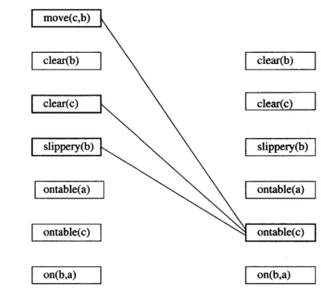
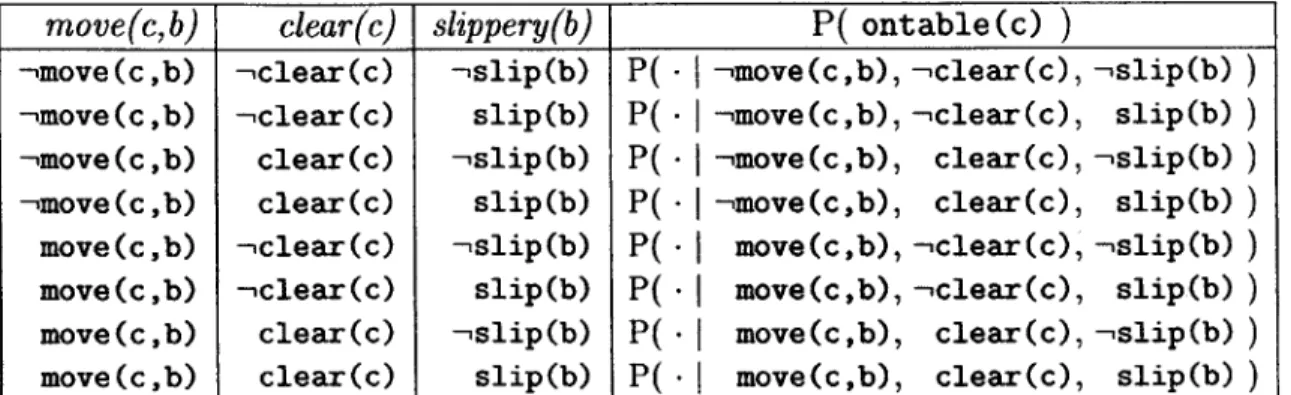
Let us describe the probability distribution over next states by the dynamic Bayesian network (DBN) shown in Figure 2-2. To be fully specified, the conditional probability table in the DBN for ontable (c) needs to have entries for all of its rows.

The basic problem is that the conditional probability tables (CPTs) associated with the logical rules do not define a complete probability distribution in combination. That is, the rules only give us the following information:

move(c,b) clear(b) clear(b) clear(c) clear(c) slippery(b) slippery(b)] ontable(a): _ontable(a): ontable(c) ontable(c) on(b,a) on(b,a)

Figure 2-2: The DBN induced by the move (c, d) action in the example world.

1. P( ontable(c)

I

J

To simplify the notation, let us refer to the random variable ontable(c) as 0; move(c, b) as M; slippery(b) as S; and clear(c) as C. If ontable(c) ranges over ontable(c) and -ontable(c), then we abbreviate it by saying 0 ranges over o and -,o. And so on for the other random variables.

One way to compute the probability value we need, i.e., P(o I m, s, c) is to adopt a maximum entropy approach, and to search for the least committed joint probability distribution P(0, M, S, C) that satisfies the three constraints:

a, = P(o I m, c)

= P(o, m, c)/P(m, c)

= EP(So,m,c)/EP(SOm,c)

move(c,b) clear(c) slippery(b) P( ontable(c) )

,move (c,b) -,clear (c) -slip(b) P( -- move(c,b), -,clear(c), -,slip(b) )

-move (c ,b) -,clear (c) slip(b) P( - -move(c,b), -,clear(c), slip(b)

-move (c,b) clear(c) -,slip(b) P( - -move(c,b), clear(c), -,slip(b) )

-move(c,b) clear(c) slip(b) P( - -move(c,b), clear(c), slip(b)

move(c,b) -clear (c) -,slip(b) P( -I move(c,b), -clear(c), -,slip(b) )

move(c,b) -,clear (c) slip(b) P( - move(c,b), -clear(c), slip(b) )

move (c ,b) clear(c) -slip (b) P( -I move(c,b), clear(c), -,slip(b) )

move(c,b) clear(c) slip(b) P( -

f

Table 2.1: The conditional probability table for ontable (c).

a₁

Z

Z

Having found such a distribution, we could solve for P(o I m, s, c) by setting it equal to

P(o, m, s, c)

P(o j m, s, c) - mSC) .P(O

EO P(0, M, S, C)

However, the maximum entropy approach requires a maximization over 24 unknowns: P(o, m, s, c), P(o, m) s, - c), P(o, m,

-s,

(2.1)

(2.2)

But this calculation seems like overkill: all we really want is to predict the value of P(ontable(c)) for the current situation; that is, the situation in which O=o, M=m, S=s, and C=c. Furthermore, it has been observed that maximum entropy approaches exhibit counter-intuitive results when applied to causal or temporal knowledge bases [28, 48]. If we assume we have some background knowledge, there is no need to be as non-committal as maximum entropy prescribes. In fact, a useful way to articulate domain knowledge when it comes to combining rules with under-specified CPTs is through a combination rule.

A combination rule is a way to go from a set of CPTs, P(alaii, . , aini)

P(aja₂, ,a2n2

P(alami, ,amnm)

to a single combined CPT,

P(alai, an

where {ai, -- -, an} C UTM{aj, - ai}.

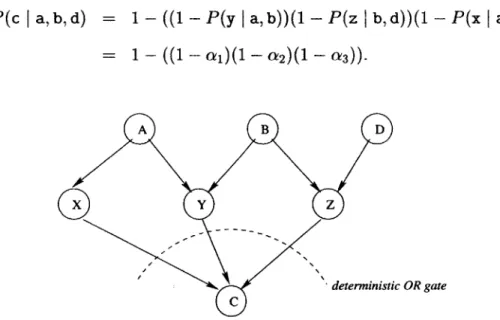
In general, a combination rule is a design choice. In this work, I used the Noisy-OR combination rule and the Dempster combination rule [53].

The Noisy-OR rule is a simple way of describing the probability for an effect given the presence or absence of its causes. It makes a very strong assumption that each causal process is independent of the other causes: the presence of any single cause is sufficient to cause the effect, and absence of the effect is due to the independent

"failure" of all causes. Consider an example with four random variables, A, B, C, D (respectively ranging over a and -,a, b and -,b, etc.) shown in Figure 2-3. Say we want to compute P(c I a, b, d), and that we know:

P(c a, b) P(c d, b) P(c

I

-The model in Figure 2-3 describes the idea that the random variables A, B, D each influence intermediate variables, X, Y, Z: conceptually, the probability of X being "on" is a3, the probability of Y being "on" is a1, and the probability Z being "on"

is a2. These intermediate variables in turn influence C. Noisy-OR asserts that if

any one of X,Y, or Z is "on," that is sufficient to turn C "on" .3 Noisy-OR asserts that the probability of C being "off" is equal to the probability of X,Y, and Z all independently failing to be "on." Therefore, according to Noisy-OR:

P(c a,b,d) = 1- ((1 -P(y l a,b))(1 - P(z

i

I

= 1 -((1 -a1)(1 -a2)(1 - a3)).

A B D

x Y Z

deterministic OR gate

C

Figure 2-3: The Noisy-OR combination rule.

The Dempster combination rule assumes that the competing rules axe essentially independent; that is, it asserts the sets of situations described by each rule overlap only on the current query situation. Each probabilistic rule represents the proportion of the predicted effect in its corresponding set. It has the underlying notion that the proportions of evidence are, in some sense, cumulative. Thus, if a is the probability

3_{1n other words, "turning C on"}

that rule i gives to P(c), then the Dempster rule states:

P(c

I

Both combination rules make fairly strong independence assumptions about the com-peting causes. The Dempster rule assumes an additive quality about the evidence (which seems appropriate in the case where we search for high-probability rules about action effects), but the Noisy-OR rule is simpler to compute. That being said, there are any number of ways to go from a set of rules to a single probability (e.g., choos-ing the most specific rule, computchoos-ing a consistent maximum entropy distribution, etc.); in general, combination rules are ad hoc and assume particular characteristics about the domain. Combining evidence in the general case is truly hard; the reader is again referred to Bacchus et al. [3] for the analysis and discussion of a more general approach.

2.5

Related Work in Probabilistic Logic

Bayesian networks are well known for their ability to manage probabilities associ-ated with world knowledge, but they generally handle only propositional knowledge. Extending relational, or first-order, representations so that they can be managed probabilistically is therefore an important area of study. Ground has been broken in this area by Ngo and Haddawy [45], Koller and Pfeffer [35], Jaeger [29], Russell and Pasula [47], Lukasiewicz [37]. Kersting and De Raedt provide a nice survey of these approaches [32].

The probabilistic relational models (PRMs) of Koller and Pfeffer, inspiring the subse-quent work by Pasula and Russell, bring in elements from object-oriented databases and couch the qualitative state information in terms of the entity/relationship model from that literature, instead of in terms of logical clauses. The PRM framework

pro-vides a mechanism for combining CPTs in the form of "aggregate functions," which again are provided by the designer. In contrast, the work of Lukasiewicz on proba-bilistic logic programming gets around the question of combination rules by specifying that the CPTs should be combined in a way that produces the combined probability distribution with maximum entropy.

Kersting and De Raedt give an interesting synthesis of these first three approaches and provide a unifying framework, called "Bayesian Logic Programs." A Bayesian Logic program consists of two parts: a set of logical clauses qualitatively describing the world, and a set of conditional probability tables (CPTs), plus a combination rule, encoding quantitative information over those clauses. The way logical queries are answered in this framework is by building up a tree structure that represents the logical proof of the query; the probabilistic computations are propagated along the tree according to the specified combination rule.

I adopt a rule-based approach, rather than the Bayesian Logic or PRM approach, because of the need to express temporal effects of actions. PRMs provide a rich syntax for expressing uncertainty about complex structures; however, the structure I need to capture is dynamic in nature. It is not immediately clear if the extension from static PRMs to dynamic PRMs is as straightforward as the DBN case. More fundamentally, PRMs require a fully described probability distribution. That is, that every row in the conditional probability tables for every slot must be filled in. For the purposes of modeling the immediate effect of a chosen action, however, such detail is hard to come by and may not be actually needed (see discussion above). For these reasons, the simpler approach of probabilistic rules in conjunction with a combination rule seems more appropriate for modeling the effects of actions in a relational setting.

2.6

Related Work in Policy Learning for Blocks

World

Apart from the traditional planning work in blocks worlds, there is an interesting line of work in directly learning policies for worlds not represented in a first-order language.

Martin and Geffner [39], and Yoon et al. [57] use concept languages to find generalized policies for blocks world. They build on the work of Khardon [33], who first learned generalized policies for blocks world within a first-order context. The basic approach is to start with a set of solved examples (usually obtained by solving a small instance of the target domain with a standard planning algorithm, called the teacher). Then, a search through the language space is conducted to find rules which best cover the examples. Khardon's approach is to enumerate all the rules possible within the language, and then to use a version of Rivest's algorithm for learning decision lists [52] to greedily select out the "best" rule, one by one, until all the training examples are covered. The learned policy, then, is articulated in the form of a decision list: the current state is compared to each condition in the list, and the action specified by the first matching rule is taken. The resulting policy is able to solve instances of the problem that the teacher is unable to solve.

Martin and Geffner expand on Khardon's work by moving from a first-order language to a concept language [9, 10, 44]. They notice that the success of Khardon's approach hinges on some intermediate support predicates that had to be coded into the repre-sentation by hand. For example, Khardon includes a predicate that indicates whether a block is a member of the set of blocks that are inplace; that is, blocks that have been correctly placed so far, given the goal specification. They reason that the ability of a concept language to express knowledge of sets or classes of objects would make

it possible to learn concepts like inplace automatically.

search to find the "best" rules, rather exhaustively enumerating of all the rules in the language space first. Second, they use bagging [11] to assemble a set of of decision-list policies (each trained on a subset of the training examples). The ensemble then chooses the action at each time step by voting.

Baum [5, 6] uses evolutionary methods to learn policies for a propositional blocks world. Each individual that is evolved represents a condition-action pair. Then, each individual learns how much its action is worth, when its condition holds, using temporal difference learning. Baum calls this the individual's bid. When it comes time to choose an action, the applicable individuals bid for the privilege of acting; the individual with the highest bid will get to execute its action. The learning of bids is described as an economic system, with strong pressure on each individual to learn an accurate value for itself. Individuals of low worth are eliminated from the pool, and evolutionary methods are applied to the individuals that succeed. What's interesting about this approach is that the learning, of both the rule conditions, and of the action values, is completely autonomous.

The above work represents successful instances of planning in blocks world: these systems aim to find policy lists that prescribe an action given certain conditions. The approach taken here is different, however. I am interested in modeling the dynamics of a relational domain (rather learning a policy ahead of time). Accordingly, I will pursue the approach of using first-order rules to probabilistically describe the effects of actions.

Chapter 3

Reasoning System: Theoretical

Basis

We want to represent the world as a set of first-order relations over symbolic objects in order to learn a definition of the world's dynamics that is independent of the specific domain. The first-order rules in our system describe knowledge in the abstract, like a skeleton in the PRM sense [26, 25]. To use abstract knowledge for reasoning about concrete world situations, we take the approach of direct inference [50]. That is to say, we ground the rules' symbols by resolving the rules against the current state, and then we make conclusions about the world directly from the grounded rules. In the rest of this document, the use of italic font in a rule denotes abstract, world-independent knowledge, and fixed-width font denotes ground elements.

Let us define a relational, or first-order, MDP as follows. The definition is based on the PSTRIPS MDP as defined by Yoon et al. [57].

A relational MDP has a finite set of states and actions. The actions change the state of the world stochastically, according to the probability distribution P(s, a, s'). There is a distribution R(s, a) that associates each state and action pair stochastically with the immediate real-valued reward.

" States: The set of states is defined in terms of a finite set S of predicate symbols, representing the properties (if unary) and relations (if n-ary) among the domain objects. The set of domain objects is finite, as well.

" Actions: The set of actions is defined in terms of action symbols, which are analogous to the predicate symbols. The total number of actions depends on

the cardinality (that is, the number of arguments) of each action and the number of objects in the world.

" Probability and reward distributions: For each action, we construct a dynamic Bayesian network [16] that defines the probability distribution over next states and rewards.

3.1

Probabilistic Inference with Incomplete

Infor-mation

Given a set of rules about how the agent's actions affect the world, we would like to turn them into a usable world model. We want to pull out those rules that apply to the current situation and use them to generate, with appropriate likelihood, the expected next situation.

To continue with our example, a first-order MDP description of the world in Figure 2-1 would be as follows.

e Set of action symbols:

Arity Description Example

move binary Move a block onto the top of another. move(a,b)

e The probability distribution over next states, P, and over next reward, R, can be represented with a dynamic Bayesian network (DBN) for each action. Say we are considering the the move (a, b) action that the applicable rules are

1. With probability 0.1: move(A, B) clear(A) -+ ontable(A), and 2. With probability 0.3: move(A, B) slippery(B) -+ ontable(A)

It should be immediately clear that the conditional probability tables on each arc of the DBN are incomplete, as we described in the previous chapter. What should the distribution be over clear(a), on(a,b)? What should it be for the state elements with no rules? What should the value of the reward be?

We need a precise definition of what to do when:

1. More than one rule influences a subsequent state element, or 2. No rule influences a subsequent state element.

Arity Description Example

clear unary Whether a block is clear. clear(a) slippery unary Whether a block is slippery. slippery(a) ontable unary Whether a block is on the table. ontable (a) on binary Whether a block is on top of another. on(a,b) nextto binary Whether a block is beside another. nextto(a,b)

Both of these problems result from incomplete information. The solution for the first item lies in finding a distribution that is consistent with the information available. The solution to the second problem additionally requires making some assumptions about the nature of the domain.

An appropriate way to express such domain knowledge is through the use of a com-bination rule, as described in the previous chapter. The system assumes a relatively static world and that the state elements may take on any number of discrete values (up until now, our examples have been with binary-valued state elements). Thus, we adopt the following approach:

1. If there is no information about a particular dimension, the value will not change from one state to the next, except for some small "leak" probability with which the dimension might take on a value randomly. In the experiments that follow, the "leak" probability was 0.01.

2. If there is more than one rule with influence on a particular value for a state element, their probabilities are combined via a combination rule. This yields the probability of generating that value.

Now, here comes a crucial assumption. For a given state element, the system takes all of the pieces of evidence for a value and normalizes their probabilities. This means, for example, that if the applicable rules only mention one particular value, then after normalizing that value gets a probability of one. It a value is not mentioned by any rule, it gets a probability of zero.' Knowledge about how the rules are acquired is important here. For example, if we do not have a rule about a particular situation, and we can safely assume that a lack of a rule implies a lack of meaningful

regularity-'Perhaps a better alternative would have been to divide the remaining mass evenly among the remaining possible values; however, this puts one into the awkward position of having to articulate all the possible (and potentially never-achieved) values of a perceptual dimension. The system does allow, however, for the user to explicitly supply an "alternative" value - if such a value is available,

it can be generated with the leak probability of E, and the rest of the probability mass is normalized

then, in this case, it is probably fine not to consider values that do not appear explicitly in any of the rules for the situation in question. The dimension's next value, then, is generated by choosing a value according to the normalized probability distribution.

3.2

Using Probabilistic Relational Rules as a

Gen-erative Model

The relational generative model consists of a set of relational rules, represented as Horn clauses, called the rule-base. Optionally, it can contain a set of background facts, called the bgKB. When queried with a proposed action and a current state, the model outputs a sampled next state and the estimated immediate reward.

Here are the steps for generating the next state and reward:

1. Turn the action and current observation into a set of relational predicates. Call it the stateKB. If background knowledge exists, concatenate the bgKB to the stateKB to make a new, larger, stateKB.

2. Compare each rule in the rule-base against each predicate in the stateKB. Given a particular rule, if there is a way to bind its variables such that the rule's antecedents and action unify against the stateKB (i.e., if the rule can be said to apply to the current state), then:

(a) Add the rule, along with all the legal bindings, to the list of matching rules. (b) "Instantiate" the rule's consequent (i.e., right-hand side) according to each

possible binding. This generates a list of one or more instantiated con-sequences, where each instantiation represents evidence for a particular value for a state element. Associate each instantiation with the probabil-ity recorded for the rule.

3. For each state dimension, look through the list of matching rules for instantia-tions that give evidence for a value for this dimension. Collect the evidence for each value.

(a) If there is more than one piece of evidence for a value, then compute a probability for the value according to the combination rule.

(b) Normalize the probabilities associated with each value, so that the proba-bilities for each value sum to one.

(c) Generate a sampled next value for this state dimension according to the normalized probabilities.

4. For the reward, look through the list of matching rules for instantiations that give evidence for a reward value. Compute a weighted average across all the reward values.

3.2.1

The Sparse-Sampling Planner

The generative world models produced by the above rules are by necessity stochastic and incomplete; whatever planning algorithm is used must take this uncertainty into consideration. To this end, I implemented the sparse-sampling algorithm by Kearns, Mansour and Ng [31]. In contrast to traditional algorithms where the search examines all the states generated by all the actions, the sparse sampler uses a look-ahead tree to estimate the value of each action by sampling randomly among the next-states generated by the action. As with all planning algorithms, this algorithm has the disadvantage of scaling exponentially with the horizon; but, the sparse-sampling trades that off with the advantage of not having to grow with the size of the state space.

The algorithm's look-ahead tree has two main parameters: the horizon and the width. These parameters depend on the discount factor, the amount of maximum reward, and the desired approximation to optimality. Kearns et al. provide guaranteed bounds on

the required horizon and width to achieve the desired degree of accuracy. However, with a discount factor of 0.9, a maximum reward of 1.0, and a tolerance of 0.1, for example, the computed parameters are a horizon of 80 and a width of 2, 147,483,647. Such numbers are, unfortunately, not very practical. As a result, the authors offer a number of suggestions for the use of the algorithm in practice, such as iterative deepening, or standard pruning methods.

However, there is unavoidable computational explosion with the depth of the horizon. It becomes especially acute if the action set size is anything but trivial (i.e., less than 5 actions). Although it is true that the number of state samples required is bounded (by the width parameter; in other words, the number of states that are sampled does not grow with the size of the state space) in order to estimate each sample's value, we need to find the maximum Q-value for the sampled state. This involves trying out each action at each level of depth in the tree, resulting in a potentially huge fan-out at each level. While it is possible to try to keep the action set small, it is not clear what solutions are available if one genuinely has a large action set, however. In the case of blocks world, for example, a large number of blocks produces a huge number of move(A, B)-type actions; in fact, the number of actions grows quadratically with the number of blocks.

This system does not try to prune the action explosion at all, although this is clearly desirable. The width and depth are set to rather arbitrary small values; the idea is to allow some degree of robustness, while at the same time permitting manageable computation time.

3.2.2 CLAUDIEN: Learning Probabilistic Rules

The CLAUDIEN system is an inductive logic engine for "clausal discovery" [15, 14]. It discovers clausal regularities in unclassified relational data. CLAUDIEN operates by a general-to-specific search to find a hypothesis set of clauses that best characterize the

presented data. It assumes a closed world - predicates that are not explicitly listed as true are assumed to be false.

CLAUDIEN is a batch system that takes as input a set of training examples. It then "data mines" the training set for the most compact set of Horn-clause rules that entail the examples in the set. Any variables in the rules are implicitly universally quantified.

The search space is specified by the user in terms of declarative bias [17]. This bias, which describes the set of clauses that may appear in a hypothesis, is provided according to the rules in a formalism called DLAB. A DLAB grammar is a set of templates that tells CLAUDIEN what the characterizing regularities should look like. Getting this bias right is absolutely crucial: CLAUDIEN will not find anything outside of the described search space; but, a space that is too large results in an intolerably long search.

The main user-definable parameters are called accuracy and coverage. Coverage spec-ifies the minimum number of examples a potential rule must "explain" in order to be considered. Accuracy specifies the minimum proportion of the examples explained (i.e., examples in which the pre-conditions apply) by the rule, to which the rule's post-conditions must also apply. The choice of parameters was somewhat arbitrary; I wanted to find rules that explained a non-trivial number of cases, and that explained them with high probability. Thus, coverage was set to 10 and accuracy was set to 0.9.

Because of its data-mining nature, CLAUDIEN seemed like the right approach for uncovering regularities about how actions affect the world. Other inductive logic programming systems, such as FOIL, are designed for classification problems, with positive and negative examples. Learning about the effects of actions seems more easily expressed as a data-mining problem than as a classification problem.

Chapter 4

Experiments

There were two main parts to the experiments. The first part examines how well a model-based system could perform compared to a value-based reinforcement learning system in a relational domain. To that end, I implemented a small, deterministic blocks world (see Figure 4-2) in order to draw some comparisons to the RRL system. The second part moves into a stochastic domain to truly exploit the probabilistic nature of the rules.

The main learning problem is in the acquisition of a set of first-order rules about the world dynamics-the world model. Resolving such a set of rules against the current observation and proposed action produces a set of grounded rules; these ground rules can be used to partially specify a DBN describing the effect of the action. We call this step applying the model to the world. At each step, to decide its next action, the agent invokes the planner. The planner applies the model to the current state, and successively to each predicted next-state, to ultimately produce an estimated Q-value for each action. The action chosen is the one with the highest estimated value; if there is more than one action at the highest Q-value, the planner chooses randomly among them.

4.1

A Deterministic Blocks World

In order to be able to draw comparisons to the RRL results, I used a blocks-world setup as close as possible to the one in the RRL experiments [21], although there are some slight differences which will be duly noted. The task in the RRL experiment to

move block a onto block b. The domain is shown in Figure 4-1.

a]

Figure 4-1: The RRL blocks world. The goal is to achieve on(a,b).

For comparison, here is the description of the blocks world used by the RRL system:

* State predicates:

Arity Description Example

clear unary Whether a block is clear. clear (a) on binary Whether a block is on top of another on (a, b)

block or on top of the table. on(a,table) goal unary Specifies the goal predicate. goal(on(a,b))

e Action symbol:

Arity Description Example

move binary Move a block onto the top of another. move (a, b) Can only be executed if the

* Action preconditions: allow move(A,B) if A : B and

A E{r,b,g}, B E {r,b,g,table}

* Reward: The reward is 1.0 0.0 otherwise.

if block a is successfully moved onto block b, and

Figure 4-2: The deterministic world used by our system. The table is made of three table blocks, which may be subject to move attempts but are actually fixed.

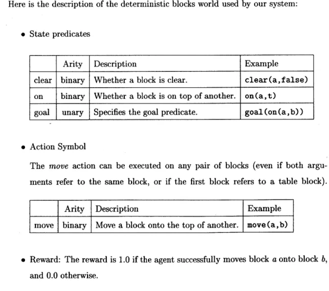
Here is the description of the deterministic blocks world used by our system:

" State predicates

Arity Description Example

clear binary Whether a block is clear. clear(afalse) on binary Whether a block is on top of another. on(at)

goal unary Specifies the goal predicate. goal(ona,b))

" Action Symbol

The move action can be executed on any pair of blocks (even if both argu-ments refer to the same block, or if the first block refers to a table block).

Arity Description Example

move binary Move a block onto the top of another. move (a,b)

" Reward: The reward is 1.0 if the agent successfully moves block a onto block b, and 0.0 otherwise.

As in the RRL setup, the agent observes the properties of the three colored blocks, as well as the goal. This yields an observation space of size 513. One difference from the RRL system is that the above observation vector includes clear (b, f alse), whereas in the RRL system if b were not clear then clear (b) would simply be absent. An example observation vector for our deterministic planner looks like this:

on(c,b). clear(c,true). on(b, a). clear(b,false). on(a, t) clear(a,false). goal(on(a,b)).

The reason for predicates like clear (c, f alse) and not like on(c, a, f alse) is that our system does not infer that the absence of clear (c) implies that clear (c) is false; in other words, it does not make a closed world assumption. Because pre-conditions are not built into the action specifications, knowing explicitly that a block is not clear is needed for estimating the success of a possible move action.

As in the RRL setup, the agent's action space consists of a move action with two arguments: the first argument indicates which block is to be moved, and the second argument indicates the block onto which the first one is to be moved. The action only succeeds if both of the blocks in question are clear; that is, they have no other blocks on top of them. Because the agent can consider all combinations of the six blocks as arguments to the move action, this yields 36 actions. In contrast, the RRL system only allows move(A,B) where A A B and A E {a,b,c}, B E {a,b,c,t}, a total of nine actions. Additionally, the table is three blocks wide, and the agent may attempt to pick up the blocks that make up the table. In the RRL configuration, by contrast, the table is an infinitely long surface and is not subject to any picking up attempts.