Analytical studies of the generalized likelikhood ratio technique for failure detection

February, 1976 Report ESL-R-645

ANALYTICAL STUDIES OF THE GENERALIZED

LIKELIHOOD RATIO TECHNIQUE FOR FAILURE DETECTION

by

Edward Y. Chow

This report is based on the unaltered thesis of Edward Y. Chow, submitted in partial fulfillment of the requirements for the degree of Master of Science at the Massachusetts Institute of Technology in February, 1976. The research was conducted at the Decision and Control Sciences Group of the M.I.T. Electronic Systems Laboratory with-support-from the NASA Langley Research Center under Grant No. NSG-1112.

Electronic Systems Laboratory Department of Electrical Engineering

and Computer Science

Massachusetts Institute of Technology Cambridge, Massachusetts 02139

by

Edward Yik Chow

S.B., Massachusetts Institute of Technology 1974

SUBMITTED IN PARTIAL FULFILLMENT OF THE REQUIREMENTS FOR THE DEGREE OF

MASTER OF SCIENCE at the

MASSACHUSETTS INSTITUTE OF TECHNOLOGY February, 1976

Signature of Author . . .

..

. .

Department of Electrical Engineering and Computer Science, January 30, 1976

Certified by ... .. I ....

Thesis Supervisor

Accepted by ...

ANALYTICAL STUDIES OF THE GENERALIZED

LIKELIHOOD RATIO TECHNIQUE FOR FAILURE DETECTION

by

Edward Yik Chow

Submitted to the Department of Electrical Engineering and Computer Science on 30 January 1976 in partial fulfillment of the requirements for the Degree of Master of Science

ABSTRACT

The generalized likelihood ratio (GLR) technique has been suggested for detecting failures in linear dynamical systems. This thesis reports a study of this technique in an effort to provide a framework in which one can systematically study the various tradeoffs involved in the design of GLR failure detection systems. Some performance indices are defined. Important ques-tions related to the performance of the detection scheme such as the detectability and distinguishability of failures are examined. Possible modification of the original. scheme for improved per-formance is also considered..

THESIS SUPERVISOR: Alan S. Willsky

TITLE: Assistant Professor of Electrical Engineering

-2-I would like to express my deep gratitude to Prof. Alan Willsky for his guidance and patience throughout the research, Drs. K. P. Dunn and S. B. Gershwin for many discussions and encouragements.

Sincerely, I would like to thank Mr. Arthur Giordani, Ms. Susanna Natti and Ms. Margaret Flaherty for preparing the final draft of this

report.

This research was conducted at the Electronic Systems Laboratory, M. I. T. with support from the NASA Langley Research Center under

Grant No. NSG-1112.

-3-TABLE OF CONTENTS Page Abstract 2 Acknowledgements 3 Table of Contents 4 List of Figures 6 1. Introduction 7 1.1 Motivation 7

1.2 Description of the GLR Technique 9

1.3 Overview of the Research 17

2. Static Analysis 18

2.1 Summary of the GLR Equations 18

2.1.1 The General Case 19

2.1.2 Steady-State, Time-Invariance Simplification 23

2.2 Static Probabilities 25

2.2.1 Full GLR: X2 Probabilities 27

2.2.2 SGLR: Gaussian Probabilities 31

2.2.3 Discussion 33

2.3 The Information C Matrix 35

2.3.1 C (k; 8): the Error Covariance of M 35

2.3.2 Asymptotic Behavior of C(r) 39

2.4 Undetectable Failure Directions 43

-4-3. Correlation Studies 57

3.1 The Covariance of Z (k; 0) 57

3.2 Some Additional Probabilities 60

3.3 Other Possible Decision Rules 65

4. A Numerical Example and Conclusions 68

4.1 A Simplified Aircraft Model 68

4.2 Conclusions and Suggestions for Future Research 87

Appendix 90

LIST OF FIGURES

Page

Figure 1. Full GLR Detector Scheme with Growing Bank of 14 Filters

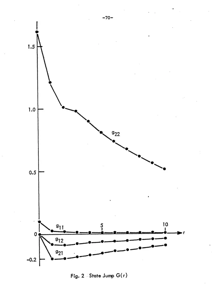
Figure 2. State Jump G(r) 70

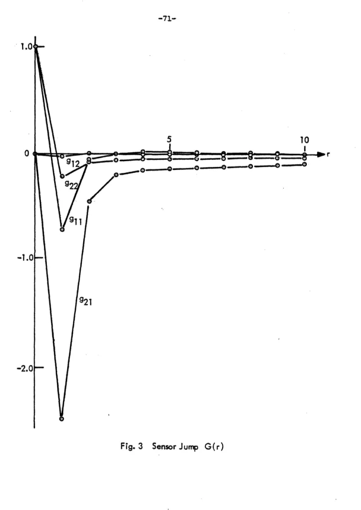
Figure 3.. Sensor Jump G(r) 71

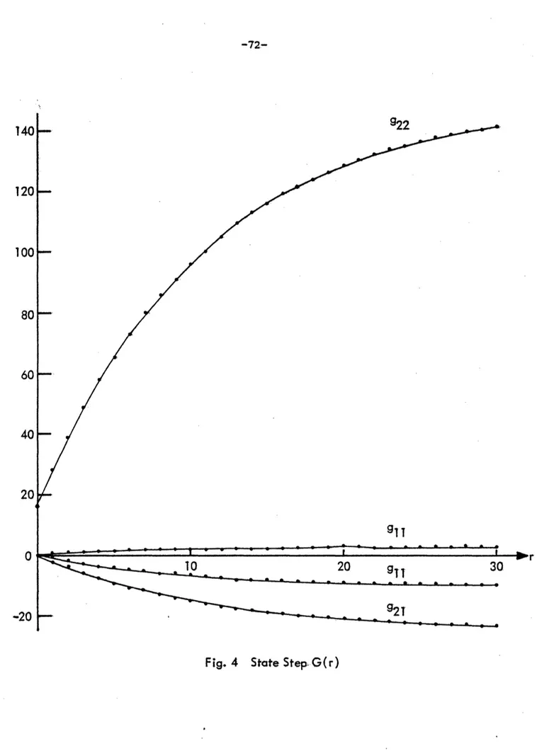
Figure 4. State Step G(r) 72

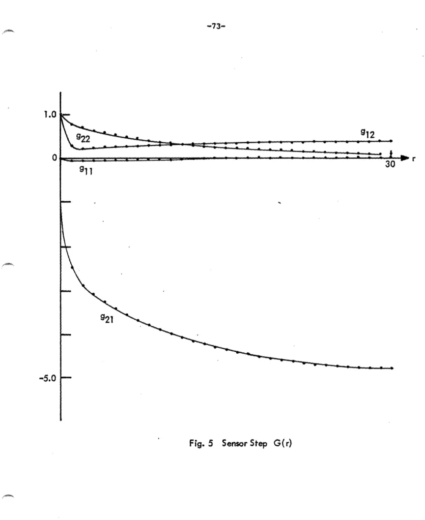
Figure 5. Sensor Step G(r) 73

Figure 6. State Jump C (r) 74

Figure 7. Sensor Jump C (r) 75

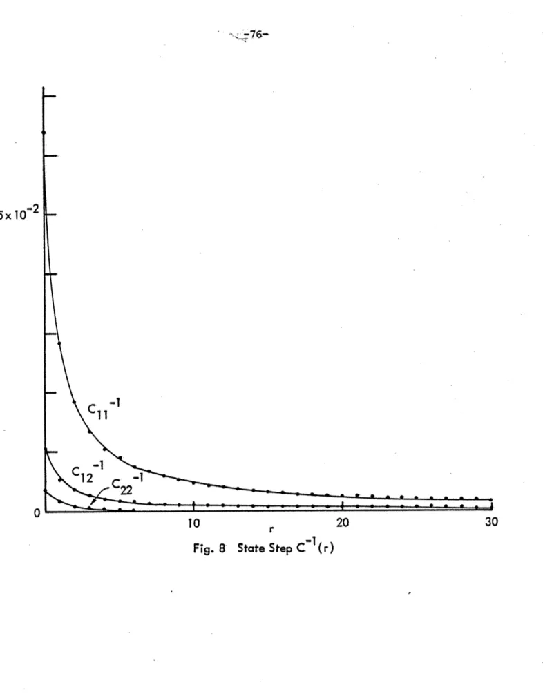
Figure 8. State Step C-(r) 76

Figure 9. Sensor Step C l(r) 77

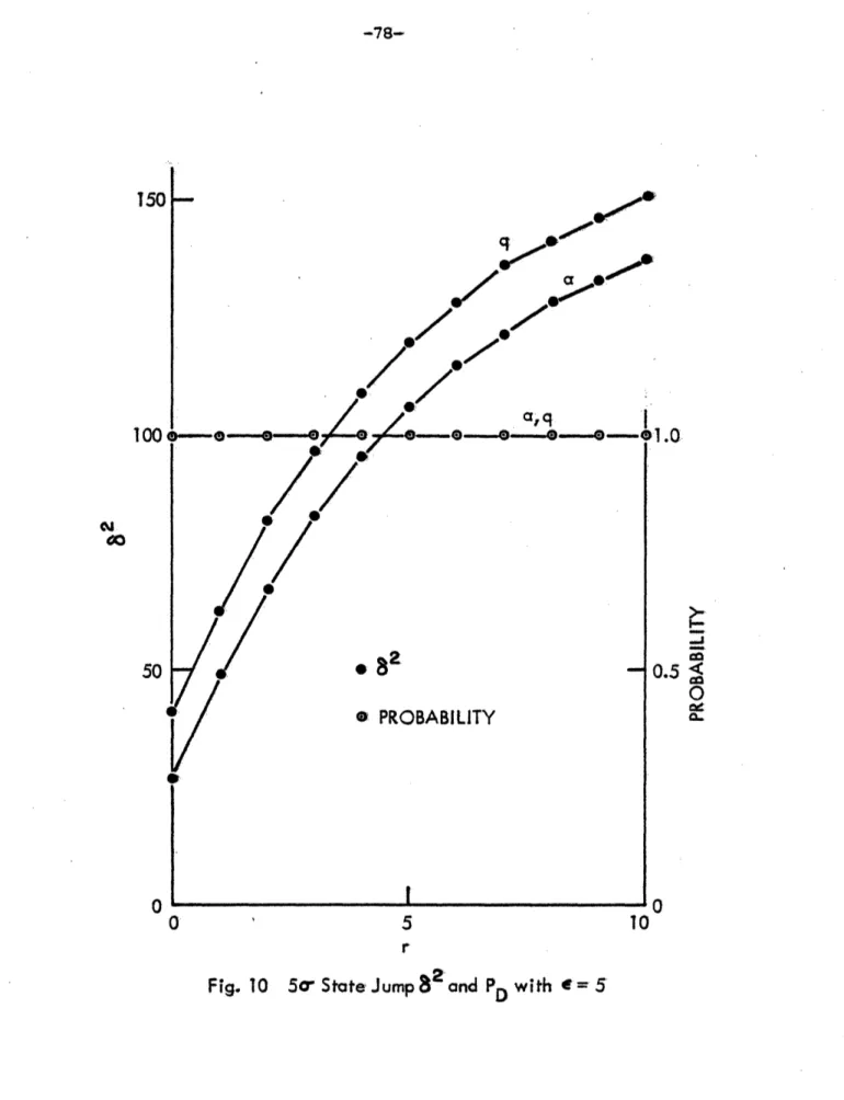
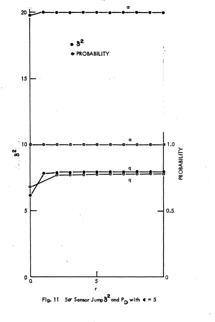
Figure 10. So State Jump 6 and PD with S = 5 78 Figure 11. 5a Sensor Jump 62 and PD with

s

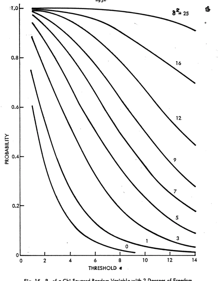
= 5 79 Figure 12. 1o State Step 65 and PD with s = 5 80 Figure 13. 1a Sensor Step 6 and PD with s = 5 81 Figure 14. Wrong Time Cross Detection Probability 82 Figure 15. Pk of a Chi Squared Random Variable with 2 Degrees

1.1 Motivation

Many aspects of recent developments of systems theory are con-cerned with the improvement of the performance of control systems. One such concern is the detection of abrupt changes in dynamical systems. Examples of abrupt changes are actuator or sensor failures in an air-craft and sudden changes in the rhythm of cardiac activities as measured on an electrocardiagram [6]. For simplicity, all such abrupt changes will be termed as "failures" even though a physical failure may not be

the cause of the abrupt change. The detection of failures may be viewed as consisting of three tasks: set off an alarm when a failure develops, then isolate the failure type, and estimate the extent of the

failure.

Most of the failure detection analysis has been performed in the context of a state space description of a linear dynamical system as

follows:

State Equation:

x(k+l) = D(k)x(k) + B(k)u(k) + w(k) (1-1) Sensor Equation:

z(k) = H(k)x(k) + J(k)u(k) + v(k) (1-2) where u is a known input, w and v are independent, zero mean, white

-7-gaussian random sequences with covariances:

E{x(j)w'(k)} = Q6jk ; E{v(j)v'(k)} = R6jk (1-3) where 6jk is the Kronecker delta.

Abrupt changes of the system may appear in (1-1) ("actuator failure") or in (1-2) ("sensor failures"). Actuator failures may take the form of a shift in the control gain matrix B, a bias on the right hand side (RHS) of (1-1) or a change in the process noise,

correspond-ing, for example, to the failure of the actuator or control surfaces on an aircraft, a leak in the thruster of a space vehicle and a sudden shift in wind conditions (in an aircraft control situation) respec-tively. In these cases, an accurate knowledge of the failure is clearly vital (assuming there is a re-organizational procedure to compensate for the failure), as an undetected failure could easily lead to the loss of the vehicle. Changes in sensor noise and the H and J matrices are examples of sensor failures. These are the causes of erroneous state estimates and produce very undesirable effects in a feedback control system that utilizes these sensor outputs in the feedback loop.

Recent studies have provided different approaches to the problem of detecting failures. The "failure sensitive" filter developed by Beard [1] and Jones [2], the voting system studied by Broen [3] and the multiple hypotheses filters employed by Gustafson, Willsky and Wang in the classification of rhythms and detecting rhythm shifts in electrocardiagram [6] are examples of some failure detection schemes. Very often, the tradeoffs among the various approaches are detector

complexity vs. detector sensitivity and detector sensitivity vs. detec-tor false alarm rate. Hence the applicability of the different schemes-depends on the particular situation and the performance criteria under consideration. With the decreasing cost of digital hardward and in-creasing availabiltiy of computers, many of these detection methods are becoming feasible for on-line implementation.

In [4], [5], Willsky and Jones have suggested the generalized likelihood ratio (GLR) approach to failure detection. As noted by

Willsky [9], the GLR approach can be applied to a wide range of actuator and sensor failures. The method also provides an estimate of the

failure size which is useful in system reorganization after the failure is determined to have occurred. The technique may be simplified in a number of ways making it more attractive from an implementation point of view. In addition, the tradeoff between complexity and performance may be studied analytically. In this thesis research, the GLR approach to

failure detection is studied to obtain insights into its limitations and to develop some guidelines in the design of GLR failure detection systems.

1.2 Description of the GLR Technique

The GLR failure detection system assumes a linear system des-cribed by (1-1), (1-2) and a Kalman Bucy filter (that assumes no failure) characterized by the following:

x(kfIk) -= ^(klk-1) + K(k)y(k) (1-5) y(k) = z(k) - H(k)I(kJk-1) - J(k)u(k) (1-6) where x(ilj) is the mean of x(i) given z(0), z(l), ..., z(j) and P(iij) is the associated error covariance. The quantity y is the zero mean, white gaussian innovations process (or the residual) with covariance V. K is the Kalman Bucy filter gain computed as follows:

P(k+ljk) = $(k)P(kIk)' (k) + Q (1-7)

V(k) = H(k)P(klk-l)H'(k) + R (1-8)

K(k) = P(klk-1)H' (k)V-1(k) (1-9)

P(klk) = P(klk-l) - K(k)H(k)P(klk-l) (1-10) The four basic failure types (modes) under consideration are modeled as:

Type 1: state jump

x(k+l) = $(k)x(k) + B(k)u(k) + w(k) + vSk+li (1-11) Type 2: state step

x(k+l) = $(k)x(k) + B(k)u(k) + w(k) + VSk+l;8 (1-12) Type 3: sensor jump

z(k) = H(k)x(k) + J(k)u(k) + v(k) + VSdke (1-13) Type 4: sensor step

z(k) = H(k)x(k) + J(k)u(k) + v(k) + Vk (1-14) where

1 if k = 8

kCi~~~~~ e

~~~~~~~(1-15)

Thus e has the meaning as the "failure time" and V is the failure vector of appropriate dimension. We note that the original GLR method devised by Willsky and Jones [4], [5] was developed for type 1 failures.

Due to the linearity of the system and filter, in the event of a failure, the residual can be expressed as:

y(k) = Y(k) + Gi (k;e)V (1-17)

1

where Y is the residual in the absence of any failure. G. is a matrix (i=1,2,3,4, denoting the failure type). The equations that one can use to compute the G. are given in Section 2.1. Then G. (k;O) is the effect of the type i failure V that occurred at time 0 on the residual at

time k. We can establish two hypotheses: H : no failure has occurred

Hi : a failure of type i (v and e unknown) has occurred.

Then the generalized likelihood ratio (GLR) is defined by p(y(l),..., y(k) IH.,

e

= 8(k), v = V(k))

L.(k) = .... (1-18)

1 p(y(l), .. , y(k)H ₀)

where p denotes probability density function; @(k) and V(k) are the maximum likelihood estimates (MLE) of V and

e

assuming H. to be true defined by:

i(k), V(k) = arg max p(y(l), ... y(k) H, i e = 8, v = v) (1-19)

0,v

-12-Given H. is true, the residual is

y(k) = y(k) + G (k;O)v (1-20)

1

for some unknown e and V. When H_o is true, the residual becomes

y(k) = y(k) (1-21)

Using the fact that the y's are gaussian independent variables and equations (1-20) and (1-21), the logarithm of (1-18) can be expressed as . i(k) = 2 Zn Li(k) k

=

_

y'

(j)v-y(j)

j=l k

E [Y(j)-Gi (k;O(k))V(k)vv (j) (j)y-G (k;e(k))V(k)] j=l

(1-22) To choose between H0 and Hi we use the decision rule:

H.

Zi(k) Z< (1-23)

H0

where £ is some predetermined threshold. Hence e(k) and V(k) also maximize Zi(k). Also, v(k) can be solved as-an explicit function of e(k):

v(k) C (k; e(k)) di(k; 6(k)) (1-24)

) is the matrix

k

Ci(k; 8) = Gi.'(j; ) V-(j)G(j; ^ (1-25)

and d (k; 8) is a linear combination of the residuals: k

di(k; 8) = Gi'(j; 8)

V-

(j)Y(j) (1-26)

j=l

Then 8(k) is the value of 8 < k that maximizes Z. (k;

8):--1

.i(k; 8) = d.'(k;

8)Ci

(k; 8) di(k; 8) (1-27)

Therefore, the GLR system (also known, for reasons that will become clear, as full GLR) will declare a type i failure V occurring at 8 if Zi(k; 8) > S and hi(k; 8) > i. (k; 8) for 1 < e < k. As time progresses, the number of possible values of 8 increases. Hence, the implementation of this scheme involves a growing bank of filters. (See Figure 1.)

When detectors for different failure types are implemented simultaneously, one is confronted with the additional problem of deciding among the failure types. A simple maximization of ,. (k; 8) over V, 8 and i may not provide satisfactory isolation of the failure type.- In the following, the subscript i is dropped for the sake of simplifying the notation.

A number of simplifications of the approach have been suggested by Willsky and Jones (5] such as the finite window assumption where 8

is restricted to a range, k-M < < k-N. The physical assumptions made here are: 1) no decision can be made with less than N observations (an observability constraint), 2) failures before time k-M should have been

*O z0_-LLa E E 0 O.2

O·

U-I ~~

~

0 0.-Z I_ C:.. . ' e . - I >

-i1,!~ ,,, i r iii i i i ii i i i iiiii iCi i iii ii

!O Q)

~

U

<N a:

U~O

0%o-

reasonable, and the resulting "sliding window" reduces the computational burden imposed by the growing bank of filters described earlier (where

calculation of Z(k; 8) for 8 = 1, ..., k is required). When the system under consideration is time invariant and the associated Kalman-Bucy filter (KBF) has reached a steady state, the G and C matrices become dependent on k-8 only. Thus, these matrices may be computed once and stored, greatly simplifying the required calculations. To reduce required calculations even further, one may wish to consider approxi-mating G and C (by polynomials, for example). Of course this will degrade the quality of the estimate of V.

Another simplification is the constrained GLR (CGLR) which in-volves the assumption that V = afj (where a is a scalar and fj is one of a finite set of directions). Thus, in computing v(k), we require it to be along one of these directions and estimate its magnitude (a). The CGLR detector takes the form:

A

^Ak b(k; 8(k), j(k))

a(k) = A^ (1-28)

a(k; 8(k), j(k))

where 8(k) and j (k) are the quantities that maximize

b 2 (k; 8,

j)

Z(k; 8, j) = (k; 8, j) (1-29)

where

b(k; 8, j) = f' d(k; 8) (1-31)

and d(k; 8) is defined by (1-26). The decision rule is:

H.

A >

Z(k; e(k), j(k) < s (1-32)

Ho

If V is further restricted to be some constant vo, one has the simplified GLR (SGLR). We note that SGLR does not require maximization over v and hence 2(k; e) becomes

k

£(k; 8) = E [2y(j) - G(j; e)v0] 'V 1(j)G(j; ;

0

0 (1-33)

j=l

Both CGLR and SGLR require less computation than full GLR. How-ever, they are directionalized, i.e., most sensitive to certain direc-tions only. This limits their ability to detect failure of other

directions. Consequently, they may be suitable only for a certain class of failure detection problems.

From the above discussion, it is clear that the GLR method offers a range of implementations from the point of view of computational

complexity. In order to develop a useful detector design methodology, one must study much more carefully the properties of the GLR method and the tradeoffs involved in the design. The purpose of this research is to study certain of these issues in order to provide some guidelines for the use of the GLR technique. Our aim is to develop an analytic framework in which one can systematically study the various tradeoffs

1.3 Overview of the Research

The two aspects of the performance of the GLR detector most closely examined in this research are the detector's sensitivity to failures and its ability to isolate the types of the failures. Effec-tively, the GLR detector concentrates failure information into the variable, 2(k; 8) as the decision rule considers only these quantities. Hence, a starting point in the analysis of the GLR detection scheme is

the study of this random variable.

In Chapter 2, we present the static analysis where we consider the Z's as static variables, i.e. the correlation among them is not considered. There, we derive expressions for probabilities such as the probability of correct detection and the probability of false alarm.: We also consider the questions of the detectability of failures by a GLR detector and the ability of the detector to, in some way, dis-tinguish among the different types of failure.

In Chapter 3, we study the correlation behavior of the Z's in an attempt to obtain more precise performance indices, such as the pro-bability of time to detection and to derive more information about the

failure from the temporal behavior of the likelihood ratios.

Finally, in Chapter 4, a summary of the study is presented along with a numerical example (failure detection for a simplified aircraft model) illustrating the performance of the GLR technique. We also

CHAPTER 2

Static Analysis

2.1 Summary of the GLR Equations

The implementation of GLR detectors requires the G matrices

described in Section 1.2. In this section, we present the equations

necessary for computing these matrices for the four basic failure types

(state jump,. state step, sensor jump and sensor step) as modelled by

equations (1-1l), (1-12), (1-13), and (1-14). The unfailed dynamical

system is represented by equations (1-1) and (1-2) which are repeated

here for easy reference.

x(k+l) = W(k)x(k) + B(k)u(k) + w(k) (2-1) z(k) = H(k)x(k) + J(k)u(k) + v(k) (2-2) The associated KBF: x(k+llk) = ~(k)x(klk) + B(k)u(k) (2-3) x(kJk) = x(kik-l) + K(k)y(k) (2-4) y(k) = Z(k) - H(k)x(klk-l) - J(k)u(k) (2-5)

where K is the filter gain computed from equations (1-7), (1-8), (1-9)

and (1-10).

Since the failures under consideration do not involve the known

control u, the control terms in the above equations may be omitted to

simplify the mathematics. However, the subsequent analysis is still

valid for cases where the control is present due to the following

reason. Since u is deterministic, its effects may be computed exactly;

-18-by linearity of the system and filter, the control effects may be added directly to the uncontrolled system and filter to obtain the controlled situation. Consequently, the analysis throughout this

report assumes the absence of controls without sacrificing the validity of the results for systems with deterministic controls.

2.1.1 The General Case

The linearity of the system and the KBF enables us to mathemati-cally decompose the residual y and the state estimate x(klk) into two parts:

y(k) = yl(k) + Y2(k) (2-6)

x(klk) = xl(klk) + x₂(k_lk) (2-7)

when the variables with subscript 1 denote the residual and state esti-mate when no failure has occurred and the subscript 2 denote the "bias" developed in the KBF due to failures. (Note that Y1 is the same as y defined in 1.2.) Similar decomposition is also applicable to x and z. In addition, we find that for the four failure types:

Y2(k) = G(k; 8)V (2-8)

x₂(klk) = F(k;

e)v

(2-9)

where G and F are matrices that are functions of the system and filter matrices, K, e and failure type.

After some manipulation of equations (2-3), (2-4) and (2-5), we obtain a recursive expression for x(klk):

kl) + k)Zk) 210)

-20-where

(k-1) = [I - K(k)H(k) ] B(k-1) (2-11)

To simplify some of the notations, we define

O(k, j) = 0(k-1)O(k-2) ... O(j) (2-12)

i(k, j) = ~(k-1) ¢(k-2) ... ~(j) (2-13)

Now, we are ready to consider the effects of the four types of failures.

State Step Failures

Consider a state step failure. Its effect on the system can be described by x2(k+1) = N(k+l, k) x2 (k) + ak+l,V , x2(0) = 0 (2-14) z2 (k) = H (k) x2 (k) (2-15) Thus z₂(k) = x₂(k) = 0 k <

e

(2-16) k x2 (k) = Z (k, i)v k >

e

(2-17) i=8 k 2(k) = Z H(k) b(k, i)v k > e (2-18) i=8

The effect on the filter:

x2(klk) = G(k, k-1) ₂ (k-llk-1) + K(k) Z₂(k), x2(010) =0 (2-19)

2(ktk) = 0 k < 8 (2-20) k x2 (kk) = 2 0(k,j)K(j)Z₂(j) k > j=e k j = E (k,j)K(j) H(j)4(j,i)V j=e i=e k k -= ~

X

(k, j)K(j)H(j) I(j,i)V (2-21) i=e j=i Hence x2 (klk) = F(k; 6)v (2-22) 0 k < e F(k; 8) = (2-23) 0(k,j)K(j)H(j)H (j, Z) k > e8 i-e j=i

From the definition of the residual (2-5), we have

Y2(k) = Z2 (k) - H(k)W(k, k-l)x2(k-l|k-l) (2-24) Y₂ (k) = G(k; 8)V (2-25) 0 k<e G(k; 0) = H(k) [

E

.(kj)-m(kk-l)Fk-i;6)] k > e (2-26)

Following similar calculations, we obtain the expressions of the F and G matrices for the other failure types [71.

-22-State Jump Failures

o0

Ik

< e

F (k; 8) = (2-27) k FE= e(k,j)K(j)H(j) (j, 0) k > (

j=e

O

k < 9 G(k; 0) = (2-28) H(k) £[(k,e) -( (k,.k-1)F(K-1; 0) k >

e

Sensor Step Failures

/

k <

e F (k; 0) = ) k (2-29) i (k,j)K(j) k > 9

j=e

(~~~~~0

k > e G(k; 0) I k = 8 (2-30) I-H(k) (k,k-l) F(k-1;

e)

k >

e

Sensor Jump Failures

[0 . k < e F(k; 0) = (2-31) O(k, 0)K(e) k >

e

k<0 G(k; 0) = I k = e (2-32) -H(k)~(k, k-I)F(k-1; ) > e

We note that the matrix G is essentially the only quantity that is needed in the implementation of the GLR detector. The matrix F is important in the implementation of a mechanism for compensation follow-ing detection. Examples of such a mechanism are discussed in [4] and are not pursued here.

Due to the fact that G(K; 8) = 0 for k < 8 and for all types of failures, the summation in the expression of C(k; 6) (1-25) need only be performed from j = 8 to k instead of j = 1 to k.

k

C(k; ) = G'(j;

8)V

G(j; 0) (2-33)

j=e

2.1.2 Steady-State, Time-Invariance Simplification

When the system (2-1) and (2-2), under consideration is time invariant and the associated KBF has reached a steady state, D(k) and O(k) become constant matrices D and 0 respectively. Then

G(k, j) = k-j (2-34)

D(k, j) = k-j (2-35)

Substituting (2-33) and (2-34) in the expressions of F and G, one finds, after some simple manipulation, that these matrices become dependent on the value k-e instead of k and 8 explicitly. Letting

r = k-0, we summarize the expressions under the steady-state time-invariance assumption in the following.

-24--State Step' Failures

0 k < e F.(r) = , (2-36) r r k >

e

i=0 j=i 0 k < e j=O

State Jump Failures

i0 k <9 F(r) = / r (2-38) k > 8 j=0 0 k < G(r) = (2-39) H ) Te - ~F(r-1)] k >

e

Sensor Step Failures

0 k< 0 F(r) = r (2-40)

)E OAK

k >e

j=0 0 k< 8 G(r) = k = (2-41) I - HF (r-1) k > e

Sensor Jump Failures 0 k < e F(r) = k

>(2-42)

r k k = 8 (2-43) -HOF(r-1) k > e

as defined in 1.2 becomes dependent on r (r = k-a):

r

C(r) =

E

G;(j)V- G(j) (2-44)

j=0

where V is the steady state covariance of the residual under no failure.

2.2 Static Probabilities

As some measures of performance of a detection system, the pro-babilities of correct detection (PD) , false alarm (PF), cross detection

(PCD) , wrong time (PWT) and time to detection (PTD) are defined as follows:

PD(k,

a,

8,

V)

A Prob ((k;8) > E1 , 8, v) (2-45)

PF(k,

a,

)

= Prob (Z(k;e) > cla, 8) (2-46) PTD(T,

a,

8,

v)

= Prob (Z(k;8) > s for some k < Tja, 8, v)

(2-47)

where ac is the actual type of the failure of size V and is. also the failure type the GLR detector hypothesizes, e is the true time of failure and e is the hypothesized time of failure. Also, we define:

PCD (k, a, S, , v) = Prob (Z(k;8) > sca,- a , 6, v) (2-49)

where a is the: failure mode the detector assumes, 8 is the actual failure mode, 8 and v are the time of failure and the failure vector respectively. We note that

PD a,8, , 0 (k, , ) (2-50)

PCD (k, at a, 8, v) = PD (k, a, 6, V) (2-51) PWT (k, a, 8, V, 8) = (I a, 6, v) (2-52) There are many aspects to the evaluation of a detection scheme and a single index is not sufficient to indicate the quality of the

scheme. The above defined probabilities are some convenient quantities defined to provide some insights into GLR detector performance. PD is a measure of detector sensitivity, since it is the probability of detecting a failure when a failure actually occurred. PF measures the negative quality of the detector, as it is the probability that a

failure is signaled when none has developed. Both PCD and PWT are more subtle measures of performance, since they pertain to the ability of the detector to distinguish failures of different types and different

failure times respectively. PTD is the probability of the time delay until detection and therefore is a measure of the speed of detection. This quantity is of obvious importance in evaluating detector performance.

Excepting PTD' these probabilities are defined at each point in time assuming no knowledge of the Z(k; 8) at other times. It is evident that the variable L(k; 8) is correlated with the values of 2(kl; El) for kl k and 8 8 . Thus a better set of performance measures may take this temporal correlation into consideration. PTD is an example of one such measure. The correlation behavior of the Z's will be investigated in Chapter 3.

In this chapter, we study the performance of the GLR detectors as measured by the above defined probabilities. The probability density of Z(k; 8) is shown in sections 2.2.1 and 2.2.2 to be chi squared (X2) and gaussian for full GLR and SGLR respectively. As the density is determined, the required probabilities may be computed relatively' easily.

2.2.1 Full GLR: X Probabilities

Consider a detector that hypothesizes a type i failure with

failure time = e while an actual failure v of type j occurred at 8_t. The actual residuals and GLR outputs then are given by

y(k) . y(k) + Gj(k; et)v (2-53)

k d(k; 8) =

L

G.'(s;8) -l(s)y(s) s=8 k =E Gi';)V l (s;)v(y (s) (s)+G (s; 9 t)v] (2-54) s=8 3 2(k; 8) = d'(k;8) Ci.i (k;818)d(k;8) (2-55)

-28-where

G. (k; 8) is the G matrix corresponding to & type fai.lure, y(k) is the unbiased white part of the residual, and

k

C.

1

.(k;

|eC) Gi' (s;v (siG.(5

e

8)

(2-56)

m"

G.r8

zv

Note that Cili(k;

e8e)

= Ci(k; 8) of a type i detector.

Since the sensor noise covariance, R, is symmetric and positive definite, V (m) is a positive definite symmetric matrix. Therefore, Cil i(k; 818) is positive semi-definite and symmetric. Then there exists an orthonormal matrix T such that

Aii (k; 616) = T Cjii(k;

818)T

(2-57)

where A.ili(k; 818) is a diagonal matrix and the diagonal elements are the eigenvalues X1 X2 '..' Xn of Cili(k; 818) (n is the dimension of

Cili(k; 818)). Assuming C jili(k;e 88) exists (we will consider this existence question later), define

Z(k;

8) = {d'(k; 8)T} {T-1Cii(k; 818 )T} {T-l d(k; )}

A -1

= v'(k; 8)A ili(k; 1) v'(k; 82) (2-58)

Then v(k; 8) is a gaussian random vector: k

v(k; 8) = T' Gi'(s:; 8)V (s!- [Cy() + G.j(s; t)v (2-59)

k

E{v(k; 8)} = T' Gi'(s; 8)V )G(sj(; ₈t) - T'CiCj(k;

818et)v

E{v(k; 8)v'(k; 8)}

= T'Cili(k; 8el)T + T'VCilj(k;

8let)C'iji(k;e81

t)v'T

= Aili(k; 61e) + [E{v(k;8)} [E{v(k;e)}]' (2-61)

Hence Aili.(k; e18) is the covariance of v(k; 8). Since

Ai i(k; 818) is diagonal, elements of v(k; 8) are independent of one another. Also, Z(k; 8) can be expressed as the summation:

n 2

v (k; 8)

2(k; e) = E s (2-62)

s=1 s

where v (k; 8) is the sth component of v(k; 8). Then each term in the above summation is the square of a gaussian random variable with unit

V (k; 8)

variance and mean of s (v (k;e) is the mean of v (k; 8)). Xs ss2

Therefore, Z(k; 8) is a noncentral X random variable with n degrees of freedom [10]. The noncentrality parameter (62) can be computed as

follows.

n -2

v_s (k; 8) 62 A s

s=l S

= [E{v(k; 8)}]' Ail.(k; 01e) [E{v(k; 8)}]

= VC j.(k;-

let)

Cij.i(k; 818) Cilj(k; e81t)V (2-63)

The expected value of k(k; 8) is then simply n + 62.

Note that no assumption is made on i, j, 8 and e_{t .} The deriva-tion includes the condideriva-tions defining PD' PF' PCD' and PWT as special

-30-instance, i may be different from j while 8 is: different from Et (but

the G"s are computed according to the same system and filter). This corresponds to a case of wrong time cross detection. and it could be

of interest. The associated probability (of wrong time cross detection)" may be greater than the probability of Correct time cross detection

implying that a mismatched failure is- more likely to be regarded as a matched failure but at a failure- time different from the true one. In any event, Z(k; 8) is a noncentral X random variable with n degrees of freedom and a noncentrality parameter 62 dependent on the conditions hypothesized..

Specializing to the four cases of current interest, we have,

Correct Detection 8 = 8, i = j 62 =V 'C. i(k; e08)v (2-64) False alarm i = j, V = 0 2 6 =0 (2-65)

Z(k; 8) becomes a central X random variable Cross Detection

i j,

e

= 8t

62 = 'C

lj(k; el1)C

(k; i)Cj (k;8le

)v

(2-66)

Wrong time

i= j 0 e fet

~----t---Note that the different relationships among 0, 8t, k have different

physical interpretations, for instance,

k < it <

a

k < e < 8t j not meaningful t< k < e 8 < k < e_t false alarm 8 t t > wrong time (2-67)

e

<

<

k

X

then under the wrong time assumption and (2-66),

2 = V'C (k; 010t)Ci

i(k;

el

ec

i (k; 1eet)v (2-68)

The probabilities, PD', PF PCD and PWT can be computed by simply integrating the chi squared densities with the appropriate degrees of freedom and noncentrality parameters from Z = s to Z = +c. There are

computer subroutines for computing central X2 probability [13]. An algorithm for computing noncentral X probabilities has been developed and is described in the appendix.

2.2.2 SGLR: Gaussian Probabilities

Consider a simplified GLR detector set to detect a failure V0 of type i with failing time e while a true failure V of type j

actually occured at t, The actual residuals and log likelihood ratios are given by

-32-y(k) =y (k) + Gj(k;

et)v

(2-69)

k

Z(k;) - E [2Y(s)-Gi(s;8) O'V - (s)Gi(s;8) ₀ s-e k =- 2y'(s) V (s) Gi (s;))O s=6 k + 2 L V'Gjt(s;et)V (s)Gi(s;e)v0 s=8 k -. VO Gi ' (s;6)V- (s)Gi(s;)V 0 s=8 k -C 2 V' G.'(s;O)v (s)y(s) s=8

+ 2 V0' Cilj(k; -let) - Vo' Cili(k; I ) ₀ (2-70)

Since y(s) are zero mean, independent gaussian random vectors, 2(k;e) is a gaussian random variable with mean (m) and variance (a 2):

m = E{t(k;8)} = 2V'Cilj(k; 8It) - vO'Cii(k; I)v 0 (2-71)

2 2

a = E{([(k;O) - m]

}

=4 O[ · EF~ Gi'(m;e)V' (m)Gi(m;e)] V0

= 4 V01 Cili(k;G)V0 (2-72)

Note that the variance is the same for all cases whereas the mean varies.. For the four cases of interest:

Correct Detection

i

=

j,

8

S=etr

,

V

0

O

m = VO' Cili(k; 18 ) V0 (2-73) False Alarm i = j, V = O m - -V₀' Ci_{l i}(k; 818) V0 (2-74) Cross Detection i ~ j, V

j

VO, 0 = et

m= 2 V₀ ' Cilj(k;

e6e)V

0VO'

-

C1i(k;

ele)

0 (2-75)

Wrong Time

i = j, V = VOl

8 < et < k or et < < k

m=

2

V₀

' Cili(k;

ejet)V

-

V

C.iili(k;

IOe)v

₀

(2-76)

Then the desired probabilities can be obtained by integrating the appropriate gaussian densities. This involves the evaluation of error functions.

2.2.3 Discussion

For chi squared densities, the probabilities PD, PD ' P are increasing functions of the noncentrality parameter 62 for a fixed threshold e (see Figure 15 ). For SGLR, a similar relation between the probabilities and the mean of Z holds. The variance of the

likeli-

-34-hood ratio of a SGLR. set to detect a particular failure is a constant for all. different time failures. Only the mean m varies with the time failures. Hence, both 62 and m are Calternative measures of GLR

per-formance..

When considering PD, 62 takes the form v'C(k;e)v, where V is the true failure. Then for any threshold, the probability (P D) of detecting

2

this failure V is directly determined by the effect of V on- 6 . The failure becomes more "detectable" as V results in a larger 62 and con-sequently a higher PD. A zero 62 will make PD equal PF signifying that the detector is unable to tell between. the- failure and the noise in the system. Hence, a failure v that occurred at

e

is viewed as "undetec-table" at time k if V'C(k;6)v (the 62 for computing PD) is zero.

Simplified GLR behaves in a similar manner.. In considering PD for SGLR, a is 2 I, and thus _ = v (which represents effective

D ft GR . n h m 2

SGLR signal to noise ratio). Hence, an increase in m will give a

larger PD for any threshold. The only difference is as follows. Here, the mean value (m) of the likelihood ratio takes the same form as 62 for full GLR. A failure V that causes a zero m will make a zero and consequently Z(k;e) zero deterministically and independent of the residuals. In this case, failure detection is clearly meaningless.

As the C matrix is closely related to the detectability of failures, it is studied in section 2.3 to explore its significance and behavior as functions of k and 6. In section 2.4, the C matrix is examined to determine undetectable failure directions.

After consideration of PCD and PWT similar to that of PD in the above, we note that the d2 associated with these probabilities and

con-sequently the Cilj matrix are crucial factors of the detector's ability to "distinguish" between different failures and failure times. This issue is further explored in section 2.5.

2.3 The Information C Matrix

The C matrix is called the failure information matrix for reasons that will become apparent. In addition to its- relation to the proba-bility of correct detection, the C matrix has one other important

-i

property. In section 2.3.1, we will show that C (k; e) is the error covariance of the MLE of the true failure assuming that the full GLR detector has determined the true failure type and failure time.

The general time varying situation is too complex for initial analysis. To obtain some basic understanding of the behavior of C(k;8) as a function of k and

e,

we have turned to the time invariant, steady state situation. In 2.3.2 we will discuss the asymtotic behavior of

C(k-e).

2.3.1 C (k;e): the. Error Covariance of v

Consider the situation where a full GLR detector has determined the type of a true failure V and the true failure time

e.

Then the MLE of V is V as described by equation (1-24).

-36-For easy reference, we repeat the definition of C and d here. k C(k; e) .. G'(j; 0) V l(j)G(j; 0) (2-78) j=e k d(k; ) = G'(j; )v-(j)y(j) (2-79) j=0 where

y(j) = y(j) + G(j; e)v (2-80)

The actual residual y contain a zero mean white independent component y with covariance V and a bias G(j; 0)v due to the actual failure. We

also define

k

d(k; 0) = G'(j; )V- (j)Y(j) (2-81)

j=0

The d is also zero mean, white independent with covariance:

E{d(k; 0)d'(k; 0)} = C(k; 8) (2-82)

Furthermore, we have

d(k; 0) - d(k; 8) + C(k; 0)v (2-83)

We can compute the error covariance of the MLE V as follows:

E{(v - V)(V - v)'} vv' - E{Vv'} - ECvv'} + E{vv'} (2-84) Second term on the RHS of (2-82):

E{VV'} = E{C l(k;0)d(k;6)v'}

= E{C l(k;e) d(k;0)v' + C (k;0)C(k;0)vv'}

Third term:

E{VV'} =- E{VV'} = VV' (2-86)

Fourth term:

E{VV'} = Et{C (k;8)d(kdI(k;8)C (k;)d(k,)

= C-l(k;8)E{[d(k;e) + C(k;e)] [d(k;8) + C(k;)v]'}C -l(k;8)

=C 8) E(k;) E{ d(k;)'(k;) + d(k;8)v'C(k;e)

-1 -1

= C (k;6) [C(k;8) + C(k;8)vv' C(k;8)] C (k;8)

= C 1 (k;8) +vv' (2-87)

Summing up the terms,

E{(V - v) (v - v) '} = C (k; 0) (2-88)

Under the assumption that the full GLR detector has decided on the true failure type and failure time (0), we have shown that C l(k;0)

is the error covariance of the MLE of the true failure. From the

theory of linear algebra (16] we know that both C and C-1 have the same eigenvectors and that these eigenvectors are orthogonal to one another since the matrices C and C-1 are symmetric. Suppose a failure v lies in the direction of an eigenvector xl of C corresponding to a large eigenvalue X₁ ( >»> 1). Then 62 ( = v'Cv) and PD for this failure is

1 D

large. The error covariance of the MLE of V is (= xC xl) which-1 is small. The failure direction xl is a detectable direction as it can be detected easily as well as estimated accurately. If V lies in the direction of an eigenvector x2 with small eigenvalues A2 (X2 << 1),

-38-the associated 62 is small andconsequently PD is close to PF, In

-1

addition, the error covariance of the MLE of V, X₂ , is large. Hence, the failure direction x2 is "less" detectable. Indeed, the matrix C

describes the directional sensitivity of GLR.

We will describe a failure direction as undetectable if it results in a zero 62. Thus a direction is detectable if it produces a nonzero 62~ In order to gain insight into the detection problem, it is appro-priate to study the subspace of undetectable directions (which is similar to the concept of unobservable subspace in linear systems). By- under-standing it one can provide an analytical foundation for questions such as the distinguishability of various failure modes. Note that the set of detectable directions is not a subspace and two directions are-totally indistinguishable if they differ by an undetectable direction. With this idea as a foundation, one may be in a position to define a concept of distance between failure directions -- i.e., a measure of the degree of distinguishabiliy (see section 2.5).

For full GLR, we have assumed the existence of C . (Otherwise, a pseudo inverse may be used [5].) When C is noninvertible, it must have some zero eigenvalues. If we allow some eigenvalues of an invertible C to approach zero, the noninvertible situation is reached. By a limit argument, the above discussion may be extended to a noninvertible C matrix and hence leads to the notion of undetectable direction mentioned earlier. The relationship between invertibility of C and detectable failure directions is further examined in 2.4.

2.3.2 Asymptotic Behavior of C(r)

In a time invariant system, C(k; 8) becomes dependent on the difference between the true failure time and observation time (k-8). For convenience, we let r = k-8. Furthermore, we assume the associated Kalman filter has reached a steady state. The four different types of detectors are considered separately.

State Jump Detector r

F(r) = E r - j KiH j (2-89)

j=0

where

e

= (I - KH]J; K is the steady state Kalman gain, ~ is the system matrix and H is the observation matrix.

Both the system and the filter are assumed to be stable. Then the magnitude of the eigenvalues of ~ and 0 is strictly less than 1, i.e.

|Ii(D)I < 1 i = 1, 2, ... n (2-90)

Xi(

l

1 i 1, 2, . n (2-91)

where Xi(Q) and Xi(0) denote the ith eigenvalues of d and 8 respectively and n is the dimension of ~ and O. Consider the norm |

j|

of an nxm

matrix A, 1

AJi

=!max (x'A.'Ax)2 (2-92)

where x is an m-vector.

For a square matrix A with all eigenvalues of magnitudes less than 1, it can be shown that 11 AlI 1.

-40-For a jump in the state,

r F(r) = E: .rjm (2-93) j=0 r r j=0 j=0 =

IIKHII

(r+l)pr

11··11

il~p'

(2-94)(2-94)

where p

= max'

{|II|l

, 11011)}

Since p < 1, there exist an a >

O0

such that p = e . Then

IIF(r)

I

<

II

KH|I

(r+l)e

(2-95)

The RHS goes to zero as r + -. Therefore

lim F(r) = 0 (2-96) r -> oo Similarly, for G(r), |IG(r) | = | (Hr - ~F(r-1)]II

_1 1

1H

1

_{I 1'1}

+

₁

_IlF-11|

<

IIHI

t[pr +

IIIII1

rPr] (2-97)

Hence G(r) also approaches zero as r + o. Now consider C(r). Define

AC(r,s) A C(r) - C(s) , r < s

-= G'(j)V G(j) (2-98)

SI

Ilac(r,s)l|

<

EI1i

' lv- 11

!

[pj +

1H!

!

jpjI

j=r+l

<

I Iv-

11

IH11

2 _[(c-r)pr

₊

_{|IKHI! (s-r) rprlr}

(2-99)

As r + a, the terms in the bracket approach 0. Hence

lim |JjC(r, s)jj = O r < s (2-100)

This showsthat {C(1), C(2), ... C(r) ...} is a Cauchy sequence and hence

converges to a finite constant matrix. This has the implication that

62 in the state jump case will approach a finite limit; as this limit is reached, we are getting no more information about the jump from y.

Thus, waiting further will not improve PD nor the error in the failure

estimate. Therefore, the rate of convergence of C(r) to its limit may

be used in determining the length of the detector window (i.e., the value of M for the window: k-M <

e

< k-N).

Step in the state

r r r j

F(r)

E

Or-j

KH¢J-i =

:

Gr-1

E

KHi

i=O j=i j=0 i=O

r

E 8r- j KH[I-_[I-]-j+] l

j=0

r r

= L

er-j

KH[I-_]- -_ ₀r-j KHBj+l [I_ ] -i

-42-= r [ [I -]KHI -][ - 1

i

er-JKHJ

Ir--

l

(2-101)

j=-As- r -+ , the first term becomes: [I-0e] KH[I-I- '1 and the second goes to O following the reasoning for the state jump case.. [I-G 1 l and

[I-4]- 1 exist because I|i(@)

1<

1, IXi() I < 1 for i = 1, 2, ... n.

r

G(r) = H

[

L r

j _-

F(r-l)]

j=0

= H[I-[r+l] [I] - 1 - HDF(r-l) (2-102)

-1

As r - a, the first term becomes H[I-]1 and the second,

HwU[I-0] iKH I-J 1- . Hence G(r) reaches a constant, H{I-fI-O]- 1 } [I-¢]- 1 -as r - m. G' (j)V- G(j) is positive semi-definite and attains a steady state value G' ()V iG(-). Thus at least some eigenvalues of C(r) grow as r increases indicating that some failure vectors will cause a growing 62. Therefore, an actual failure lying in the direction of an eigenvector of G'!()V-G(-) with a nonzero eigenvalue will cause PD

to approach 1 as the waiting time (r) increases.

Jump in Sensor

lim PCr) = lim R = (2-103)

r X r+ r li X2

lim G(rl = lim -HPF iO1J = 0 (2-104)

Hence sensor jump C Cr1 Behaves much like that of state jump failures: C(r) approaches constant as r approaches a.

Step in Sensor r lir F(r) = lim E JK r - r >X J=0 (2-105) = [I-1] K

Iim G(rl = lim [I-HOF(r-1)] r += r +"

(2-106) = r-H ([F1]' K

Therefore, the sensor step C(r) behaves in a manner similar to that of the state step C(r) as r approaches A.

2.4 Undetectable Failure Directions

One moment's reflection upon the physical meaning of an unde-tectable failure leads us to believe that a failure is not deunde-tectable if it cannot be observed by the system's sensors. Therefore, state failures that lie in the unobservable subspace are not detectable and all sensor failures are detectable as they have direct effects on the sensor outputs. From the discussion in 2.3.1, all failure directions are detectable if C is positive definite (i.e., invertible). Now we will determine the

condition for C to be invertible under the time invariant steady state assumption.

The positive semi-definite synmetric matrix C(r) may be re-written as

-44-GCrl = IG"

CO

:

G(

G, C

:

..-

G

"

(r:

-I

-

[

CO

0 V IG (1)

a

.

"

r

)

'V-' LGi

i]

G; (r) VG (r _(2-107)

Since V is positive definite, V is also positive definite. It is clear that C(r) is positive definite if and only if the null space of G(r) is {O}. We will examine G(r) for the four different failure types separately.

State Jumps,."

After some manipulation of the expression of G(r) (2-39), we can w*ite G(rl as a product of two matrices:

G(rl

=-H

I 0o

=t

rK

HE)2K Ar HBr)

AlCr) is a lower triangular matrix with identity blocks on the diagonal and is thus of full rank.. On the other hand, the null space of B(r) is the null space of G(rY. We note that BV(r) B(r) is the observability

gaussian.. Therefore, C(r) is positive definite if the system is observable in r steps. Since the unobservable subspace in r steps is the null space of B (r) and G(r), the observable subspace coincides with the "undetectable subspace". One other property of system observability maybe applied here, i.e., if an n dimensional constant system is not completely observable in n-l steps, it will never be completely observable. Then if C(r) of an n dimensional system is not invertible for r = n-l, it will not be invertible for r > n-l. Hence, after waiting n-l steps (r = n-l), the undetectable subspace becomes constant. However, C(r) may be noninvertible

for r < r0 but invertible for r > rO and r < n-l. These last two

pro-perties of state jump detection may be used to determine the value of N in the window k-M < 0 < k-N.

That is, if a jump V is in the nullspace of C(r-l) but C(r)V # 0, we will certainly take N > r when looking for a jump of this type. In

SGLR and CGLR (where we prespecify failure direction), we will set different window constraints for different jump directions, depending upon their

observability. In full GLR, the failure direction (as well as magnitude) is determined on-line. One obvious design concept for full GLR is to choose N large enough so that C(N) is invertible (assuming the system is

-46-we choose N such that det C(N) = Q, we must take care in utilizing the full GLR equations given earlier, That is, we must replace C ' by a pseudo-inverse and should take- care in making sure that V lies in the orthogonal complement of the nullspace of C (as it will if we use the standard Penrose inverse).

State Steps

G(r) =

0I OK I p W0

I-HQDK HW

r-l r-2

I-H Z &K I-H5 G C2K I.. H

j=0 j=O

A2(r) B(r) (2-109)

Ar(r) is of full rank. B(r) is identical with that of the state jump cases. Therefore, similar comments applies here also.

Sensor Jumps and Steps

Upon examining the expressions of G(r) (2-40) and (2-41) of these two failure types, we find that G(O') = I for both types. Consequently, the null space of G(r) is {0} implying that C(r) is always invertible for sensor failures.

-The above discussion on state jump, senior jump and sensor step failures maybe extended easily to the general time varying cases. It is clear that in the state jump case, observability has to be considered for a time varying system and the value of r for which C(k; k-r) is in-vertible will generally vary with time k.

For state steps in an n dimensional time varying systems, the in-vertibility of C(k; 8) is related to the observability of an augmented system. An n dimensional system with state step failures (2-110Q (2-111) can be represented by a 2n dimensional system with state jump failures

(2-112) (2-113).

An n dimensional system with state step failure

x(k+l) = ¢(k) x(k) + vk+le (2-110)

z(k) = H(k) x(k) (2-111)

An augmented system with state jump failure

x(k+lf _1 (k) IX x (k+), o

[lktlj ,

LI

[x

L

l)J + [0] k+1 G-1 (2-112)

z(k) = [H(k) 0] x(kj (2-113)

Recall that in the state jump case, a failure direction is undetectable if it lies in the null space of the corresponding C matrix, Then, jump

-48-if they do not lie in the null space of the state jump C matrix of the augmented system, Therefore, we deduce that the state step C matrix of the original system is invertible if the null space of the state jump C matrix and hence the unobservable subspace of the augmented system does not contain directions of the form t[0, V] .

Furthermore, we have made the following observation. Suppose all state jumps in the original system are detectable. Then if some state jumps in the augmented system are not detectable, we know either or both of the following are true:

1. At least some state steps in the original system are undetectable.

2. Certain state steps cannot be distinguished from jumps in the original system, e.g., consider the 2 dimensional system

x(k+l) = 1l 1 x(k) (2-114)

° 1

x(k) = [1 0] x(k) (2-115)

This system is observable hence all state jumps are detectable. But a jump in the second state. is indistinguishable from a step in the first. A check of the observability grammian of the augmented system shows that the augmented system is not completely observable i.e., some state jumps here are undetectable.

2.5 Distinguishability of Failures

Recall that when the likelihood ratio crosses the threshold, a failure is declared: in full GLR, a failure (size and direction unknown) of the type hypothesized is declared while in SGLR, a failure of the hypothesized type and direction (size unknown) is declared. However, there are many possible causes of the likelihood ratio's exceeding the threshold e.g., a noise spike, an actual failure of the hypothesized type or another type of failure. Therefore, failures other than the ones hypothesized by the detector can be mistaken as the hypothesized

failures. The sensitivity of a particular detector to other types of failures makes it difficult to distinguish between various failure modes. In this section, we will make a first attempt to consider this problem analytically in order to provide basis for detector design and reliability analysis.

Consider a SGLR detector that is set to detect a failure in the direction fl of type i. Then the probability of detecting fl when it occurs is PD' In the event that another failure in direction f2 of type j occurs ,the probability that the SGLR declares a failure in the direction fl of type i is PCD Clearly the quantity PCD provides a measure of how distinguishable various failure modes and directions are.

If PCD < Pp' the modes are distinguishable. If PCD >-- the modes are correlated and the size of PCD is a measure of the degree of the indis-tinguishability between the failure modes.

-50-Since full GLR is sensitive to failures in all directions of the

specified type, we should only consider the distinguishability of

dif-ferent failure types. Suppose we have a type i full GLR and a type ....

failure of size f occurs. Since full GLR will choose the most likely

failure direction Let· us find the direction v of type i failure for

which SGLR has the highest PCD under the failure f. Then this highest

PCD is a measure of how distinguishable the type of failure of size f

is to full GLR of type i. To obtain this quantity, we need to maximize

PCD over all directions v. Thus it is clear that full GLR will have more

complicated distinguishability problems than SGLR. The analytical study

of these problems is beyond the scope of this thesis. But we will.

con-sider SGLR as it should provide insights into the problems in full GLR.

Although the foregoing discussion concerns the cross detection

situation, the same reasoning is applicable to wrong time detection

where PWT is the measure of distinguishability between true and

hypothesized failure times. A more general situation is the wrong time

cross detection. This is also an important case. The physical

in-terpretation of the situation is that a particular failure mode may

not look much like another one occurring at the same time, but it

may be highly correlated with the other mode started at a different

time (e.g. ,sin(w.t+8e)is uncorrelated with cos wi.t for 0=0 but they are

highly correlated for e8--/2). In the following, this general case is

considered and the wrong time and cross detection cases may be regarded

as specialized results of this general one.

2

and variance _{ml/1 =} (a1) _{VL Ci/i(kEl/0l)vl} of · L(k;e ) of Dl when Vl occurs at 81 are given by_{(2 116)}

a, 4 ml/l (2-117)

In the event that another failure V2 of type j occurring at

82' the variance of t(k;81) of DI is still a1 while the mean is

ml12-m1/2 = 21' Ci/j (k;81/82)V2 _m. (2-118)

We define

m1,₂ =I Ci/jik;el/e2) 2 (2-119)

Then it follows that

m₁ = m₂,1 (2-120)

mljl i n, ₁ (2-121)

For a fixed threshold, PCD is an increasing function of ml/2, or equivalently, m1,₂ (as m/11 is fixed for D1). Therefore, ml,2 is

a key (wrong time) cross detection parameter and a measure of dis-tinguishability.

-52-k

Ci/j (k;

8

1/ 2) = E Gi (s;) V(s) Gj(s; 2 (2-122)

Since for k < 8 and i = 1,2,3,4,

G. (k;e) = 0 (2-i23)

equation (2-122) may be expressed as k

Ci/j (k;0/2)

=

G.(s;i 1) V-l(s) G (s;0 (2-124)

s=8 where

e = max {l, 82} (2-125)

Then we can express im, ₂ as

r 1

,

2

= V'[G

'(;0

1

).Gi

(0+;

).

' (k;

V (e)

V-1

(e+1)

x

V_-1(k) -G (e;82) G. (e+1;02) V2 G (k;82) 'Gt (k;8;8

1)V(k;e)

Gj(k;e;82) V₂ (2-126) 1 i~~~~~~~~~~~~~~~~~~~~~~~~~~~~~~~~~~~~~···--- ···-r·-··---·-·-·- --

---Since V(k;e) is a positive definite matrix, ml,2 is in fact an inner product:

ml,₂ <Gi(k;6;1))VG 1, G(k;;8 2)v > V(k;e) (2-127)

To simplify notations, the explicit arguments of Gi and Gj are suppressed

in the following. Hence

mln₂ < GiV ₁ Gjv₂ > V(k;e) (2-128)

m1,2 = i '

j

Now suppose that a second SGLR (D2) is set up to detect the failure V2. When v2 occurs at 82 the mean (m2/2) and variance (a2) of t(k;82) of D2 are:

i2/₂ V '2'Cj/j(k;82/82) v2 (2-129)

2

2_~2 = 4 ₌ m2/2 _{4 m2/2} (2-130)

If in reality V₁ occurs at 6, instead of v₂ at

e

, ₂ the variance of t(k;82) of D2 is still a2 but the mean is m2/1:

m2/1 = 2v2 Cj/i(k;821 1)V1 -m 2 / 2 (2-131)

If we assume that we design the magnitude of the assumed failures V₁ and V2 so that

-54-we than have equivalently set the P 's of both SGLR (D1 and D2) to be equal. Physically, this means that at time k, D1 is as sensitive to V₁ that occurred at 81 as .D2 is sensitive to V2 that occurred at 82.

From the Schwartz inequality, we have

(2-133)

2

Gv

<i i 2Z (k;cce)<G V 1 Gi 1> V(k;) < Gjv2 ' j2 > V(k;0)

A closer examination of ml/1 is appropriate here, By equations (2-121) and (2-127), we have

ml/1 = Gil' Gil> V(k;0) 2-34

If 81 = e, then

ml/i = <Gi1' Gini> V(k;8) (2135)

Suppose 81 < 8, then

(2.136)

0-1 k

ml/l = vl 1 Gi (s;01 )V(s) G. (s;e1) + Gi (S;0 1)V(s) Gi(s;0)l]V

s=e s=8

The second term in the bracket is actually <G.vl, GiV1>(k. Since the first ferm in the bracket is a positive semi-definite

matrix,-nml/ > <Giv₁

,

Givl> V(k;6) (2-137)

Both 2135 and 2137 su arized in (2-137(k;)

Then we have

ml,2 <ml/l (2-138)

(2-139)

1,2 m2/2 (2-139)

Now we have arrived at the following result. For a fixed thres-hold e that is common to both Dl and D2, the failures V1 at 81 and

V2 at e2 resulting in the same mean value for the t of their matched

detectors (dl and D2 respectively) will give the same PD' Furthermore, the wrong-time, cross-detection probabilities of both detectors (with

respect to the above failures) are not greater than PD. From another point of view, this result -- i.e., the cross correlation (2-127)

provides a measure of the degree of indistinguishability between failures (and failure times) under the assumption (2-134). This result may be extended to include cases of more than two detectors and provides a

first step for the development of method for designing "mutually dis-tinguishable" detectors.

It is desirable for the mutually distinguishable detectors to have the same PD and PF for all times. This means that we can detect

smaller failures in the "more sensitive" directions as well as we can detect larger failures of "less sensitive" types and directions. We note that the sensitivity of SGLR to different type and size failures

varies with time (depending upon the shape of the GV 's). In order to

-56-to scale the V's of the SGLR detec-56-tors in a time-varying manner. This can be done by normalizing the G's appropriately. This problem is an interesting one for future research.. In addition, once mutually distinguishable directions are dtermined, one will probably find it more useful to use constrained GLR tan full GLR. This question is also of interest for the future.

In the previous chapter, we have derived some properties of the GLR failure detection system by studying the statistical properties of Z(k; 6). The likelihood ratio Z(k; 8) was treated as a static variable, i.e. it was regarded as a function of the fixed time parameters k and 8. The Z's at different k's and 6's are clearly correlated. Hence the study of the correlation is important in the understanding of the behavior of the i's with respect to k and 6. This will clearly be

important in the development of a reliable detection rule. In full GLR, Z(k; 8) is a X2 random variable and the correlation study of such vari-ables is difficult. However, SGLR provides a very manageable situation as the Z's are gaussian random variables. Thus we will focus mainly on the correlation of the Z's in SGLR. In section 3.1, we will derive

the covariance function. Some additional probabilities such as PTD and their computations are discussed in 3.2. As the behavior of the Z's as functions of k and e are known, possible modified decision rules for GLR failure detection systems are discussed in section 3.3.

3.1 The Covariance of Z(k; 8)

Consider two likelihood ratios of a SGLR detector at different k's and 6's under a certain failure condition. By equation (2-69), these Z's have the following expressions:

-57- -58-kI 2l(k; 8₁) 2 G! (s; 8V1 '(s)y(s) + ml(kl,el,t,V,_{j )} k2 (3-1) Z2(k2 62) 2 V

E

G!(t;06)V (ty(et) + m2(kt 2 e 1Q j) t=2 (3-2)' where y is the zero mean, independent, white gaussian sequence, e_t is the true failure time of the type j failure v, and the m's are the expected values of the Z's as given by (2-71).

The cross covariance (R₁₂) of Z1 and k2 can be simply computed as:

R12 =E{(Zi1 - ml)9(2 - m2)'}

kl k2

=4V;6E G!'(s;i ,(S)

(s)

_V -1(t) (t)

i(t;O

2)

VO

s=61 t=82 k

4

vE

G!(s;e)V' ()G.i(s]Vo = 4V6Cii(k;

e1j)v

0 (3-3) where k = min {kl, k _{{ 1' 2}} (3-4)_(3-4) 9 = max {01, 82} (3-5)

The third equality in (3-3) is a result of the whiteness of y and the

fact that G(s; 0) = 0 for s < 0. Note that R12 = R21 and 2 ₀ > R2 is zero if v0 lies in the null space of Cili(k;

018),

i.e. if V0

is not observable on the interval [k; 8i. Therefore, Zl(kl; 81) and 92(k2; 02) are not correlated if v0 is not observable on the common

interval [k; 8] with k and e defined by (3-4) and (3-5).

Since the density function of a gaussian random vector is deter-mined by its mean and covariance, the joint density function of the likelihood ratios at different k's and 0's under the same failure condition may be constructed as in the following. We define

L = [l(k2; 2) (kn; n)' (3-6)

m - E{L} (3-7)

R E (L-m)(L-m)' (3-8)

The elements of m can be computed using (2-71). The matrix R is symmetric with the diagonal elements as the variance (a ) of the Z's and the off diagonal elements as the cross covariances of the Z's. The variances and cross covariances can be determined using (2-72) and (3-3). Then the probability density function of L is

n 1

_

-p(L) = (2X) (det R) expE- 1 (L-m)'R (L-m)] (3-9)

An assumption on the failure determines the expected values of the Z's. Therefore, under such an assumption, the statistical pro-perties of the likelihood ratios of a SGLR detector are determined by their joint density (3-9).

-60-3.2 Some Additional Probabilities

With the joint density function of the likelihood ratios, we are now able to compute probabilities such as PTD' Recall the definitions of PD and PTD'

PD(k,

a,

8,

v)

= Prob (Z(k; 8) > EaL, 8, v) (3-10)

PTD(T, a, 8, v)

-

Prob (Z(k;8) > s for some k < Tla, 8, V) (3-11)

where a denotes the failure type the GLR detector hypothesizes (which is. the actual failure type here where we are considering delay in correct detection), v is the true failure, and e is the true failure time. To simplify notations, we will suppress the dependence of the probabilities on a and v. Thus we have

PD(k, 8) = PD(k, a, 8, v) (3-12)

PTD(T,8) = PTD(T, c, e, v) (3-13)

In the case where the parameter N of the detector window, k-M < 8 < k-N, is nonzero, decision concerning whether a failure has occurred at the hypothesized failure time 8 cannot be made until time 8 + N has been reached. With this observation and definitions (3-10) and (3-11), we find that

PTD(8+N, 8) = PD(e+N, 8) (3-14)

PTD(T+i, 8) = PTD(T,8) + APTD(T,8) T > 8+N (3-15) where

The computation of PD has, already been discussed in section Z.2. The quantity APTD(T,6) is the integral of the joint density of

Z0(e+N,e),

z(8+N+1,

8), ... , (T, 0), Z r+(T+l,8) as follows (r = T-N):

rE

''' '0 r rll

APT

(T,0) =JL

J

J

L

ttrtr+2) 0

..

0 1 r r(l (3-17) The joint density p for SGLR can be derived using the method described in the last section. Hence the probability of time to detection (PTD) for SGLR can be computed using equations (3-14), (3-15), and (3-17).

The expression (3-17) is generally very difficult to evaluate even for the simplest nontrivial case:

APTD (6+N, 0) =

f

(40

Z,

(3-18)

TD J axe 0£ ° 1 0 1 (3-18)

However, intuition may be developed by examining the behavior of the integral. In this case, we define

p(z1

>

i0

)

A

p(11

Z0)

d1

(3-19) Then (3-18) can be written as

APTD (e+N,e) =ff p(0 ) P(ZIt 0) dld10