Analysis of Vaidya's volumetric cutting plane algorithm

Analysis of Vaidya's Volumetric Cutting Plane Algorithm

Abdulwahab Nouri Al-Othman

Analysis of Vaidya's Volumetric Cutting Plane

Algorithm

by

Abdulwahab Nouri Al-Othman

Submitted to the Department of Electrical Engineering and

Computer Science

in partial fulfillment of the requirements for the degree of

Master of Science in Operations Research

at the

MASSACHUSETTS INSTITUTE OF TECHNOLOGY

July 1995

©

Massachusetts Institute of Technology 1995. All rights reserved.

Author... .. :....

Department of Electrical Engineering and Computer Science

July 20, 1995

Certified by.

/@

Certified by

...

...

...

Robert M. Freund

Professor of Operations Research

Thesis Supervisor

Accepted by ...

... ...

Thomas L. Magnanti

Codirector, Operations Research Center

Analysis of Vaidya's Volumetric Cutting Plane Algorithm

by

Abdulwahab Nouri Al-Othman

Submitted to the Department of Electrical Engineering and Computer Science on July 20, 1995, in partial fulfillment of the

requirements for the degree of Master of Science in Operations Research

Abstract

We analyze several aspects of Vaidya's volumetric cutting plane method for finding a point in a convex set C C . At each step of the algorithm we have a bounded polyhedron P that contains the convex set C and an interior point x E P. The polyhedron P undergoes either constraint additions or constraint deletions as we iterate through the algorithm with constraints that are added being provided by an oracle that furnishes a hyperplane that separates the interior point x from C. The number of constraints are not allowed to grow indefinitely, but are deleted when they cease to have any significant effect on the system. Following the addition or deletion of a constraint, the algorithm takes a small number of Newton steps to re-optimize the volumetric barrier V(.). The algorithm is terminated when either it is discovered that x E C, or V(.) becomes large enough to demonstrate that the volume of C is smaller than a minimum allowed value indicating that C is empty.

Our theory follows that of Anstreicher that makes use of a quadratic convergence result for Newton's method applied to V(.) that gives greater control over the prox-imity measures as well as allowing us to use the Hessian of the volumetric barrier V(.) in the Newton steps that we take as opposed to the matrix that Vaidya uses that ap-proximates the role played by the Hessian. We differ from Anstreicher's approach in that we seek to set the parameter T that determines the placement of the separating hyperplane at its maximum value, thus bringing the separating hyperplane as close as possible to the test point. With this in mind, we arrive at a set of values for the algorithm's parameters; achieving an increase in the value of r and also reducing the maximum number of constraints that are carried at the expense of taking additional Newton steps following both a constraint addition and deletion.

In the practical implementation stage we analyze a black box volumetric center-ing complexity model where we (i) remove all restrictions placed on , (ii) include a linesearch and (iii) we study the complexity under the assumption that the number of Newton steps taken will be 0(1) in order to re-center after a constraint addition or deletion. Under (i) and (ii) we arrive at promising values for our parameters after runs of our algorithm on randomly generated instances of the convex set C. This

involves varying the value of T, varying the number of bisections performed in the

linesearch procedure and examining different dimensions of the problem to determine what combination of these parameters has the greatest influence on the efficiency of

the algorithm.

Thesis Supervisor: Robert M. Freund Title: Professor of Operations Research

Acknowledgments

I am indebted to the Kuwait Institute for Scientific Research for providing me the opportunity to study at MIT and for sponsoring my research. Thanks to all my fellow co-workers back home for their continual support.

Many thanks to Prof. Robert M. Freund for his insightful guidance and sugges-tions that have helped furnish this thesis.

Finally, sincere thanks to my family who have always been there to comfort and encourage.

Contents

1 Introduction 9

1.1 Overview . . . .. . . . 11

1.2 Notation, assumptions and preliminaries . . . ... 15

2 The volumetric barrier 19 3 The algorithm and its complexity 26 3.1 The volumetric cutting plane algorithm ... 26

3.2 Initialization ... 28

3.3 Termination ... 30

3.4 Complexity ... 31

4 Adding and deleting constraints 34 4.1 Constraint additions ... 34

4.2 Constraint deletions ... 39

5 Analysis 44 5.1 Comparison with Anstreicher's and Vaidya's constants ... 48

5.2 Analysis using a black box volumetric centering complexity model (BBVC) ... ... ... 50

A Proofs of some theorems 53 A.1 The analytic center ... 53

A.3 Projection matrices ... ... 56

A.4 Properties of the volumetric barrier function V(.) ... 57

A.5 Properties of the matrix Q(x) ... ... 61

B Quadratic convergence result 65 C Computer code 74 C.1 The main program .. ... .. 74

C.2 The oracle procedure ... 77

C.3 The update procedure ... 78

List of Figures

1-1 Underlying geometric representation ... 12

1-2 Adding a constraint and moving closer to the new w ... 13

1-3 Deleting a constraint and moving closer to the new w ... 14

List of Tables

5.1 Average number of matrix inversions required for 2 x 6 instance on 5

problems ... ... 51

5.2 Average number of matrix inversions required for 5 x 15 instance on 5

problems ... ... 51

5.3 Average number of matrix inversions required for 10 x 30 instance on

Chapter 1

Introduction

Let C C Rn be a convex set for which there is an oracle with the following property. For any z E Rn, if z E C then the oracle returns a 'Yes', otherwise the oracle returns a 'No' together with a vector c E E'n that acts as a separating hyperplane, ie C C

{x: CTx > CTz}. The feasibility problem that we consider is the problem of finding a point in the set C given an oracle for C. We start off by making the assumption that C is contained in a ball of radius 2L centered at the origin and that if C is non-empty then it contains a ball of radius 2- L. Using these assumptions the volumetric cutting plane algorithm ensures that C will always be contained within a bounded polytope P, represented by the constraint system Ax > b, and that at each step of the algorithm we will have an interior point x E P that we will call our test point. Before calling the oracle to provide a separating hyperplane for the test point, it is verified that the constraints that define the polytope P all have some effect on the system, i.e., are not too far away from our test point, otherwise the algorithm removes one of these constraints in a constraint deletion operation. The volume of P is bounded by a function that decreases as a result of constraint additions and deletions as we iterate through the algorithm; progress being measured in terms of changes in the volumetric barrier function. During the course of the algorithm the description of P can become complicated as a result of many constraint additions; constraint deletions that will subsequently be performed cause P to be replaced by a simpler region that

contains it and at the same time maintains the boundedness of the polytope. Such a replacement trades volume for computational efficiency, with the constraints to be deleted being those that cease to have any significant effect on the system.

At the heart of the algorithm is the volumetric barrier function ,V(.), defined by

V(x) = ln(det(AT_{S-2A)) (1.1)}

where the matrix S is a diagonal matrix whose diagonal entries are the elements of the vector s = Ax - b > 0. The volumetric barrier function is originally due to Vaidya (1989), in which he presented his (nL) iteration cutting plane algorithm for linear

programming.

The test point that is used at each iteration is an approximation of the unique point w that minimizes the determinant of the Hessian of the logarithmic barrier for P. Specificaally, the logarithmic barrier is the function -E 1 ln(aTx - bi) and its Hessian is given by G(x) = ATS-2A. Vaidya calls the point w that minimizes V(x) = ln(det(G(x)) over P the volumetric center. Other algorithms proposed by

Sonnevend (1988), Goffin, Haurie and Vial (1992), and Ye (1992) used the analytic centers in the cutting plane framework, however the complexity of these algorithms are substantially inferior to that of Vaidyas's volumetric algorithm.

Owing to computational difficulties inherent in finding the volumetric center of a constraint system and making use of the strict convexity of the function V(.), fol-lowing a constraint addition or deletion we proceed to take a series of Newton steps starting at our test point and ending with a good approximation to the volumetric center of the new system thus formed. Here we follow the approach taken by Anstre-icher (1994c) namely using what he refers to as 'true' Newton steps that employ the actual Hessian of V(.) as opposed to Vaidya's damped 'Newton-like' steps that re-place the Hessian of V(.) with a matrix with promising properties that approximates the role played by the Hessian. This, together with a quadratic convergence result, from Anstreicher (1994b), for . ;vton's method applied to V(.) in a sufficiently close vicinity of w provides greater control over the iterates proximity to the exact (but

un-known) minimizer w. Anstreicher also succeeds in getting substantially better bounds on proximity measures than Vaidya does, and he accomplishes this through explicity working with infinity norms. Control over the number of planes defining P is main-tained through constraint deletions in such a way so as to ensure that the number of defining hyperplanes does not grow beyond 0(n). Finally, the volume of P decreases by a fixed constant factor (independent of the dimension n) at each iteration on the average, and the algorithm halts with a point in C or with the volume of the polytope P dropping below that of a ball of radius 2-L in Rn with the conclusion that C is empty, in O(nL) iterations.

From a theoretical perspective the volumetric algorithm has not been fully ana-lyzed, this being mainly due to it being a novel interior point method particularly with the notion of the volumetric barrier that is not used elsewhere in the exten-sive interior point literature. Vaidya suggests an intuitive though crude answer to the question of why the volumetric center w is a good test point, that lies in the fact that the Dikin ellipse of the volumetric center has maximum volume among all Dikin ellipses within P and can be thought of as a local quadratic approximation to P. Thus, he argues, that a plane through w while dividing its Dikin ellipse into two parts of equal volume has a good chance of dividing the polytope P into two parts of equal volume, and so if the process of cutting P through w is iterated the volume would be expected to decrease at a good rate. The algorithm fares well in relation to the ellipsoid algorithm because it makes more use of information as the cutting planes generated by the oracle are maintained for several steps and continue to directly influence the choice of the test point.

1.1

Overview

We start off with a convex set C that will always be contained within a bounded polytope P over which the algorithm maintains control through a series of constraint additions and deletions. The strict convexity of V(.) and the boundedness of P ensures

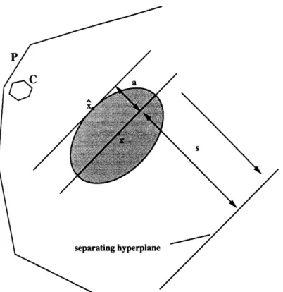
Figure 1-1: Underlying geometric representation

that the volumetric center w and the analytic center (denoted by a in Figure 1-1) will always exit. The various centers and associated Dikin ellipses are depicted in Figure 1-1 together with the convex set C and the bounding polytope P. Now, for a symmetric positive definite matrix A, we let E(A, x, r) denote the ellipsoid given by

E(A, x, r) = {y : (y- x)TA(y- x) < r2}

By Proposition A.1.1 (see Appendix) we have that P C EoUT = {x I (x - a)TG(a)(x -a) < m2}, where G(.) is the Hessian of the logarithmic barrier function associated with

P, i.e., on expanding the Dikin ellipse represented by EIN = {x I (x-a)TG(a)(x-a) <

1} C P by a factor of m we manage to contain the polytope P. The point w E P is unique in that amongst all Dikin ellipses associated with points in P, the Dikin ellipse associated with w, Ev, has maximum volume. This is easily seen from the definition of the point w that minimizes det(ATS-2A) over P. Thus, as evidenced in

Figure 1-2: Adding a constraint and moving closer to the new w

Figure 1-1, we have that,

VolEIN < VolEv < VolP < VolEoUT

Now bounding the volume of the polytope P,

1

Vol EouT = Vol E( - G, a, 1)

1 -1/2

=

Sdet [2 G(a)] < S,.mndet [G(a)]-1 / 2 < Sn.mndet [G(w)]-1 /2 _{< (2m)ne}-_V(W) (1.2) (1.3)

where S is the volume of the unit ball in Rn. It follows from (1.2) and (1.3) that

VolP < (2m)ne-V(w).

The number of planes defining P is not allowed to increase indefinitely, but is kept in check through the use of a parameter that decreases with constraint additions. This parameter which is denoted by crmin and is the smallest diagonal element of

Figure 1-3: Deleting a constraint and moving closer to the new w

the projection matrix P associated with the polytope P (see Appendix A.3 for some properties of projection matrices). Thus, the criterion employed for dropping a plane

ai is if minl<i<m ui(z) < where z is our test point and is set beforehand. An important result, im=l ai(x) = n (see A.4.1 in the Appendix), means that the number

of planes that define P never exceed n/e which implies that m = O(n). Thus if our algorithm can guarantee the long term increase of V(.) we can succeed in driving the volume of P down to zero and in so doing we can be assured of termination. So our approach will be to drive the volume of Ev to zero and this directly causes V(.) to increase indefinitely and in turn will cause the volume of P to fall.

The type of computation performed during an iteration is either one based on a constraint addition or a constraint deletion depending on the value of

t = min {ai(z)},

l<i<m

where z is the current test point.

with the separating hyperplane that the oracle returns being used as the constraint that is to be added to give the new system. If the convex set C that we use is itself a polytope, the separating hyperplane can simply be taken to be the first constraint of this set that our test point violates. This new hyperplane is 'backed off' from the test point allowing Newton steps to be taken which are complemented by line searches to move closer towards the new volumetric center.

If t < e then we delete the constraint that corresponds to the minimum ai from the constraint system that defines P, (see Figure 1-3). Since the volumetric center

w shifts as a result of a plane removal we again take Newton steps complemented by

line searches to move closer towards the new volumetric center.

1.2

Notation, assumptions and preliminaries

If x, s, or a is a vector in Rn then X, S, or E refers to the n x n diagonal matrix with diagonal entries corresponding to the components of x, s, or a. Let e be the vector of

ones, e = (1,. .. , 1). If E

cn then xlp = ixfl

p + ... + x n P refers to the p-norm

of x, where 1< p < oc; thus we have,

114X1 = Xill + * * + iX ;

Ix

1

2 = VJll2 + . . + Xn12 (Euclidean norm which we also denote by 1xl)x;

Ixllio = max{ lll, . , xnjl} (modulus of the largest component of x);

Next, for any positive semi-definite matrix B we use the notation 11j11B to de-note the proximity measure /TBf and in order to compare the positive definite-ness of matrices the following notation is used A >- () B = A - B is

posi-tive (semi) definite, with -<, defined analogously. For the matrix M we define

IM = maxAi(MT_{M) , i.e., the square root of the largest eigenvalue of the matrix}

MTM.

The Schur, or Hadamard, product of two matrices which we denote by A o B is defined by multiplying corresponding entries in the respective matrices, ie. (AoB)i = Aij x Bij and we will denote the Schur product of a matrix A with itself by A( 2) .

For x E int(P) let E(x, r) be the region

aT - bi

Z(x,r) = {y: Vi, 1<i<, iamTYb 1 - <

1 +

r} (1.4)

and note that if r < 1 then E(x, r) C P.

The volumetric barrier function V(x) is defined by V(x) = ln(det(AT S-2A)), where s(x) = Ax - b > 0, and A is an m x n matrix with linearly independent columns. Here, n refers to the dimension of the underlying space and m is the number of constraints of the system Ax > b. For a given s > 0, the projection onto the range of S- 1A (see Appendix A.3 for some properties of projection matrices) can

then be written as

P(s) = S-A(ATS- 2A)-lATs-l (1.5)

For s > 0 we then define the vector o(s) to be the vector of the diagonal entries of

P(s), ie. ai = Pii(s), i = 1,..., m. From the definition of the projection matrix P

we then have that

i = 2.aiT(ATS-2A)ai (1.6)

The gradient and Hessian of V(.) at x (see Appendix A.4) are then given by

g = g(x)= VV(x)T = -ATS-1a (1.7)

H = H(x) V2V(x) = ATS-1(3E - 2P(2))S - 1 A

Letting Q = Q(x) = ATS-2EA, then Q(x) is a good approximation to H(x), in that (see Appendix A.5)

Q(x) -< H(x) - 3Q(x) (1.8)

proximity of the iterates in the algorithm. It is defined differently in Vaidya (1989) than in Anstreicher (1994c). Vaidya denotes this quantity by (x) and defines it as the largest number A satisfying the condition that Q(x) - AG(x) and later bounds L(x) by 1/4m. However, Anstreicher defines this quantity explicitly as u(x) = (2 a/;-

-min )-1/2 after obtaining the bound shown in Lemma 2.1 in the next chapter. The

role that p(x) plays will become apparent in the subsequent chapters.

Let p = p(x) = -H-lg denote the Newton direction for V(.) at x. The new point after taking a Newton step is denoted by means of the bar (-) notation, ie. x = x +p,

= s(x), = a(s), = (x), = g(x), p = p(x), H = H(x), Q = Q(x).

To represent the constraint system after a constraint addition or a constraint deletion has occured we use the tilde () notation, e.g. S = S(x) = Ax-b, Q(x) = T,-2A,

V(x) = - ln(det(ATS 2A)), etc., to denote quantities which depend on the current point x, but are defined using the new constraint system [A, b]. On a constraint

addition the system [A, b] will be augmented to obtain the new sytem [A,b] such that

am+l ) b m+l) (1.9)

and on constraint deletions (assuming for simplicity that the mth constraint is the one to be deleted) the new reduced system is of the form [A, b], where

A = ( a ), b b (1.10)

Finally, as we progress through the algorithm we denote the sequence of iterates by xk, where k > 0 is the current iteration. Thus, we are naturally led to use the following abbreviated nomenclature: sk = s(xk), ok = a(xk), /uk _{= ,(xk), gk = g(xk),} Hk = H(xk), Qk = Q(xk). Also, at each iteration the bounded polytope that contains

C is denoted by pk and is of the form

where Ak is an Mrk x n matrix with independent columns, and bk E Rmk. Whenever we refer to the set pk, we are implicitly refering to the algebraic representation given by the constraint system [Ak, bk ], and the volumetric barrier associated with pk is the function Vk(x) = 2 n(det(Ak_{2~~~~~~~~~~~~} TS- 2Ak)), where s = Akx - bk.

Chapter 2

The volumetric barrier

In this chapter we will collect together a number of properties of the volumetric barrier function V(-) which will be used in subsequent analysis. Many of the results that will be established and the approach that will be taken relies on Anstreicher's (1994b) quadratic convergence result for Newton's method applied to V(.) for points sufficiently close to the volumetric center w (see Appendix B).

We are now in a position to analyze some of the properties of the volumetric barrier and the proximity measure

1II

1H. Let us begin by presenting the following lemma, Anstreicher (1994c), that provides a better bound on the

1II

Q measure than Vaidya (1989) achieves by explicitly working with the infinity norm IIS-AJI.

Lemma 2.1 _{Let x have s = s(x) > 0, and let a = a(s). Then V E in,}

(TQ~ > (2V _ min ) S-1A 12

Proof: Applying the same technique as in the proof of Theorem A.5.2 (see Appendix) and using the same change of variables, proving the lemma is equivalent to proving that

'T

_U3uT

_{(2/' mi} n

- min)U (2.1)

the problem m min u1 2 + 'mi nj (T )2 i=2 (2.2) m s.t. E (uT)2 = j112 -1 :=2

the solution value of which is obviously llu 112 + min( 112 - 1). Since 1 = lulT <

~u111

llU

Ž1l

l/

2

.

Letting

-2

0 = j1f112

>Fl

>

1,

the

solution value in (2.2) is therefore no lower than the solution value in the minimization problem

in min( 1) } (2.3)

0>1 0 -min- -1

A straightforward calculation shows that the solution in (2.3) is 0 = 1/a,, with objective value 2a-min - rmin, proving (2.1) and the lemma.

Let us define / = (x) = (2 -min - 'amin)- 1/2* Then Lemma 2.1 and (1.8) imply

that

6 = IIS-1Aplo, < IIpllQ <

llpIIIIH

(2.4) There are two quantities that the algorithm will need to maintain explicit control

over, namely the measure llPllH and the quantity

PllIpllH

and they will later be used to

argue that following a constraint addition or deletion only a small number of Newton steps suffice to return the current iterate to a suitable proximity of w. The results of the following lemma follow from the quadratic convergence result, namely Theorem B.7 (see Appendix) and (2.4). It establishes quadratic convergence properties written entirely in terms of the measures we seek control over, in addition to a relationship between Q and Q that will be needed in the proof of Theorem 2.4.

Lemma 2.2 Let x have s = s(x) > 0. Assume that

IIlpllH

< .014, and let = x + p. Then

ii) HfllpIH < 21.6/1 plH,

iii) Q < exp(6.02/ulpllH)Q

Proof: Using Theorem B.7, (2.4) and the fact that IJpjjQ <

flPH,

we get that

19/t(1 + /I1PH) )

t/~ f < (1 - lplH)6 H < 21.27 Hp (2.5)

where the last inequality uses the assumption that jllpIH < .014 = i) holds true. Next, since 6 < 1 E E(x, 6) C E(x, [uljPIIH) and it follows from Proposition B.3 that

(2.6)

(1 + 6)2 - - (1 - )2

(1 +) 2 - ai - (1-) 2

and this gives us that min > min(l - 6)2/(1 + 6)2. Since the function 2x/ - -y is

monotone increasing for y E [0, 1], it follows that

2Vmin - min 2 '( 1 - A

1 + 6

- 1 _n( 6 2

- 1'i + 6) > (2/om - umin)

and therefore t = /(z) = (2v/oi=-nmin)- 1 /2 < (1+ 6\1/2

" k1

- 61 1 + plPH 1/2 z1 -PH)

where the last inequality uses (2.4). Substituting /LHP IH .014 into (2.8), and combining the resulting bound with (2.5), proves part ii).

Proposition B.3 and (B.1) we get that

OTQ < (1 + )4

Next from combining

V E Rn, and therefore

6)

- 2 ln(1 - 6) (2.9)

But for 0 < 6 < 1, ln(1+6) < 6, and ln(1-6) > -6-.562/(1-6) = -6[1+.56/(1-6)] 1+61+ (2.7)

(2.8)

Combining these facts with (2.9), and using IlPIIH < .014, we obtain

in

(,-)

<

4

p||H

+ 2

2L + + 2(1- 014

)

< 6.02/ lP H

E7TW

+2(1(-.014)

proving iii). o

Lemma 2.3 Let P = {x I Ax > b}, where the columns of A are independent, and assume that the interior of P is nonempty. Then p is bounded V(.) attains its minimum at a unique point w of P.

Proof: If P is bounded then V(.) clearly attains its minimum over P at a unique interior point, since V(-) is strictly convex in the interior of 7P, and V(x) - o as x approaches a boundary point of P. Now assume that P is not bounded, hence P must contain a ray, say r, such that if x E P then x' = x + Or E P for all 0 > 0.

Letting s(O) = A(x + Ow) -b = s + Aw > 0 (since Aw > 0, Aw $ 0) and using

aiaiT

the fact that ATS(O)-2_{A = ( ai)} 2 _{on letting - o, we see that the} (s +aTw)2

matrix ATS()-2A tends to become more and more like that of a Null matrix =>

det(AT_{S(O)-2A) - 0 V(x') - -oo and therefore no minimizer w can exist.}

Theorem 2.4 Let x have s = s(x) > 0, and assume that /lIpIIH < .014. Then V(.) has a unique minimizer w E int(P), and V(x) - V(w) < 1.11Ipi2.

Proof: Consider an infinite sequence of Newton steps initiated at x° = x,

xk+l = xk + pk for k > 0. Applying Lemma 2.2,

/Pllpt][H1 < 21-6(/ 011p llHO) < 21.6(.014)2 _{< .014}

and by induction it follows that kllpklHk < .014 for all k > 0. Lemma 2.4 then implies

IIPk+lllHk+l

< 21.6plIpk 11k < 21.6(.014)[lpkllHk < .3111Pk lIH (2.10) forall k > 0, and therfore llpklHk - 0. Also, since V(.) is strictly convex, the

subgradient inequality implies that

V(Xk+l) > V(Xk) + gkTpk = V(Xk) _ Ipk 2k

If it is the case that xk - w E int(P). Then H(w) being positive definite, (2.10)

implies that g(w) = 0, and therefore w is the unique minimizer of V(-). Moreover, using (2.10) and (2.11) we have

V(w) 00 = V(xo) + [v(Xk+l) _ V(X)] k=0 00 > V(x) - _k=OE (097)pk > V(x °) - (1.10971)jjIIp k=O > V(X ) _ 1.111p0 12HO (2.12)

as claimed in the lemma. To complete the proof we must prove that the sequence {xk) converges to a point w E int(P) and to bound the sequence we will first prove

that

Q = QO < 1.14 Qk (2.13)

for all k > 0. Now, since

T_QOJ TQkq k-1

=

j=0 (2.14) OVQjl ~TV+1l

and part iii) of Lemma 2.2 implies that

(In TTQO k-i

=o

j=0 TQjk MTj+l ( k-1 < E 6.02,jllP pHj j=O (2.15)

and through repeated application of part ii) of Lemma 2.2 we get

Hj

IpJIIHj

< (21.6)2 -1(L0 p°lHO)2

,

(2.11)

Substituting (2.16) into (2.15), using p°llpllHo < .014, gives us

In

(

Q)

< 6.02 k-1Z(21.6)2 J-1 (P0f°lp° 0 Ho)i 2 j=O 602 2 0- (21.6

_oIHo)

0_LO

_p

0 2_J 21.06 3=0 < .28 (.31)ij l j=o .28(.31) 1 - .31

Exponentiating (2.17) proves (2.13). Using (2.13), (1.8) and (2.10) we then have that xk _X OIIQ k-1

< E IIx

j +l

_{- XjQ}

j=O k-1

< V.14

Ip

IIHj

j=o <

1.14-(.31)

°jIp IHo j=0o < 1.5511p°llHo (2.18)

But from Lemma 2.1, IIS-1_{AIloo < / IIQ V~. Letting = x}k that

- x° , (2.18) implies

IS-lA(xk -

x

°

_)Io

_<

_{1.5511P°llHO}

_<

_.022 and therefore

sk

.978 < - < 1.022,

0

-S. k > 0

From (2.18) we get that

IIxkQll

< IIxOIIQ + 1.551poIIHo and since Q =

(2.19)

RTDR

>-Amin = l1xk < 1j IXkII,2 we get that the entire sequence {xk}

- Xmi_n Q is bounded and

from (2.19) the sequence lies in the interior of p. By the Bolzano Weirstrass theorem (2.17)

there exists at least one accumulation point and it is an interior point of P. Then

pkIHk -+ 0, from (2.10) implies that g(w) = 0 at any accumulation point w of {(k}.

But there can only be one such point, the minimizer w of V(.), and therefore xk - w

Chapter 3

The algorithm and its complexity

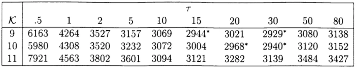
In this chapter we will present the cutting plane algorithm. The original version of this algorithm was first developed in Vaidya (1989), later went through some changes in Anstreicher (1994c). These changes were mainly improvements in the definitions of some key parameters and the use of the Hessian of V(.) in the computation of the Newton steps, the effect of which was a dramatic reduction in both the number of Newton steps required for termination and the maximum number of constraints used to define P. We further introduce a linesearch into the algorithm following each Newton step that brings in an additional parameter, namely the number of steps taken in the Bisection Method [1] that we have used in performing the linesearch and that we denote by KIC. The performance of the algorithm and the efficacy of the linesearch is measured by the total number of inversions carried out until termination. The values assigned to our parameters was done in such a way so as to minimize the number of inversions carried out by the algorithm and this is discussed in Chapter 5.

3.1

The volumetric cutting plane algorithm

The Bisection Method [1] is used with termination after KC bisections. Given the current point x and the Newton direction p the problem

min f(c) = V(x') = V(x + oap)

where c is the step-length and x' will be the next current point, has a unique solution since the function V(.) is strictly convex. The quantity ma.x is the value that will

take x' to the boundary of the polytope P and is computed using the min-ratio test, namely

Si mnin

l<i<m aTp

s.t. aTp < 0

The Bisection Method [1] uses a gradient function and a closed step-length range. In our case a simple differentiation with the aid of the chain rule yields

f(a) = -cTS(c)-lAp

We now present the pseudo-code of the cutting plane algorithm with a linesearch following every Newton step.

Step 0. Given x°, P ° = {xlA°x > b°}, 0 < < 1, Y > 0, 2 > 0, L, KC and Vka.

Go to Step 1.

Step 1. If Vk(xk) > Vkax, then STOP. Else go to Step 2. Step 2. If ak > E, go to Step 3. Else go to Step 4.

Step 3. (Constraint Addition) Call the oracle to see if k E C. If so, STOP.

Other-wise the oracle returns a vector ak E Rn such that akTx > akTxk Vx E C. Let [Ak+1, bk+l] be an augmented constraint system having ak+

1l = ak, bk+l < ak k. Go to Step 5.

Step 4. (Constraint Deletion) Suppose that jk = akin < E. Let [Ak+l, bk+l ] be the

reduced system obtained by removing the jth contraint. Go to Step 5.

Step 5. (Newton Direction) Let ° _{= k. Compute the Newton direction and take a} sequence of steps with the opitmal step-length a of the form ij+l = ij + ajii, where

p

= p(ij), j > 0 (go to Step 6 at each iteration) until pJjJ < y1,

PfJIIP Jlfj < Y2, where HJ = H( J), i = - p(). Let xk+l = J, set k = k + 1,

and go to Step 1.

Step 6. (Linesearch) Initialize amin to 0 and ma,, to minl<i<m - si/aTp s.t. aTp < 0. Then, For i = I to KC Do: a = (amin + amax)/2. If f'(a) < 0 then min = a.

Else ama,, is set to a, End. Go back to Step 5.

In Step 3 the value of bMk+I that corresponds to the placement of the new con-straint is not arbitrary, but will be prescribed precisely in terms of a parameter r > 0

in Chapter 4. Also, throughout the algorithm the iterates xk will have IIpkllHk < 'l,

Pk pkIpk < y2 for all k.

3.2

Initialization

In Step 0, the initial system is taken to be

po = {x En Ilx _> _ 2_{L,j = 1,.. ,n,eTx < n2L}}

Note that P0 then contains a sphere of radius 2L, centered at the origin. What is the volumetric center of P0? It is the point x such that ATS-lr = 0. To simplify matters in calculating this point it will suffice to consider the scaled system 50 given by

po = {x E n I xj > -,j = 1, .. ,n,eTx < n}

since if x E P° then x/2L E p°o, and so the volumetric center of P° will simply be 2L times the volumetric center of P5. Proceeding therefore with

Si = xi + si = -eTx + n we get that ATS-1 = 1 x₁+l O 1r = 1 eTi Xn+ 1 eT-n/ ?_A + n+1 x₁+1 eTx-n axn + n+1 \Xn+l eTx-nl

and so our point x that will be our volumetric center must have the following property

(xj + )n+l

eTx - n (3.4)

Now, using (1.6), (3.1) and (3.2) we have

(ATS-

2

_A)

- 1

cTi = (Xj + 1)2 eT(ATS-2A)-le

(Xj + 1)2

and together with

(ATS-2A)-1 =

(x1 + 1)2

0 _{(Xn + 1)}

where wT = ((x1 + 1)2, ... , (Xn + 1)2) , we get that

(xj + 1)2[i(xi + 1)2 + (iX i - n)2 - (Xj + 1)2]

j = 1, *,n (3.6)

(EiXi - n) 2Ei(Xi + 1)2

i(x _i + 1)2 + (ixi - n)2 (3.7)

from (3.6) and (3.7) we find that (3.4) is satisfied if Eixi + xj = n - l, j = 1,., n,

ie. for Dx = (n - 1)e, where D = I + eeT, a straightforward calculation using the and l<i<n i = n+1 (3.2) =0 _(3.3) wwT (eTx - n)2 + Ei(xi + 1)2 Oj = (3.5) and

n-1

Sherman-Morrison-Woodbury formula A.2.1 gives us that xi = n+l' i = 1, n. This is a strictly interior point of 'P0 and is therefore the unique minimizer, i.e., the volumetric center. It is also interesting to note that the analytic center for P° happens to coincide with the volumetric center for this case.

It can easily be shown through induction that the determinant of a matrix D of the form D = c + deer, where I is the identity matrix is given by det(D) = cn-l(nd + c). In computing V(x), it can be seen from (3.1) and (3.2) that the

matrix G°(x°) will be of this form and a straightforward computation gives us that ( n+1 \2n

det(G°) = rn2L+1 (n + 1) and so the value of V0(.) at x° is

V°(x°) = -ln(2)n(L + 1) + nln(1 / + + In(n + 1) > -. 7n(L + 1) n) (3.8)

3.3

Termination

The value of Via > 0 which depends on mk and that is set in Lemma 3.3.1 is such that Vk(xk) > Vkax implies that Vol (pk), and hence also C C pk, is less than that of an n dimensional ball of radius 2-L. However, since from the outset we have assumed that if C is non-empty then it must contain a ball of radius 2-L, this result would mean that the convex set C is empty. Note that by construction, from Step 5 of the algorithm, all of the iterates will satisfy flpkllHk < l, L/kllPkIIHk < 72.

Lemma 3.3.1 Assume that the iterates of the volumetric cutting plane algorithm satisfy lIpk IHk < .014 forall k. Then on setting Vkax = .7nL + nln(mk) termination in Step 1 establishes that Vol (C) is less than that of an n dimensional sphere of radius

2-L

Proof: By Lemma 2.3 and Theorem 2.4, pk is bounded for each k, and therefore the analytic and volumetric centers of pk both exit. From (1.2) and (1.3) we have

that

Vol(9Pk) < Snme-Vk(k) _(3.9)

and since C C pk Vk > 0 to show that Vol (C) is less than that of an n dimensional

ball of radius 2-L it suffices from (3.9) to have

Snmkne- Vk(wk) < S2-nL

and on taking logarithms this is equivalent to

Vk(wk) > nLln(2) + nln(mk) (3.10)

But Theorem 2.4 and ]IpkllHk < .014 imply that

Vk(wk) > V(x) - .00022

and so (3.10) is satisfied if Vk(xk) > .7nL + n ln(mk). [

3.4

Complexity

Assuming for a fixed c > 0, and 7Y2 < .014 the algorithm achieves

Vk+l(xk+l) Vk(xk) + AV+ (3.11)

on steps where a constraint is added, where ZAV + > 0, while on steps where a con-straint is deleted it achieves

where AV- > 0. From the boundedness property of pk and noting that P0 is defined by the least number of constraints needed to bound a polytope in ~R it is apparent that at any point in our algorithm we will have that the number of constraint additions that have occurred will be greater than the number of constraint deletions. Thus, if we can guarantee that AV = AV+ - AV- > 0, then as the next theorem shows our algorithm will terminate in (nL) iterations.

Theorem 3.4.1 Assume that the iterates of the volumetric cutting plane al-gorithm, using > 0, 2 < .014, satisfy (3.11) and (3.12) on iterations where a constraint is added or deleted, respectively. Assume further that AV = AV+ - AV-is Q(1) and positive, and that the number of Newton steps in Step 5 of the algorithm is 0(1). Then using Vmka, as in Lemma 3.3.1, the algorithm terminates in 0(nL) iterations, using a total of O(nLT + n4L) operations, where T is the cost of a call to

the separation oracle.

Proof: The number of constraint additions being greater than the number of constraint deletions, together with (3.11) and (3.12), implies that

Vk(xk) > V(x °) + k(AV+ - AV-)/2 = V°(x) + kAV/2 (3.13)

Next, the fact that on steps where a constraint is added we always have kin > , and mkain < eTak = n for all k, implies that mk < (1/e)n + 1 < (1 + 1/e)n for all k. Using this fact with (3.8) and (3.13), we see that Vk(xk) > Vk certainly occurs if

-. 7n(L + 1) + kAV/2 > .7nL + n ln( + 1/e) + nln(n)

and therefore the algorithm must terminate for

2n(1.4L + ln(n) + ln(1 + 1/e) + .7)

k > AV = 0(nL) (3.14)

AV

Finally, noting that mk < n(l + l/e), we have that the work per iteration for the algorithm using standard linear algebra is O(n3 ) and as a result the total complexity

of the algorithm is O((nLT + n4L) operations, where T is the cost of a call to the

Chapter 4

Adding and deleting constraints

Results will be proved that characterize the effects of constraint additions and dele-tions, that occur in Steps 3 and 4 of our algorithm, on V(.), a, and IIPIIH, respectively. We will see that from the observations following Lemma 4.1.1 and Lemma 4.2.1 we will have that AV = - V- = ln(l +Tr)/ 2-ln(1-e) - 1/ 2_{, where the quantity r is}

yet to be defined. We will leave the analysis of the Newton steps and linesearches that occur immediately after a constraint addition or deletion to the following chapter.

4.1

Constraint additions

We now consider in detail the effect of adding a constraint in Step 3 of the algorithm. Dropping all dependence on the iteration k to reduce the burden of notation, and with our new system defined by (1.9) with the assumption that aT+1x > bm+,, so

that sm+1 = aTm+lX-bm+ > O we let

r = +laT (ATS-2A) am+1 (4.1)

2

separating hyperplane

Figure 4-1: Setting the value of r

the following program:

Max a+(x - )

s.t. (x - )TATS-2A(x - ) < 1

we have that the solution occurs at x (see Figure 4-1) with maximum objective function value given by

a= amaT+(ATS-2A)-lam+l

and so T = (o/Sm+1)2

From a geometric perspective = (a/s)2 is the ratio of the distances a and s squared as can be seen in Figure 4-1, and so decreasing 7 has the effect of pushing the separating hyperplane ever further away. It is advantageous to have the separating hyperplane as close to the test point as possible, as this will result in the greatest decrease in the volume of the polytope P on the next iteration and hence the greatest

increase in the function V(.) and that is what we hope to achieve. Thus, it will be attempted to set T at a maximum value in such a way as to still be able to satisfy the assumptions of our theorems in Chapter 2 that prove convergence of the algorithm. The quantity T being set beforehand in this way, will necessitate computation of the value s,+l during each iteration in order to satisfy (4.1).

We will now prove three results that demonstrate the effect of a constraint addition on V(.), , and llPllH, respectively.

Lemma 4.1.1 Suppose that a constraint (a T±, bm+l) is added, and T is given as in (4.1). Then V(x) = V(x) + 1/2 ln(1 + r)

Proof By definition,

V(x) = in [det (ATS-2A)]

2 1)]

-2 ln[det(ATS-2A + sm+am+laT+)]

- [det ((ATSA) (I + (ATS A)-lam+la ))]

V(x) + ln[det(I + sm2 l(ATS 2A)-1_amaT)]

The lemma then follows from the definition of T, and the fact that det(I + uvT) = 1 + uTv.

Note that from the above lemma we have that following a constraint addition

V(w) - V(w5) > ln(1 + T)1/2 and thus in Theorem 3.4.1 AV+ will be represented by ln(1 + )1/2

Lemma 4.1.2 Suppose that a constraint (aT+1, bm+l) is added, and r is given as in (4.1). Then &m+1 = T/(1 + T), and ai > i > ai/(1 + r), i= 1,...,m.

Proof We have that ATS-2A = ATS-2A + s2+lam+laT,+, so the Sherman

-Morrison-Woodbury formula A.2.1 obtains

(AT'SA=-A2A )- T 2A 1- - _{(AAT TS A)-2A-lam+la}T_{+ (ATS-2A)- (4.2)}

Now i = _{Now~i Si} s-2aiT(ATS-2A)-lai, ₆₁ so from (4.2) we immediately obtain,

5i = Oi

-8-2 -2 /(aT(ATS-2A)-a,,1+)2

1, -47- , z 1,...,m

I+T7

Note that (4.3) implies that ai > ai, i = 1,..., m. Applying Proposition A.2.6

Is-1 -1 T(ATS-2A)lam+ _{< lIsi-ail (ATS-2A)-1 HlSIliam+ll (ATS-2A)-'}

Combining (4.3) and (4.4) then obtains 3i > rir/( + T), i = 1,...,m, which is

exactly the bound of the lemma. Finally, from (4.2) we have

&m+l = Sm-+lam+1(A S A) aml = 1+ *

Theorem 4.1.3 Suppose that a constraint (aTm+l, bm+ ) is added, min > e > 0, and r is given as in (4.1). Then

ipiHf

< V'-

(

1IPII

H

+

T(1 + FT1) 1 + T l+T

Proof Using Lemma 4.1.2, we have

m+l Q =

:

-aiaiT i=1 z 1 1 +T aOi T 2 aiai i=1 i 1 =

Q

1+T

and therefore Q-' - (1 + r)Q-1, by Claim B.2. As a result,

lIIPI h I=II-ft' < I|9| |-1 < + Tjj1Q- 1 - 1 +l AT-IaJlQ -1

where the first inequality uses (1.8) and Claim B.2. We also have that

m+l i ATS-a& = E i ai i=l Si m di = --ai i=1 Si a-m Um+l +Eai 's a,+l i=1 Si Sm+l (4.3) (4.4) (4.5) (4.6)

= vaI

Since g = ATS-1a, combining (4.5) and (4.6), and using the triangle inequality, obtains iPHl < 1I T (9HQ-1

+

fI

E

ai

IIQ-1

i=1 Si + 'm+lam+l Q- 1 Sm+1

Next, from (4.3) we have

11

- aiai 12 -1 = dTEl/2S-lA(ATS-2EA)-lATS- 1E/ 2d <

i=1 i

where

lldl 2 (4.8) -2 -2 (a (AT S-2A)-a +1)2

a1/2(1 + T)

and the last inequality follows from the properties of projection matrices (see Ap-pendix A.3).

Using the bound from (4.4), we have Idil< ra/2/(1 1 + r), i = 1,. . , m, so

m

i=1

< m s_{i sm+lam+(ATS-}2 2_{A)-laiaT(ATS-}2_{A)-lam+ T1/2}

i=l 1/(1 + ) 1 + T

-2 T 2

T(1 )22a+ m+ m+am+l

(4.9) (1 + r)2

Combining (4.8) and (4.9) then obtains

HE

i=1 ai IIQ-1 si T -1+r (4.10)

The fact that amin > = Q = ATS-2A >- eATS-2A, giving us that Q-1 < (1/e)(ATS- 2A)- 1, and as a result,

m+1 2

-1

< E-&+2 S a +1(A S -2A) -lam+l

II amm+ IQ O1m+l m+la+

$m+l

T T2

e (1 + )2 (4.11)

where the last inequality uses m,,+l = r/(1 + r), from Lemma 4.1.1. Finally, using

Q-1 < 3H-1 from (1.8) and Claim B.2 we get

flgIlQ-1 < v g11IgjH-' = V |pllH _(4.12)

The proof is completed by combining (4.7), (4.10), (4.11) and (4.12). a

4.2

Constraint deletions

We now consider the effect of deleting a constraint, as occurs in Step 4 of the al-gorithm. We again drop all dependence on the iteration k to simplify notation and simply consider the system given by (1.10), where once again for simplicity we assume without loss of generality that the mth constraint is the one to be deleted. Assum-ing that the columns of A are linearly independent then linear independence of the columns of A is a consequence of am < < 1, as will be seen from (4.13), where for

am in that range we get that (ATS-2A)-1 _{is positive definite , ATS-2A is positive} definite and thus the columns of A must be independent. This is an important obser-vation as the proof of the boundedness of pk _{deduced from Lemma 2.3 and Theorem}

2.4, requires that the columns of Ak be linearly independent for all k.

We now proceed to establish the three results (as in the case for constraint addi-tions) to show the effect of a constraint deletion on V(.), , and IIPIIH, respectively. For the latter, we give a result in terms of amin, and not > min, for reasons that will become clear in the next chapter.

Lemma 4.2.1 _{Suppose that the constraint (a , bin) is deleted, where am < e.}

Then V(x) > V(x) + 1/2 In(1 - ).

Proof By definition,

V(X) = ln[det(ATS-2 A)]

= ln[det((ATS-2A)(I- s2(ATS-2A)-lamaT))]

= V(x) + ln[det(I- ½ s2(ATS-2A)-lama)]

The lemma then follows from a, < E, and the fact that det(I - uvT) = 1- uv. a

It is worth noting that from Lemma 4.2.1 we can establish that 0 < V(tw)- V(wh) =

ln(1 - a,) -1/2 < ln(1 - e)-1/2 and thus in Theorem 3.4.1 AV- will be represented by

ln(1 - e)- 1/ 2.

Lemma 4.2.2 Suppose that the constraint (aT , b ) is deleted, where am < e. Then ai < ji < ai/(1 - ), i = 1 ,..., m- 1.

Proof We have that ATS-2A = ATS-2A -s 2 amaT, so the Sherman -

Morrison-Woodbury formula A.2.1 obtains

(ATS-2A)- _{= (ATS} - 2 A ) - ₊ s(2 (ATS-2A)-laI aT (ATS-_{l m} 2A)-l

1 - am (4.13)

Now i = s-_{Nowai= i} 2aT(ATS-_Ii\ 2A)-lai, so from (4.13) we immediately obtain,

= + s Sm (a_i (A T A) am)

1 - am

(4.14)

Note that (4.14) implies that ai ai, i = 1,...,m - 1. Applying Proposition A.2.6 as in (4.4), then obtains

Ils-1 s aT(ATS-2A)-lamI < _{1i m ai}ajm (4.15)

Combining (4.14) and (4.15) and using am < , then obtains ai < ai + aie/(1 - e),

i = 1,..., m- 1, which is exactly the bound of the lemma.

Theorem 4.2.3 Suppose that the constraint (aT, bm ) is deleted, where am = amin. Then

Proof Using Lemma 4.2.2, we have

m-1

i(i T j=1 Si

m

ai T m T am T

E aia - 2amam =

Q

- -ama,

i=l S m m

Using Claim B.2, and the Sherman-Morrison-Woodbury formula A.2.1, we then have

- 1_{_l (Q}

'm

m

msQ-2ama TQ-1

1 - mSm amQ am

Since we know that Q = ATS-2AEA aminATS-2A, Claim B.2 implies that Q-1 <

(1/Omin)(ATS-2A)-1, and therefore

Sm2aTQ- lam < 1 -2aT (ATS-2A)-lam - m

min rmin

Combining (4.17) and (4.18), and using am = amin, then produces

Q-1 _ Q-1 + min m2Q - T -1 - iSm ama - ~1 -Omin 1 (4.18) (4.19) and therefore I1II = 1-₁ <

-I

₁ < 19|2 1 -+ Omin 1 - min

(

T _Q-la m\ 2 Sm

where the first inequality uses (1.8)'and Claim B.2. Next from Proposition A.2.6 we have

(4.21)

where the last inequality uses (4.18). Combining (4.20) and (4.21) then obtains

I[Ip2I < II2-1 + 1min -I = lll- (4.22)

H- - min 1 1 - min

(4.17)

(4.20)

Now

m-1 m m m-1

i-g = AT&S-7 =

S

-ai = E i ai +E i- oi

i=l Si i= Si i=1 Si

so (4.22) and the triangle inequality imply that

IIPII

<

I

(II9IIQ-1

+ L- Ei ai a Q-1

t=1 Si

+ 1-am IQ-i

Sm

Next, from (4.14) we have

m--1

II

- ailQ_ = dTZl/2S-IA(ATS-2ZA)-'ATS- l l/2d <

lld

2 i=1 Si where di = (4.24) 2i S2(aT (ATS-2A)-'am)2 1/2(1 - Um) Ol ( - .

and dm = 0, with the last inequality following from the properties of projection

matrices (see Appendix A.3).

Using the bound from (4.15), and the fact that am = umin, and also noting that

dil < a1/2Omin/(1 - Omin), = 1, ... , m - 1, we have

m

i=1

< rn-i _sim s-2 -2- T ATS-2A)-aaT/ ATc-2A-1 _{1/2 1a-- ina} 1/2

zi=l - 7i (I- min) 1- min

s

~smam(ATS2

A) laiaT(ATS_i 2 A)-la '

'~ 8i2-2aT(A T A)-laia(A TS-2A)-lam o2

Ui/ (1 1 - Umin) Umin -2 TT (1 - min)2 m am A S 2 A) am 2 U-min (1 - Umin)2

Combining (4.24) and (4.25) then obtains

11 -Si i Q-1 i=l i 1 - 'min (4.25) < min 1 - O'min (4.26) Om -am (4.23) <

Finally, using (4.18),

-IIam Q-l m a = m = 'i < in (4.27)

Sm -1 - min

Chapter 5

Analysis

In seeking to find the maximum number of Newton steps that would guarantee the next iterate satisfies the proximity conditions we will use the more general results

pf -11 19(1 + Hll pH) 2 (5.1)

and

IPit 1-9 (< 1 IpIIH)2.5 (HIIP1 H)2 (5.2) which follows from the analysis used in the proofs of parts i) and ii) of Lemma 2.2.

There are four parameters that will play a role in the analysis, namely r, , 'Yi and 7₂. Intuition tells us that it is wise to set r large; however, we are restricted by

the bounds in Theorem 4.1.3 and Theorem 4.2.3 on the proximity measure 11l511I that must be maintained for all the iterates in a run of the algorithm. These bounds play an important role in establishing that the number of Newton steps that are needed to recover the proximity conditions after a constraint addition or deletion is 0(1) and this is required by the convergence Theorem 3.4.1. In order to set r at an optimum value and still satisfy the bounds the following parameter settings were used: was set to .0062, = .0049, yl = .000006 and y2 = .0001. With these settings, the maximum number of Newton steps on a constraint addition was shown to be 7, while

the maximum number of Newton steps on a constraint deletion was shown to be 4. These results are established in the following two theorems.

Theorem 5.1 Let x be a point with s = s(x) > 0. Assume that Yl < .000006,

and 72 < .0001 . With amin > = .00475 and with 7 set to .0062 suppose that a

constraint (am+l, bm+l) is added, and let [A, b] be the augmented constraint system. Let x be obtained by taking 7 Newton steps for V(.) starting at x. Then

i) IIPIIH < .000006,

ii) f

IPI

<

.o0001,

iii) V(z) > V(x) + .0025438

Proof: Since 'min > E, and 7- > , Lemma 4.1.2 implies that &min > /(1 + 7) >

.00472 and therefore

(5.3)

- = (2 min - min) 1/2 < (2 .00472 - .00472)1/2 < 2.745

Also, Theorem 4.1.3, with 7 = .0062, gives

iPjH 1.0062

(v(.000006)

+ .0062(1 + 1.0062 ) < .01325 (5.4)

Combining (5.3) and (5.4) ,

tI11pf

< 2.745(.01325) < .0364. Using the same notation as in Step 5 of the algorithm, repeatedly applying (5.1) and (5.2) then obtains

IIPIIH

lip7

IIf

t1~411~

< .012290, < .010837, < .008514, < .005165, < .001803, < .000205, < .000003, -211p2 I2 I _ 3113 11f_ F511 5 l f11J

711

7

11a7

< .034989 < .031952 < .025916 < .016137 < .005724 < .000655 < .000008

proving parts i) and ii). The proof of part iii) follows from repeated application of the convexity property of V(.), namely if x = x+ then V(x) > V(x)+gT = V(x)- t32 .

Using this convexity property and Lemma 4.1.1 we have

6

V(X)

>

V(x) + ln(1 + T) -

PS

I/lJ

j=o

= V(x) + .5ln(1.0062) - (.013252 + .012292 + ... + .000212)

= (x)+ .0025438

proving part iii) and the theorem. [

We now consider the case where a constraint is deleted.

Theorem 5.2 Let x be a point with s = s(x) > 0. Assume that 7Y1 < .000006,

Y2 < .0001 and that am = amin < e = .00475. Suppose that the constraint (am, bin) is deleted, and let [A, b] be the reduced constraint system. Let x be obtained by taking 4 Newton steps for V(.) starting at x. Then

i) 11p1lH < .000006, ii) fI p a < .0001,

iii) V(x) > V(x) - .0025125

Proof: By Theorem 4.2.3, using am < E,

ft(Hft

1 ( + .0095

i.p99525 < .99525/

Also, by Lemma 4.2.2, min > min, and therefore <

again, using armin < e, and IIH < .0001, then obtains

< .009579 /p. Applying Theorem 4.2.3

1\/

(V'IIPIIH + I

)

1 (.000173+ 2 minl ) 9952 .99525. < .0001 7 36 + 2_{.0140min (5.5)}

But Jmin < = .00475, so min < V /-Vmi;j = .0689 amin and therefore

= (2 - min)'/2 (1.931 / ;)2- 2 < .7197ami (5.6)

Combining (5.5) and (5.6) and using min < e = .00475 we then have that

/fJijpjf < .0001736 + 2.014(.7197)(.00475)3 / 4

< .00264

Using the same notation as in Step 5 of the algorithm, repeatedly applying (5.1) and (5.2) then obtains < .005943, < .002174, < .000272, < .000004,

11

IP'1jf1

< .016819

flIP2fl

_I

2

_{< .006257}

f3P311f3 1 < .000787 /4 11p4 I4 < .000012 proving parts i) property of V(.) and ii). To and Lemma

prove part iii) we again repeatedly use the convexity 4.2.1 to give us 3 V(X) V(x) + ln(1 - e) -Z

IlpJi

j=o > V(x) + .51n(.99525) - (.0095792 + 0.0059432 +... + .0000042) • V(x) - .00251

proving part iii) and the theorem.

From Theorem 5.1 and Theorem 5.2 we see that AV = AV+ - _{AV- = .0025438} -.0025125 = .000031 > 0. It is not possible to increase r much further and still satisfy the proximity conditions. Insignificant increases in beyond this value merely increases the number of Newton steps that will be needed after a constraint addition or deletion and also results in a huge decrease in V. Further increases in r merely results in AzV becoming negative and thus violating the assumptions of Theorem 3.4.1.

ll

1 13

I

5.1

Comparison with Anstreicher's and Vaidya's

constants

In terms of specification of the algorithm, this algorithm differs from Anstreicher's algorithm in that we have included a linesearch prior to every Newton step and have used a different set of parameters. As for Vaidya's algorithm it takes Newton steps based on directions d = -Q-g and uses a proximity measure based on V(x) - V(w),

where w is the true minimizer of V(.). By contrast the fundamental proximity mea-sure used here is [IP[H, but explicit control over the meamea-sure [llplH is also necessary. Anstreicher's quadratic convergence result gives much sharper control over the prox-imity measures, using Newton steps, than Vaidya has over his measure V(x) - V(w) and this means that r and can be increased on steps with constraint addition and deletion while still returning the proximity measures to their prescribed values using a very small number of Newton steps. This is obviously very desirable from a practical perspective and is what motivated us to find how large we can increase r and still be able to establish the same complexity result.

Now, a larger e means that we will carry fewer constraints (the maximum number of constraints carried being n/e+ 1), and in practice a larger setting of r translates into an immediate larger value for AV that will lead to fewer iterations of the algorithm. In his analysis Vaidya uses e = 10- 7 _{and his AV is about 1.325 x 10}- 7_{. Furthermore,} on a step where a constraint is added Vaidya's algorithm takes 2197 Newton-like steps (based on the matrix Q), while on a step where a constraint is deleted his algorithm takes 1493 Newton-like steps. Anstreicher sets T = .0035 and e = .0025, in one of the instances that he considers, resulting in AV = .00033 with a total of 3 Newton steps taken on an a constraint addition and 2 on a constraint deletion. In our attempt to set T at a maximum value, while still satisfying the requirements of the convergence Theorem 3.4.1, we get that r can be increased to .0062 (an increase of more that 77% over Anstreicher's setting of r) with = .0049, ?lY = .000006 and y2 = .0001 and this gives zAV = .000031 with 7 Newton steps taken on a constraint addition and 4 on a constraint deletion. The restrictions imposed by the proximity measures and the