HAL Id: hal-02792512
https://hal.inrae.fr/hal-02792512
Submitted on 5 Jun 2020HAL is a multi-disciplinary open access archive for the deposit and dissemination of sci-entific research documents, whether they are pub-lished or not. The documents may come from teaching and research institutions in France or abroad, or from public or private research centers.
L’archive ouverte pluridisciplinaire HAL, est destinée au dépôt et à la diffusion de documents scientifiques de niveau recherche, publiés ou non, émanant des établissements d’enseignement et de recherche français ou étrangers, des laboratoires publics ou privés.
A practical method of global sensitivity analysis under
constraints
Jean-Pierre Gauchi
To cite this version:
Jean-Pierre Gauchi. A practical method of global sensitivity analysis under constraints. [Technical Report] 2015-1, 2015. �hal-02792512�
A practical method of global sensitivity analysis
under constraints
Jean-Pierre GAUCHI
Technical Report 2015-1, february 2015
UR1404 MaIAGE
Mathématiques et Informatique Appliquées du Génome à l’Environnement INRA Domaine de Vilvert 78352 Jouy-en-Josas Cedex France http://maiage.jouy.inra.fr © 2015 INRA
Jean-Pierre GAUCHI
Abstract
A novel practical method to conduct a Global Sensitivity Analysis (GSA) for computer models is proposed in this article. It is based on Partial Least Squares polynomial regression metamodeling, used in conjunction with a D-optimal computer experiment design. This practical method is particularly well adapted to the following four situations: (i) when the cost of a single computer simulation run is very high (long computing time), limiting computation to just hundreds of simulation runs, whereas the usual GSA methods (typically, those based on Latin Hypercube Samplings or Sobol sequences) require thousands or tens of thousands of simulation runs; (ii) when the inputs are not independent because some of them are stochastically linked (correlated) or deterministically (functionally) linked; (iii) when some inputs are of a qualitative (categorical) nature; and (iv) when the outputs are multivariate. This practical method, proposed in a deterministic simulation framework, is useful for moderately nonlinear computer models. It makes it possible to define and compute novel sensitivity indices, referred to here under the general term of SIVIP, not to be confused with Sobol indices defined for independent inputs. We have called our new method the SIVIP method. It is applied here to the aeronautics field, in particular, for the estimation of detection performances of infrared sensors and, more precisely, for the computation of aircraft InfraRed Signatures (IRS).
Keywords: sensitivity indices; PLS regression; D-optimal design; aeronautics; InfraRed
Signature.
1
Introduction
Global Sensitivity Analysis (GSA) is de…ned as the study of how the output un-certainty of a computer model can be allocated to di¤erent sources of unun-certainty in the model inputs [1]. GSA leads to a quanti…cation and a ranking of the input in‡uences. A major …nal objective is the simpli…cation of the model, enabling us to obtain a parsimonious model in the end. GSA based on variance methods has undergone considerable development since the 1990s, with many applications in several scienti…c areas such as applied physics and, more recently, in the biolog-ical sciences [2]. Several books provide a good overview of the techniques used in GSA [3,4]. Sobol’ Sensitivity Indices (SSI ) [5] are intended to represent the sensitivities for general (nonlinear) models. Almost all of the published methods are based on Monte Carlo simulations [6,7] and require thousands or even tens of thousands of simulation runs for computing accurate estimations of the SSI. This is typically the case of the methods based on space-…lling designs [8]. Moreover, these classical methods only work correctly if the random inputs of the computer model are continuous and independent because the SSI are rigorously de…ned only in this situation [5]. Thus, the need for a large number of simulation runs and the necessity for the inputs to be continuous and independent constitute three major constraints for SSI estimation.
To address the …rst of these constraints, i.e., the large number of simulations to be carried out with Monte Carlo methods, some authors [9,10] have proposed a completely di¤erent approach for computing the SSI, mainly based on sparse polynomial chaos expansions. This latter approach leads to a large decrease in the number of simulation runs to be performed. This major advantage makes it possible to obtain the SSI, even for huge computer models where a single simu-lation run requires several minutes or hours and where it is obvious that none of the classical methods based on Monte Carlo simulations can be used. However, even the methods [9,10] cannot take account of the correlations among some (or all) of the quantitative inputs, or of linear functional relationships between them (typically, bounded linear combinations of inputs), and the presence of qualitative (categorical) inputs. In [11-14], the authors focus on correlated inputs, but these inputs must be quantitative and cannot be either strictly functionally linked or qualitative.
In this article, we consider dependent inputs: either correlated quantitative inputs or inputs linked by some linear combinations of the general form min
1X1+ ::: + KXK max, where K p, p the total input number, and min, 1,
:::, K, max are real numbers. Qualitative inputs can also be present in the form
of their (0/1)-indicator variables. Hence, if we are in a situation where we have to simultaneously deal with the following three speci…c constraints - (1) Constraint A: a number of simulation runs that must be small or moderate (relative to the
number in Monte Carlo simulations); (2) Constraint B: quantitative inputs that are correlated or deterministically linked by relationships of the previously men-tioned general form; and (3) Constraint C: presence of qualitative inputs - we then propose a novel practical approach in this paper for conducting a GSA. Moreover, this approach also enables us to deal with multivariate outputs. Our approach is jointly based on a Partial Least Squares Regression (PLSR) for a polynomial meta-modeling and on a D-Optimal Computer Experiment Design (DOCED) strategy. Consequently, the new sensitivity indices we propose here, referred to under the general term of SIVIP (not to be confused with the SSI that are only correctly de…ned for independent inputs), are based on a metamodeling approach. Concern-ing the DOCED, it should be stressed that we are in a deterministic simulation framework, i.e., the inputs are controlled (as in standard factorial designs) and take the values determined by the DOCED. Note that some types of SIVIP pro-posed in this paper were brie‡y presented and partially de…ned in [2,15-17], but were not statistically and mathematically justi…ed.
Other computer experiment modeling strategies obviously already exist, typ-ically, those based on Gaussian Process (GP) models, beginning with the work of Sacks et al. [18] (for detailed discussions of such models, see [19,8]), but they only perform for continuous inputs and univariate outputs. A relevant article [20], however, does exist, which also proposes taking the qualitative inputs into account with the construction of correlation functions. Lastly, the approach of [21,22] for multivariate outputs should also be mentioned, but no optimal computer experi-ment strategy is given.
Our approach is simpler than [20]. It can be seen as a practical alternative method, very di¤erent from [20-22], particularly well adapted if the computer model nonlinearity is moderate, and useful with multivariate outputs as well.
The rest of the article is organized as follows. Section 2 presents the novel approach. Section 3 gives statistical justi…cations of this approach. Section 4 illustrates this novel approach with a case study in aeronautics, in particular, for the estimation of detection performances of infrared sensors and, more precisely, for the computation of aircraft InfraRed Signatures (IRS), revealing the e¤ectiveness of this methodology. Section 5 is the conclusion. The Appendix provides some background on PLSR.
2
The novel approach proposed
2.1
Postulation of a polynomial metamodel and its
estima-tion
Let M be the computer model of the "black box" type. Assume that for xi =
(Xi1; : : : ; Xip), a point in the p-dimensional space of the p Xj inputs, j = 1; : : : ; p,
the simulation run result of the univariate Y output is yi =M (xi). Note that p
can be large in practical applications (frequently as high as 30).
We assume that the Y output can be approximated by a (full or not) polynomial metamodel (surrogate model) of degree d, referred to as Md, built from the p inputs
(the categorical inputs are coded with their (0/1)-indicator variables). For one simulation run, we can write yi =M (xi) = Md(xi)+ iand Md(xi) = ^M (xi)+"i
where i is a deterministic model error because Md is a deterministic polynomial
approximation of M, and all of the xi form a deterministic design. Moreover, "i
is a residual due to the estimation method chosen.
With several yi obtained from M at several xi, the estimation of the vector
of the Md coe¢ cients is computed by PLSR (see Appendix for details on this
regression method), leading to the estimated metamodel, M^d;P LS, that will be
simply referred to as ^M in the text. Therefore, we obtain ^M = X^P LS as the
estimation of M, where X is the design model matrix of Md. The value of d and
the monomials present in Md are chosen beforehand by the user. For practical
applications of moderate nonlinearity, a value of 2 or 3 for d is generally used.
2.2
Building strategy of an e¢ cient DOCED
Our basic idea for determining an optimal computer experiment design is inspired by the theory of optimal design of real (non-computer) experiments for linear models (see the book by Atkinson and Donev [23] for a very clear introduction to this theory).
We now explain how to determine a small-size computer experiment design formed by computer experiments selected from a large candidate computer exper-iment set that we will refer to as the XC set. This selection is made according
to the D-optimality criterion [24]. A DOCED is associated with a model, Md in
this case. The following two steps are therefore required to determine a DOCED*. This DOCED* will be considered as a deterministic design.
Step 1: Construction of the XC candidate set
This construction depends on the (quantitative or qualitative) nature of the p inputs, as well as on the constraint types (correlations or linear combinations).
Let p1 be the quantitative input number and p2 be the qualitative input number,
with p = p1+ p2.
If we want to correlate the p1 inputs, a convenient and simple method is to
start from a space-…lling design, SFD, based on a large N0 row number (typically
N0 = 1000 p), e.g., a Latin Hypercube Sampling (LHS) [25], and then use the
Iman and Conover method [26] to (approximately) obtain the desired correlations among the concerned inputs. Another possible method is to use copulas [27-28] for correlating the p1 inputs, which is the case for the application detailed in Section
4. In another situation, if the p1 inputs are linked by a linear combination (see
Introduction section), then only the rows among the N0 original rows that satisfy
this combination are selected to form a new (smaller) constrained SFD. Hence, the number of rows of this latter SFD can be considerably decreased. The resulting SFD remains acceptable if its row number is greater than or equal to 100 p. Note that this problem of functional (or structural) constraints is encountered in the constrained optimization …eld as well. The reader may refer to the relevant approach [29] to deal with this situation.
Let NC be the row number of this constrained SFD. Moreover, if p2 qualitative
inputs are present, then their levels are repeated and randomized until NC values
are obtained for each of the p2 inputs. Finally, we obtain a constrained SFD of
NC rows and p columns, which will be referred to as SFD* in the text.
Step 2: Construction of a sequence of several DOCED and choice of a DOCED*
Firstly, using SFD*, a design model matrix is built depending on d and the chosen monomials. The modalities of the p2 inputs are replaced by their
(0/1)-indicator variables, and the construction of eventual interactions are then per-formed with some quantitative inputs. Let X be this design model matrix of NC
and P columns, where P corresponds to the number of chosen monomials in Md,
i.e., main e¤ects of the quantitative inputs, indicator variables of the qualitative inputs, interaction terms, quadratic terms, and cubic terms, if necessary.
The DOCED sequence to be constructed is referred to as ( Dn P, n = P (= n0);
P + 1; :::; NC 1), where each DOCED, Dn P, is a (n P ) matrix. Every D n P
is optimal in the sense of the D-optimality criterion [24], i.e., among all n size designs drawn from SFD* forming the so-called n set it is the one with
the largest normalized determinant n = det(XTnXn) =nP where XTnXn is the
so-called information matrix. It was generally found that n is very small compared to NC, which is the major advantage of the method, therefore satisfying constraint
A. Several speci…c (discrete) algorithms exist for …nding a Dn. The well-known
Fedorov [24] and Mitchell [30] exchange algorithms can be used, and they can be easily and e¢ ciently put into practice by means of [31].
An important remark must be made here about …nding a D-optimal design 4
with algorithms of [24]. These algorithms require the inversion of the information matrices. However, strong correlations between quantitative inputs and/or the presence of all of the indicator variables (resulting from the qualitative inputs) lead to the non-invertibility of these information matrices. Before using these algorithms, we propose, in this case, to replace the X matrix by the orthogonal matrix formed by its principal components (obtained from a Principal Component Analysis), by retaining a number of components corresponding to at least 99% of the explained inertia. This prior transformation was achieved for the application in Section 4.
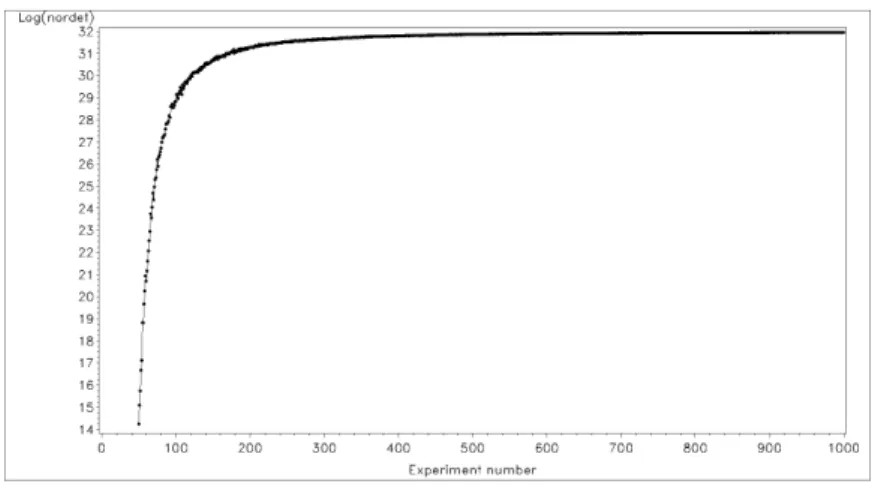
Finally, on the graph of the normalized determinants (or their logarithms) versus n, we can detect a good compromise between a high level of the D-optimality criterion and a reasonable value of n (see Figure 1 in the Application section). Let n be this optimal value of n. The DOCED*, Dn P, is therefore found.
2.3
The novel Sensitivity Indices
These new sensitivity indices, which we refer to under the general term of SIV IP in this article, are based on the V IP statistics obtained in PLSR outputs. The V IP statistics are de…ned by formula (14) given in the Appendix. We propose two types of SIV IP :
the Individual Sensitivity Index de…ned for each k monomial term among the P monomial terms of Md, for univariate and multivariate output, by:
ISIV IPk = V IPk2=P (1)
If the output is multivariate, we refer to it as the Generalized Individual Sensitivity Indexin this case, or GISIV IPk.
the Total d order Sensitivity Index de…ned for each of the p original inputs, for univariate and multivariate output, by:
TdSIV IPj = J
X
u=1
ISIV IP ju (2)
where ju is the uth index set where a j index appears, J is the total
num-ber of these ju, and ISIV IP ju is the corresponding monomial individual sensitivity index. For example, with three inputs, X1, X2, X3, and d = 2,
the Total 2 order Sensitivity Index for X1 is expressed as T2SIV IP (X1)
= ISIV IP (X1)+ ISIV IP (X12)+ ISIV IP (X1X2)+ ISIV IP (X1X3). If
the output is multivariate, we refer to it as the Generalized Total d order Sensitivity Indexin this case, or GTdSIV IPj.
We emphasize here that the GISIV IPk and the GTdSIV IPj are particularly
useful from a practical point of view. Indeed, they can reveal several strong or weak inputs for all the outputs studied simultaneously, which is especially useful when the multivariate output is a spectrum, e.g., infra-red spectrum.
3
Justi…cations of the novel approach proposed
3.1
Justi…cation of the PLSR choice
Firstly, we can observe that the PLSR metamodel deals with partial covariances for constructing its th components, h = 1; :::; H. This aspect is clear if we
exam-ine the developped vectorial structure of a th component given in formula (9) of
the Appendix. Indeed, the term cov (Fh 1; Eh 1;j) is a covariance between the
Fh 1 residual matrix and the Eh 1;j residual vector and is therefore a partial
co-variance by de…nition. Formula (9) thus explains why the multicolinearity among the monomials can be correctly taken into account. Moreover, PLSR leads to the approximation ^F0 =PHh=1thrTh, and we therefore obtain for the Yl univariate
output: var( ^Yl) = var(Yl) H X h=1 rlh2var(th); l = 1; :::; L (3)
which is an empirical orthogonal decomposition of the total variance of ^Yl.
More-over, since Yl Y^l, formula (3) gives an approximation of an empirical orthogonal
decomposition of the Yl output. We can then see with formula (9) that the
de-composition (3) is linked to the partial covariances between the Yl output and the
monomial inputs.
3.2
Justi…cation of the D-optimality choice
If we use Ordinary Least Squares Regression (OLSR) for estimating the P 1 coe¢ cient vector of Md with n real data, the variance of the OLS estimator,
^
OLS, has the following well-known form:
var ^OLS = 2 XTnXn 1
(4) where 2 is a constant, unknown, experimental variance. On the basis of (4), we
can see that in order to minimize the variances and covariances of the ^OLS vector
components, which we always want to do, a D-optimal design, Dn P, is a good
choice because
D
n P = Arg max
n P n
det XTnXn = Arg min
n P n
[det XTnXn 1
] (5)
regardlessof the value of the unknown 2.
In the computer experiment framework, if the metamodel is …xed, then 2 is
based on the "i residuals (see Section 2.1), and formula (4) can then makes sense
as well.
Now, if we want to prove that it is also relevant to use D-optimal designs in the PLSR context strictly de…ned in the framework of OLSR then it might be proven that the determinant of an approximation (no exact formula exists) of the ^
P LS variance will be decreased if Xn was based on a D-optimal design instead of
on just any design. This is an open problem at that time. Only some numerical studies show an advantage of using D-optimal designs in the PLS context.
Lastly, it should be emphasized here that the choice of the D-optimality cri-terion is appropriate only if the postulated model is correct. It is for this reason that we assumed a moderate nonlinearity for the computer model and, therefore, a polynomial approximation with d 3.
3.3
Justi…cation of the VIP-based Sensitivity Indices choice
A …rst justi…cation of the V IP -based Sensitivity Indices, instead of a choice based on ^P LS, for example, can be warranted by the fact that it has been observed for
many years and in many studies that the V IP remains much more stable than ^
P LS when h increases. Moreover, the following two important arguments can be
given in favor of this choice. Deriving the SSI
It is possible to directly derive the SSI in the case of independent inputs in some particular situations. If the computer design is orthogonal, Q2
G = 1, and
L = 1 (one univariate output Yl is considered), then only one PLS component will
be extracted. Its corresponding vectorial form will then be t1 = E01w11+ +
E0Pw1P, and formula (8) becomes F0l = w11+ + w1P because the r vector
becomes the scalar r = 1 and var(E0j) = 1; j = 1; ::: ; P. These w1j2 are equal
to cor2(F
0l; E0j) = cor2(Yl; Zj). In this case, we can prove that w21j is the SSI for
the input Zj. For an input Zj, we have:
ISIV IPj = V IPj2=P = P 1 P cor2(Y l; t1) 1 cor2(Yl; t1) w1j2 = w 2 1j (6)
= cor2(Yl; Zj) = V (E(YljZj))=V (Yl) = SSIj
Summation of the ISIV IPj
As a result of the property given in the Appendix, in the general case (uni-variate or multi(uni-variate outputs), for dependent or independent inputs, we have PP
j=1ISIV IPj = 1, which is a very convenient formula from a practical point
of view if we wish to compare the ISIV IPj to each other. It is analog to the
Sobol’ theoretical summation [7] for independent inputs PQj=1SSIj = 1, where
Q = 2p 1:
Illustration of the SIVIP method for the Ishigami function
In GSA, this function is a very well known test function with three independent inputs [9]. Even if the SIVIP method is speci…cally designed for dependent inputs, it can be relevant to apply it in this situation. Therefore, with a DOCED* of only 32 computer experiments (sampled in a 64-Legendre orthogonal array) and several (not full) M3 polynomial metamodels, we obtained accurate estimations of the
three analytical total sensitivity indices (ATSI). For example, with a polynomial metamodel formed by the 11 monomials X1; X3; X1X2; X1X3; X2X3; X13; X12X2;
X1X22; X23; X2X32 and X33, we obtained the following estimations (in %) \AT SI1 =
44:91 (44:83), \AT SI2 = 35:62 (35:58), and \AT SI3 = 19:47 (19:59); the analytical
values are given in brackets.
However, we do not have any e¢ cient algorithm for …nding these correct mono-mials at this time. Only an exhaustive analysis enabled us to …nd them here. In any case, it is not the aim of the SIVIP method to compute sensitivity indices in the situation of independent inputs.
4
A case study in aeronautics
4.1
Presentation of the problem
This methodology has been applied to aircraft InfraRed Signature (IRS) analysis, within the framework of detection performances of infrared sensor estimation [32]. For an aircraft in a given atmospheric environment, the …rst order e¤ects on the IRS are related to the spectral range, the presentation geometry, the aircraft speed and the engine power setting. Several sources of variability lead to a dispersion of the values likely to be observed: weather, aircraft aspect angles, aircraft type and optical properties. These uncertainties in the input data are propagated through the computer model to the output data. Therefore, the simulated result is an interval of possible IRS that should include the IRS measured at a given moment. Note that a single run with the computer model takes approximately 3 minutes (on a 64 bit Sun Fire workstation with four Intel Xeon processors).
Since many of the input factors of our IRS simulation were uncertain, we used a GSA to identify the most important ones. We considered a daylight air-to-ground full-frontal approach in France by a generic aircraft ‡ying at low altitude (800-1200 ft). The infrared sensor was located on the ground, at a distance of 20 kilometers from the aircraft, in the ‡ight direction. The aircraft was assumed to be spatially unresolved by the sensor.
4.2
De…nition of inputs and outputs
Sixteen uncertain original inputs were analyzed. Eight were related to ‡ight con-ditions and IR optical properties of aircraft surfaces: altitude (ALTI), Mach num-ber (MACH), engine power setting (POWERS), emissivity of air intake (EAI), and to aspect angles of the aircraft: cap (CAP), yaw (YAW), roll (ROLL) and pitch angles (PITCH). Eight were related to atmospheric conditions: visibility (VIS), relative humidity (RH), ground air temperature (TA), atmospheric model (MODEL), aerosol model (IHAZE), cloud presence (CLOUDS), base altitude of the cloud layer (HBASE), and hour to compute solar position (HOUR). The three inputs, MODEL, IHAZE and CLOUDS, were qualitative, with two, three and two levels, respectively. The three aerosol models are the modalities of the IHAZE qualitative input: urban (IHAZE1), maritime (IHAZE2) and rural (IHAZE3). By using the three indicator variables of IHAZE, we had a total of 18 inputs. The modalities of MODEL and CLOUDS were coded as 0/1.
The outputs analyzed were the sensor di¤erential irradiances between the target and the background, and we focused both on: (i) the 3-5 m spectrally integrated target intensity, which corresponds to typical infrared sensor spectral ranges, des-ignated as IRStot hereafter; and (ii) a multispectral intensity, integrated on 14 spectral bands equally spaced in the wave-number domain. The usefulness of mul-tispectral or hyperspectral sensors for remote sensing assignments has been proven [33-35], and some studies [36-38] emphasize their potential for target detection.
We are currently working on the speci…cation of a multispectral sensor for di¤erent missions such as aircraft detection or classi…cation, and being able to perform a sensitivity analysis on a multispectral infrared signature is therefore of the utmost importance.
4.3
Construction of the dependent candidate set
We started by building a type of SFD by sampling 20,000 candidate experiments using the estimated distribution of variables related to atmospheric conditions, except for HOUR, and a Sobol low discrepancy sequence for the nine other vari-ables: ALTI, MACH, POWERS, EAI, CAP, YAW, ROLL, PITCH and HOUR, as explained in [3,8].
RH, TA and HBASE were correlated, and their distribution was estimated on the basis of 3200 measured data using a non-parametric kernel reconstruction of marginal distributions, coupled with a dependence modeling based on a Normal copula [39,40]. This modeling was performed using the scienti…c library Open-TURNS (http://www.openturns.org/).
We also obtained a non-parametric reconstruction for the distribution of VIS and CLOUDS. A discrete uniform distribution was associated with the qualita-tive MODEL. The three aerosol models, IHAZE1, IHAZE2 and IHAZE3, are not equally probable in France, and we considered a {0.45; 0.1; 0.45} probability law. At this stage, the SFD* was obtained. With these 18 inputs, we built the design model matrix, X, from this SFD*, by postulating an incomplete Md of
158 monomials: the 13 original continuous inputs, their 13 squared terms, their 13 cubic terms, and the 114 two-input and three-input interaction terms speci…ed by the infrared signature expert. Therefore, the dimensions of X were 20,000 rows and 158 (= P ) columns.
4.4
Construction of the DOCED*
Firstly, since the information matrices, XT
nXn, built with Xn selected in the
pre-ceding X, were generally not invertible, this X matrix was replaced by the Z ma-trix formed by the …rst 50 principal components of a principal component analysis (these 50 components represented 99% of inertia). A DOCED sequence was ex-tracted from the SFD*, from n = n0 = 50 to n = 1000. A good compromise was
obtained in 180 experiments between the maximization of the (log) normalized determinant (see Step 2 in Section 2.2) and the number of runs, if we observe Figure 1. The DOCED*, Dn =180;P =158, was then formed with n = 180.
4.5
Results and discussion
We focused here on the total indices, the T3SIV IP and the GT3SIV IP, since it
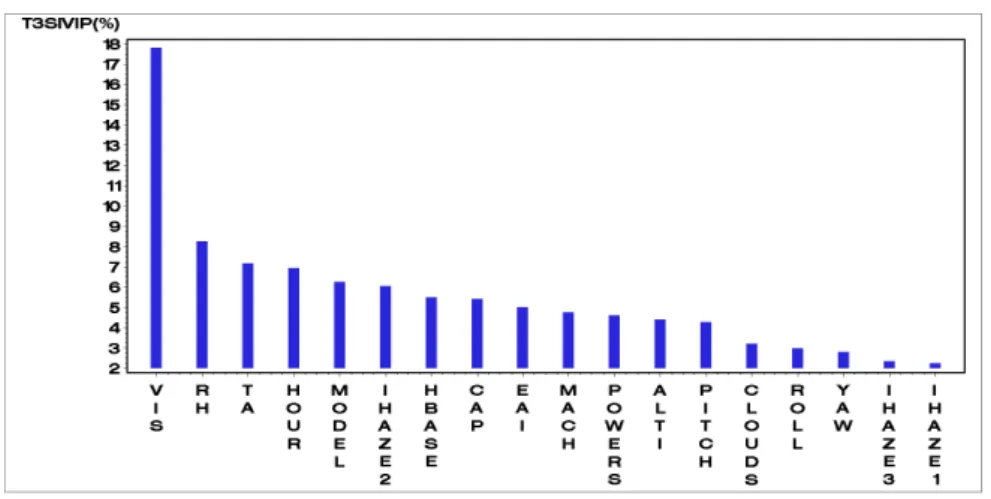
was quite di¢ cult to analyze all of the 158 monomial ISIVIP. However, it should be noted that the 20 largest ISIVIP and GISIVIP were associated with terms involving VIS or IHAZE2, and that the largest one-degree monomials were also associated with VIS and IHAZE2. The bar plot of Figure 2 presents the T3SIV IP
(in %) associated with the 18 variables.
The total IHAZE input contribution can be computed by summing the T3SIV IP
corresponding to the IHAZE1, IHAZE2 and IHAZE3 indicator variables. The T3SIV IP associated with IHAZE is then 10.65, corresponding to the second
high-est T3SIV IP in comparison with the others. Thus, two variables are particularly
predominant: VIS and IHAZE and, more precisely, the maritime model of aerosol 10
Figure 1: Evolution of the normalized determinant logarithm versus the number of experimentsn.
IHAZE2, since indices associated with the two other models, IHAZE1 and IHAZE3 (urban and rural), are the lowest ones. This can be explained by the fact that ur-ban and rural aerosols are quite similar and very di¤erent from the maritime one. Three additional variables also have an important impact on IRS variability: RH, TA and HOUR. It is then di¢ cult to discriminate among the following eight vari-ables in terms of total indices: MODEL, CAP, HBASE, EAI, MACH, POWERS, ALTI and PITCH. CLOUDS, ROLL and YAW have relatively negligible contri-butions to IRS variability since their total indices represent less than 10% of sum of all of the indices.
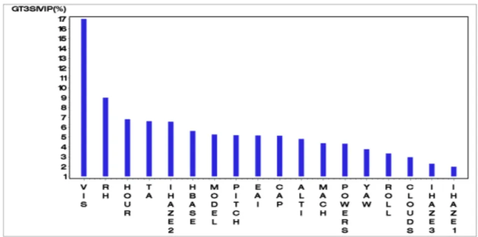
If we now focus on the multispectral infrared signature, the bar plot of Figure 3 presents the GT3SIV IP (in %) associated with the 18 variables. As previously
mentioned, the GT3SIV IP associated with the total IHAZE contribution is
com-puted by summing the GT3SIV IP corresponding to the IHAZE1, IHAZE2 and
IHAZE3 indicator variables. Their sum is 10.8 and corresponds to the second highest GT3SIV IP in comparison with the others. Hence, as in the IRStot case,
the two predominant variables are VIS and IHAZE. The three additional variables that also have an important impact on IRS variability are unchanged: RH, TA and HOUR. The main di¤erence with IRStot stems from the higher indices corre-sponding to the three angles: PITCH, which extends from rank 13 up to rank 8, and, to a lesser extent, YAW and ROLL, which remain without in‡uence. A possi-ble explanation is that some of the 14 bands signi…cantly emphasize the impact of phenomena that vary with aspect angles, such as the plume emission contribution or the airframe re‡ected light from the surrounding background.
Figure 2: The 18 T3SIV IP (in %) corresponding to the 18 inputs for the IRStot
univariate output.
Finally, only …ve variables among the whole set actually in‡uence the spectrally integrated and the multispectral infrared signature variability for the scenario con-sidered, and they are all atmosphere-related factors. If we want to reduce the IRS uncertainty, we can thus combine the optics sensor with some detectors that can measure these atmospheric data. By virtue of the scenario chosen, a full frontal approach, large variations in IRS due to changes in aircraft aspect angle are ex-cluded. The variations in aspect may dominate the rest of the variables. Hence, by essentially …xing the aspect to focus on, the variability of the meteorological phenomena may be given more importance in the overall IRS than if viewed from a di¤erent angle. Secondly, the low aircraft altitude and the long path between the sensor and the aircraft lead to an optical path that crosses the lowest atmospheric layers.
Consequently, the infrared transmission between sensor and aircraft and the atmospheric radiance, which both have a strong impact on the sensor di¤erential irradiance, are themselves in‡uenced by the quantity and type of low altitude atmospheric aerosols. Even if the sensitivity analyses of the multispectral and the spectrally integrated IRS lead to rather similar results for our scenario, it is especially interesting to be able to perform a sensitivity analysis in dozens of spectral bands simultaneously. We can thereby consider di¤erent selections and mergings of bands in order to perform the speci…cation of a multispectral sensor.
Figure 3: The 18GT3SIV IP (in %) corresponding to the 18 inputs for the multivariate
output.
5
Conclusions
5.1
Application aspects
Thanks to the methodology proposed in this paper, we were able to identify …ve variables that have a strong impact on integrated and multispectral IRS variability for the chosen scenario with only 180 simulations, and we can now proceed to the next step, the establishment of an IRS simulation metamodel, in order to be able to estimate IRS dispersion. Since these …rst results are quite promising, it would be interesting to extend this model to other scenarios with more uncertain variables, and to other military objects.
5.2
Methodological aspects
Our method, designated the SIVIP method, is based on two very well-established theories (PLS regression and D-optimal designs), and it is very simple and very easy to put into practice by means of an SAS/IML procedure or an R-language procedure, both available upon request to the corresponding author (the SIVIP R-package will soon be available on the CRAN). To our knowledge, no other practical method exists to simultaneously manage the A, B and C constraints, notably with multivariate outputs and, therefore, no realistic comparison of our method can be made today with an alternative method. Only scienti…c experts in the …eld are quali…ed to validate the results at this time. This has been done in the real application problem presented in Section 4, as well as in the application presented in [15] with success. We hope that new competitive methods will be developed
in the near future, which will then make it possible for the researchers involved to test our dataset using their own methods. It should also be noted that even with independent inputs, this method can be useful in the frequently encountered situation of costly simulations, even if the SIVIP will generally be di¤erent from the SSI (even in this particular situation of independent inputs).
The SIVIP method works correctly in the situation where the user can postulate that the nonlinearity of the computer model is reasonable, i.e., if d 3. Many real applications fall within this framework. However, if no prior knowledge is available about the nonlinearity, then neither the value of d nor the structure of the polynomial metamodel can be assumed (no previously chosen monomials are possible). In this situation, giving a large value to d can be a dangerous choice because of the well-known poor behavior of high-degree polynomials in terms of approximations. To address this di¢ culty, we propose an adaptive - and therefore parsimonious, in terms of the total simulation run number - version of the method for strong nonlinear computer models, which is currently being developed.
Acknowledgments: We would like to thank Gail Wagman, a professional English language translator, who corrected the English, and Régis Lebrun, from EADS Innova-tion Works, who performed the dependence modeling based on copulas.
References
[1] A. Saltelli, Sensitivity Analysis for Importance Assessment, Risk Analysis 22 (2002), pp. 579-590.
[2] M. Ellouze, J.P. Gauchi, and J.C. Augustin, Sensitivity analyses applied to an exposure model of Listeria monocytogenes in smoked cold salmon, Risk Analysis 30(5) (2010), pp. 841-852.
[3] A. Saltelli, K. Chan, and E.M Scott (Editors), Sensitivity analysis, Wiley, New York, 2000.
[4] A. Saltelli, S. Tarantola, F. Campolongo, and M. Ratto, Sensitivity analysis in practice - A guide to assessing scienti…c models, Wiley, New York, 2004.
[5] I.M. Sobol’, Sensitivity estimates for nonlinear mathematical models, Mathe-matical Modeling Computational Experiments 1 (1993), pp. 407-414.
[6] A. Saltelli, Making best use of model evaluations to compute sensitivity indices, Computational Physics Communications 145 (2002), pp. 280-297.
[7] I.M. Sobol’, Global sensitivity indices for nonlinear mathematical models and their Monte Carlo estimates, Mathematics and Computers in Simulation 55 (1-3) (2001), pp. 271-280.
[8] K.T. Fang, R. Li, and A. Sudjianto, Design and modelling for computer exper-iments, Chapman and Hall / CRC, London, 2006.
[9] B. Sudret, Global sensitivity analysis using polynomial chaos expansions, Reli-ability Engineering & System Safety 93 (2008), pp. 964-979.
[10] G. Blatman and B. Sudret, Adaptive sparse polynomial chaos expansion based on Least Angle Regression, Journal of Computational Physics 230 (6) (2011), pp. 2345-2367.
[11] J. Jacques, C. Lavergne, N. Devictor, Sensitivity analysis in presence of model uncertainty and correlated inputs, Reliability Engineering & System Safety 91 (2006), pp. 1126-1134.
[12] H. Rabitz, Global Sensitivity Analysis for Systems with Independent and/or Correlated Inputs, Procedia Social and Behavioral Sciences 2 (2010), pp. 7587-7589.
[13] T.A. Mara and S. Tarantola, Variance-based sensitivity indices for models with dependent inputs, Reliability Engineering & System Safety 107 (2012), pp. 115-121.
[14] S. Kucherenko, S. Tarantola, and P. Annoni, Estimation of global sensitivity indices for models with dependent variables, Computer Physics Communications 183 (2012), pp. 937-946.
[15] J.P. Gauchi, S. Lehuta, and S. Mahévas, Optimal Sensitivity Analysis under Constraints: Application to Fisheries, Procedia Social and Behavioral Sciences 2 (2010), pp. 7658-7659.
[16] J.P. Gauchi and S. Lefebvre, PLS-based global sensitivity analysis for numerical models: an application to aircraft infrared signatures, In: Proceedings of PLS2012, the 7th International Conference on PLS and Related Methods, (2012), pp. 43–45, Houston, Texas, USA.
[17] S. Lefebvre and J.P. Gauchi, Multidimensional Global Sensitivity Analysis for Aircraft Infrared Signature Models with Dependent Inputs, 7th International Conference on Sensitivity Analysis of Model Output, July 1-4 2013, Nice, France. [18] J. Sacks, S.B. Schiller, and W.J. Welch, Design for computer experiments, Technometrics 31(1) (1989), pp. 41-47.
[19] T.J. Santner, B.J. Williams, and W.I. Notz, The Design and Analysis of Computer Experiments, Springer, New York, 2003.
[20] P.Z.J. Qian, H. Wu, and C.F.J. Wu, Gaussian process models for computer experiments with qualitative and quantitative factors, Technometrics 50(3) (2008), pp. 383-396.
[21] M. Lamboni, H. Monod, and D. Makowski, Multivariate sensitivity analy-sis to measure global contribution of input factors in dynamic models, Reliability Engineering & System Safety 96(4) (2011), pp. 450–459.
[22] A. Marrel, B. Iooss, M. Jullien, B. Laurent, and E. Volkova, Global sensitivity analysis for models with spatially dependent outputs, Environmetrics 22(3) (2011), pp. 383–397.
[23] A.C. Atkinson and A.N. Donev, Optimum experimental designs, Clarendon Press, Oxford, UK, 1992.
[24] V.V. Fedorov, Theory of optimal experiments, Academic Press, New York, 1972.
[25] M.D. McKay, R.J. Beckman, and W.J. Conover, A comparison of three meth-ods for selecting values of input variables in the analysis of output from a computer code, Technometrics 21 (1979), pp. 239-245.
[26] R.L. Iman, W.J. Conover, A distribution-free approach to inducing rank corre-lation among input variables, Communications in Statistics-Simucorre-lation and Com-putation 11 (1982), pp. 311-334.
[27] R.B. Nelsen, An Introduction to Copula 2nd Ed., Springer, New York, 2006. [28] H. Joe, Multivariate Models and Dependance Concepts, Chapman & Hall, New York, 1997.
[29] J.P.C. Kleijnen, W. van Beers, and I. van Nieuwenhuyse, Constrained opti-mization in expensive simulation: Novel approach, European Journal of Opera-tional Research 202 (2010), pp. 164-174.
[30] T.J. Mitchell, An algorithm for the construction of D-optimum experimental designs, Technometrics 16 (1974), pp. 203-210.
[31] SAS Software, QC module, Optex procedure, Version 9.2, SAS Institute, North Carolina, USA, 2011.
[32] S. Lefebvre, A. Roblin, S. Varet, and G. Durand, A methodological approach for statistical evaluation of aircraft infrared signature, Reliability Engineering & System Safety 95 (2010), pp. 484-493.
[33] L.E Ho¤, A.M. Chen, X. Yu, and E.M. Winter, Enhanced Classi…cation Per-formance from Multiband Infrared Imagery, In: Proceedings of the 30th IEEE Asilomar Conference on Signals, Systems and ComputersAsilomar, 29 (1996), pp. 837-841.
[34] C.I. Chang, S.S. Chiang, Anomaly detection and Classi…cation for Hyperspec-tral Imagery, IEEE Trans. Geosci. Remote Sensing 40 (2002), pp. 1314-1325. [35] U. Amato, A. Antoniadis, V. Cuomo, L. Cutillo, M. Franzese, L. Murino, and C. Serio, Statistical cloud detection from SEVIRI multispectral images, Remote Sensing of Environment 112 (2008), pp. 750-766.
[36] J. Karlholm and I. Renhorn, Wavelength band selection method for multispec-tral target detection, Applied Optics 41 (32) (2002), pp. 6786-6795.
[37] J. Ahlberg and I. Renhorn, Multi and Hyperspectral Target and Anomaly De-tection, Scienti…c Report of the Swedish Defence Research Agency (FOI), FOI-R-1526-SE, 2004.
[38] D. Manolakis, G. Shaw, Detection algorithms for hyperspectral imaging appli-cations, IEEE Signal Process. Mag. 19 (2002), pp. 29-43.
[39] R.B. Nelsen, An Introduction to Copula 2nd Ed., Springer, New York, 2006. [40] H. Joe, Multivariate Models and Dependance Concepts, Chapman & Hall, New York, 1997.
[41] H. Martens and T. Naes, Multivariate calibration, Wiley, New York, 1992. [42] M. Tenenhaus, J.-P. Gauchi, and C. Ménardo, Régression PLS et Applications. Revue de Statistique Appliquée XLIII(1) (1995), pp. 7-63.
[43] M. Tenenhaus, Régression PLS - théorie et pratique, Technip, Paris, 1998. [44] S. Wold, M. Sjöstrom, and L. Friksson, PLS Regression: a basic tool of chemo-metrics, Chemometrics and Intelligent Laboratory Systems 58 (2001), pp. 109-130. [45] N. Kettaneh-Wold, Analysis of mixture data with partial least squares, Chem Intel Lab Sys 14 (1992), pp. 57-69.
[46] H. Wold, Estimation of principal components and related models by iterative least squares, in Multivariate Analysis, Krishnaiah PR (Ed.). New York, Academic Press (1966), pp. 391-420.
[47] SIMCA-P9 software, User Guide and Tutorial, Umetrics AB, Umea, Sweden, 2001.
[48] A. Lazraq, R. Cléroux, and J.-P. Gauchi, Selecting both latent and explanatory variables in the PLS1 regression model, Chemometrics and Intelligent Laboratory Systems 66 (2003), pp. 117-126.
Appendix: PLSR background A brief overview of PLSR
PLSR is a bilinear method for relating inputs to outputs, and that is very popular in the chemometrics …eld [41-44]. It is very di¤erent (particularly from the algorithm point of view) from the familiar Ordinary Least Squares Regression (OLSR) in that no matrix inversion is needed. For the sake of clarity, we use input notations in this Appendix that are di¤erent from those used in the other sections of this paper. Bold characters are used for vectors and matrices, but standard characters are used when a general meaning is assumed, e.g., a PLS component is designated asth, whereas in its vectorial form, it
is designated asth.
The general goal of PLSR is to model, via linear combinations, the link between R
explanatory (input) variables j, j = 1; : : : ; R, and L (> 1) responses (outputs) Yl,
l = 1; : : : ; L, both observed on the sameN objects. We can represent the PLSR model by using the multivariate model form:
YN L= N R R L+ N L (7)
whereYN Lis the observed multivariate ouput matrix, N Ris the input matrix, R L
is a (R L)-matrix of coe¢ cients to be estimated, and N Lis a (N L)-matrix of error
terms. PLSR presents some very strong advantages over OLSR: (i) the input variables - monomials built with these input variables can also be taken into account, including quadratic terms, interactions terms, cubic terms, etc. - can be highly correlated or even functionally linked, whereas the ^P LS estimates of R L remain interpretable (e.g., see
the very well illustrated example in [45] where the inputs add up to one at each row of the design matrix); (ii) R and/or L can be larger than N; (iii) information about the probability distributions of the elements is not needed (it is considered to be a so-called distribution-free method). The …rst two cases, (i) and (ii), make it impossible to use OLSR. The PLSR algorithm is based on a very speci…c algorithm, the NIPALS algorithm [43,46,47]. Following are some formal elements.
Let E0 be the centred and scaled matrix (i.e., mean = 0 and variance = 1 for
each column);F0, the centered and scaledY matrix; Eh, the residual matrix from the
decomposition of E0 by usingh PLS components, th; Fh, the residual matrix from the
decomposition ofF0by usinghPLS components;Flh, thelthcolumn ofFh; andH, the
PLS component number retained. Therefore, the PLSR objective is to construct a linear combination, u1 = F0c1, with columns of F0, and a linear combination, t1 = E0w1,
with columns of E0, by the maximization of the covariance between the t1 and u1
components, subject to the constraints kw1k2 = kc1k2 = 1. Hence, we obtain two
variables, u1 and t1, as correlated as possible, and best summing up E0 and F0: The
following regressions:
E0 = t1pT1 + E1
F0 = t1rT1 + F1
are then performed. The E0 and F0 are de‡ated by t1pT1 and t1rT1, and second linear
combinations,u2 and t2, are computed, and so on. We …nally obtain:
F0 = t1rT1 + : : : + thrTh + Fh (8)
where thethare orthogonal between them. We can develop the vectorial form of thas:
th= " P X j=1 cov2(Fh 1; Eh 1;j) # 1=2 P X j=1 [cov (Fh 1; Eh 1;j)] Eh 1;j (9)
On the basis of (8), we can deduce the following norm decomposition, i.e., an em-pirical decomposition of the output variance (because the Fl0 in F0 are centered and
scaled):
kF0k2 =kr1k2kt1k2+ : : : +krHk2ktHk2+kFHk2 (10)
For one (univariate) centered-scaled output,Fl0, we can then write:
kFl0k2 = var(Fl0) = r21kt1k2+ : : : + r2HktHk2+kFlHk2 (11)
The signi…cant number H of PLS components is given by means of a speci…c cross-validation test (see the end of this Appendix).
On the basis of (8) we can obtain the PLS regression equations:
^
Yl = ^l0+ ^l1 1+ : : : + ^lM M ; l = 1; :::; L
De…nition of the V IP statistics in PLSR
Let the redundancy statistics be as follows:
Rd(Y ; th) = 1 L L X l=1 cor2(Yl; th) , L 1 (12) and Rd(Y ; t1; : : : ; tH) = H X h=1 1 L L X l=1 cor2(Yl; th) , L 1 (13)
The V IP (Variable Importance in the Projection) statistics [43,47] for an j input in
the presence of a univariate or multivariate Y output is then de…ned as:
V IPHj = " P Rd(Y ; t1; : : : ; tH) H X h=1 Rd(Y ; th)whj2 #1=2 (14)
where the whj are the components of the wh vectors. Note the important property
PP
j=1V IPHj2 = P.
Obviously, the V IP statistics make sense if the value of the …tting-prediction cri-terion, Q2
G, (see below) is close enough to one, implying that M =^ N R^R L is a
reasonable estimated approximation of the unknown underlying model for both …tting and prediction. In Section 2.3, we omitted the index H for the sake of brevity be-cause non-ambiguity is possible once M^ has been cross-validated with H components by means of the Q2
G:
Validation of the PLSR model
The PLSR model is validated by a cross-validation procedure based on the Q2 Gh and
Q2
G statistics (bounded between 0 and 1) computed for each univariate output, detailed
in [48]. The PLSR model is thus iteratively built, and these iterations are stopped by means of a procedure on the th components. A commonly used procedure is the one
inspired by the rule proposed in [47]. This rule is the following: a th component (from
h = 1) is retained if Q2Gh 1 (0:95)2. Finally, with the H retained components, the
Q2
G cumulated index is computed [47]. Thus, thisQ2G index is a …tting-prediction type
criterion typically designed for a PLSR model. Its major advantage, in comparison to a classical R2, is that it avoids over…tting. From a practical point of view, we have to choose aQ2
G threshold to be overtaken of at least 0.80.