Magneto-acoustic resonance in a non-uniform current carrying plasma column

Printed in Great Britain

Magneto-acoustic resonance in

a non-uniform current carrying plasma column

By J. VACLAVIK

Department of Physics, University of Fribourg (Received 17 March 1971)

The forced radial magneto-acoustic oscillations in a plasma column with non-uniform mass density and temperature are investigated. It turns out that the oscillations have a resonant character similar to that of the magneto-acoustic oscillations in a uniform plasma column. The properties of the axial and azi-muthal components of the oscillating magnetic field are discussed in detail.

1. Introduction

An investigation of magneto-acoustic resonance is of considerable interest in problems connected with the development of methods of the high frequency heating of plasma. It was shown theoretically by Frank-Kamenetskii (1960a, b) that the forced radial oscillations of a uniform plasma column immersed in a uni-form axial magnetic field have a resonant character when the forcing frequency approaches one of the natural frequencies of the plasma column. This pheno-menon, which is called magneto-acoustic resonance, has actually been observed and investigated (by e.g. Kovan et al. 1962; Cantieni & Schneider 1963; Borodin et al. 1963; Faessler, Vaclavik & Schneider 1969). All the investigations have been made for a plasma where the mass density is uniform throughout.

In this paper, the properties of magneto-acoustic resonance in a plasma column possessing non-uniform density and temperature distributions are treated. The column is immersed in a uniform axial magnetic field and carries a uniform axial current. On the surrounding walls an azimuthal oscillating current is excited.

2. Basic equations

We now proceed to write the basic equations needed to describe the character of the oscillations inside the column. Let po,po, Bo, j0 represent the equilibrium

values of the mass density, pressure, magnetic field and current density. The linearized equations of magneto-hydrodynanics can then be written in the form,

Owr 1

B]), (1)

: 0, (2) (3)

(4) (5) where E is the electric field, v the plasma velocity, y the adiabaticity index and

o the conductivity tensor.

In what follows we adopt a cylindrical co-ordinate system r, <j>, z, and assume that djd<j> = djdz = 0 throughout. For the equilibrium quantities of the plasma, we can then use the simplified model of pinched plasma column. Thus

(6)

Jo ~ lz3o>

where B is the radius of the column, and i^ and i3 are the unit vectors in the

azi-muthal and axial directions, respectively.

Finally, (l)-(5) must be completed by a boundary condition. Consistently with our assumptions, we may write it as

B = isBexcos<ot where w is the forcing frequency.

3. Uniform temperature case

Equations (l)-(5) are too hard to solve in general. Therefore, we only con-sider some special cases. We study first the case when the equilibrium plasma temperature is uniform over the column cross-section. From (6) it then follows that

( ( ) ) (8) p* being the mass density at the centre of the column, cA = Baj{4mp*)^ the Alfve"n velocity and S = B0<p(R)IB0.

Let us, for a while, assume that o -+ oo. Thus, setting j = 0 in (3), introducing the time dependence exp ( - iwt) and eliminating the quantities j and j0 by means

of (4) and (6), respectively, we obtain the following equations:

dp0 Id

(9)

^ - T 9 . (ID C &2 = -z-^5Bv (1 2) C l " - > (13) £ . = - - — < (14) where v = vr.

Although the quantities of interest are the magnetic field components Bz and

B$, from the mathematical point of view it is more convenient to solve the equa-tions governing the electric field components E^ and Es. On making use of (8), (9)-(14) can be reduced to one equation involving the quantity E^. This is accom-plished by eliminating^), v, Ez, Bs, B^ by (10)-( 14), respectively. Now, (9) becomes

E_*' ( 1 5 )

where r = rjR and w = o)R\cA.

Since the solution of (15) for arbitrary values of d is difficult, we confine our-selves to the limiting case S2 <| 1. The electric field component Eu, with the accur-acy up to the first order of the parameter 8, is then given by the solution of the equation, , ,

(16) With the same accuracy, the electric field component Ez is obtained by combining (11) and (12) as E.—irE,, (17)

EQ being the solution of (16).

We now return to the case when the conductivity is finite and assume that WC2_/(4TTCT

XC^) <^ 1. Hence, by means of (3)-(5), it can easily be shown that (16)

is to be replaced by

^ = 0, (18) where a = c2l(i7Tcr±RcA) <^ 1. As far as the quantity Ez is concerned, it is suffi-cient to use the approximate formula (17).

Equation (18) can be reduced to simpler form by making the transformation, x = wr2, E^x) = xle-l*i/r{x). (19) This transformation reduces (18) to

where a = 1 — \u).

t/r = ^rC) + aipM +..., and confine ourselves to the first two terms of the expansion. It is evident that the functions ^0 ) and ifi®1 satisfy

d^<)_ = -i«(5J_a;)»ijr<«. (22)

dx r v

dx2 dx

Equations (21) and (22) are homogeneous and inhomogeneous confluent hyper-geometric differential equations, respectively. The only solution of (21), which is

regular at x - 0, is #» - AM(a,2,x), (23)

A being an arbitrary constant. M(a, 2, x) is the Kummer's function (Abramowitz & Stegun 1965), defined by the series

where Y is the gamma function.

The solution of (22) can be found by variation of constants. The fundamental system of solutions of the considered differential equation is represented by the functions M(a,2,x) and U(a, 2,x) (Abramowitz & Stegun), the latter being defined by the relation,

|T'(a + n) P(2 + n) 1 ]\

1 ]\

l + n\j

]

T(2 + n) l + n\j xT(ay

W{M, U} of the functions M and V is given by

"vw—ma-

( 2 4

»

On taking into account (23) and (24), the solution of (22) is obtained in the form, r» = liAT(a){U(a,2,x)I(M,x)-M(a,2,x)I(U,x)}, (25)

I(M,x)= fXMZ(a,2,y)e-v(y-G>)*ydy,

Jo

I(V,x) = \X M{a,2,y)V{a,2,y)e-v{y-(oYydy. Jo

The complete solution of (20), with the considered accuracy, is given by the per-tinent superposition of the solutions ^0 ) and ^<1). Reapplying the transformation (19), and using (13) and the boundary condition (7), we determine the constant A. The final solution for the electric field component E^ is then found as

, (26a) c

M{a.,2,aJf2){l-liar(a)I(U,a}r2) + Jtor(a) C/(a, 2,wr2)/(if, w2)

D{x) = (2-x) F(x) =

(2-(266)

( 26c) The magnetic field component Be is easily obtained from (26) by means of (13). Thus,

D((Dr2) {1 - iiaT(a) I( U, Tor2)} + iiaTja) F(wr*) I(M, air2) Finally, combining (13), (14) and (17) we find

£,(r) = 8fB.(r).

( '

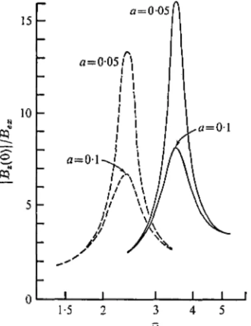
(28) It is obvious that the amplitudes of the magnetic field components Bz and B$ are given by \BS\ and \B^\, respectively. Figure 1 shows the variation of the Bz amplitude with the frequency w, at the centre of the plasma column. The dashed lines represent the Bz amplitude in the case when the mass density is uniform over the column cross section and equals p* (Cantieni & Schneider). We see that, in the non-uniform column, the magneto-acoustic resonance occurs at the frequency To x 3-5 which is higher than the resonant frequency in the case of the uniform column (w x 2-4). Moreover, we note that in the resonance, the magnetic field amplitudes are higher as compared with those corresponding to the uniform plasma. Figures 2 and 3 show the variation of the Be and B^ amplitudes with the radius f, in the resonance. Here again the dashed lines correspond to the case of the uniform plasma. It is seen that the magnetic field component Bs is confined

15 10

o

FIGURE 1. Variation of the axial component of magnetic field with frequency. 3 4 5

largely to the central region of the column, decaying quite rapidly towards the edges. On the other hand, the B^ component is confined largely to the neighbour-hood of the point r — 0-4.

15 10

SL

FIGUBE 2. Variation of the axial component of magnetic field with radius. 5=3-5

K|

a=005

0-2 0-4 0-6 0-8 10

FIGUBE 3. Variation of the azimuthal component of magnetic field with radius.

4. Non-uniform temperature case

In § 4 we consider the effects of a non-uniform temperature. For simplicity, we set 8 = 0 and assume the equilibrium plasma temperature to possess the following radial distribution: T = T*(l — ef2) (0 < e < 1), (29) T* being the temperature at the centre of the column. According to Spitzer's (1956) formula for the conductivity, we can then write the approximate relation

It is easily seen that (18) is now replaced by

= 0, (31)

where a* = c2l(<±narlRcA).

On re-applying the procedure used in § 3 to (31), we find the following expression for the magnetic field:

*)} + jia* T(a) F(wr2) K(M, W*) D(<Dr2) {1 - lia*T(a) K{ U,

Jo

(326)

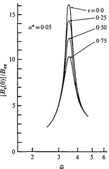
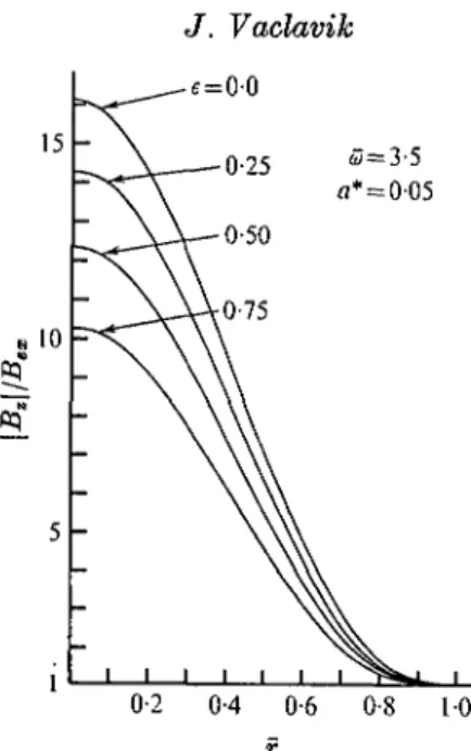
(32c) Figures 4 and 5 show the variation of the magnetic field amplitude with the frequency To and with the radius r, respectively, for some typical values of the parameter e. We note that the greater the temperature inhomogeneity, the smaller is the resonant amplitude of the magnetic field. Furthermore, we see that the effects of the non-uniform temperature are largely manifested in the central region of the column.

15

10

a?

a* = 005

FIGURE 4. Variation of magnetic field with frequency in the case of non-uniform temperature.

£ = 00

o* = 005

0-2 0-4 0-6 0-8 10

FIGURE 5. Variation of magnetic field with radius in the case of non-uniform temperature.

The author is grateful to Prof. 0 . Huber and Prof. H. Schneider for their con-tinued interest in this work. The work was supported by the Swiss National Science Foundation.

R E F E R E N C E S

ABBAMOWITZ, M. & STEGUN, I. A. 1965 Handbook of Mathematical Functions. Dover.

BORODIN, A. V., KOVAN, I. A., RAKHIMBABAYEV, Y. R., RUSSANOV, V. D., SMIBNOV, V. P., FBANK-KAMENETSKII, D. A. 1963 Nuc. Fus. 3, 38

CANTIENI, E. & SCHNEIDEB, H. 1963 Helv. Phys. Acta, 36, 993.

FAESSLEB, K., VACLAVIK, J. & SCHNEIDER, H. 1969 Helv. Phys. Acta, 42, 23.

FBANK-KAMENETSKII, D. A. 1960a Zh. exp. te.or.fiz. 39, 669. FRANK-KAMENETSKII, D. A. 19606 Zh. tekh.fiz. 30, 899.

KOVAN, I. A., PATBUSHEV, B. I., RUSSANOV, V. D., TILININ, G. N., FBANK-KAMENETSKII,

D. A. 1962 Zh. exp. teor. fiz. 43, 16.