Studies in Nonlinear Dynamics &
Econometrics
Volume , Issue Article
A Nonlinear Analysis of Forward
Premium and Volatility
Chiente Hsu
Peter Kugler
University of Bern
University of Bern
ISSN: 1558-3708
Studies in Nonlinear Dynamics & Econometrics is produced by The Berkeley Electronic Press (bepress). All rights reserved.
A Nonlinear Analysis of Forward Premium and Volatility
Chiente Hsu1 Peter Kugler Department of Economics University of Bern hsuct@econ.duke.edu kugler@vwi.unibe.chAbstract. In this paper we investigate the relationship between risk premium and a time-varying conditional variance of spot rate using weekly Swiss franc/US dollar exchange-rate data. First, we apply an
EGARCH-in-mean framework to test the unbiasedness hypothesis of the forward rate with a volatility dependent risk premium. The corresponding estimates point to no significant influence of volatility on the risk premium, and reject the unbiasedness hypothesis. Second, we apply a seminonparametric, nonlinear impulse-response analysis to the spot-rate change and the forward premium. This framework allows us to analyze the risk premium/volatility relationship without using a specific, parametric model such as EGARCH-in-mean. The latter analysis confirms the negative EGARCH-in-mean results with respect to the risk premium/volatility relationship, although the volatility dynamics estimated is clearly different from that implied by the EGARCH estimate. Moreover, the forward premium has a nonlinear dynamic influence on the spot rate, whereas the converse is not true.
Keywords. Forward and spot exchange rates, Unbiasedness hypothesis of the forward rate, ARCH-in-mean, Seminonparametric procedure, Nonlinear impulse response
1 Introduction
A widely recognized anomaly in the foreign exchange market is the rejection of the unbiasedness hypothesis for the forward rates as predictors of the spot rates. This anomaly has spawned numerous papers attempting to account for it. One of the most influential explanations of the negative results has been to attribute the empirical failure to a time-varying risk premium (Fama1984). The ARCH-in-mean model introduced by Engle, Lilien, and Robbins (1987) is perhaps the most popular model attempting to tie the risk premium to a
time-varying conditional variance. However, the success relating the risk premium to the conditional variance is rather mixed. On the one hand, using weekly data for the Australian/US dollar, Kendall and McDonald (1989) find significant estimate for a GARCH(1, 1)-in-mean model. On the other hand, Domowitz and Hakkio (1985) find little evidence of ARCH-M effects for monthly returns from holding five foreign currencies. Bekaert and Hodrick (1993) use ARCH as well as GARCH models, and find that considerable variation in the risk premium remains even if one takes the conditional variance of the spot rate into account.
1Helpful comments from an anonymous referee and from the editor are gratefully acknowledged. We are especially grateful to George Tauchen,
As pointed out by Pagan and Ullah (1988), consistent estimation in the ARCH-in-mean model requires the full model to be correctly specified. Any misspecification in the variance equation generally leads to a biased and inconsistent estimate of the parameters in the mean equation. Further evidence of the sensitivity of the parameter estimate in the ARCH-in-mean model with respect to different model specifications is given in Bollerslev, Chou, and Kroner (1992). Therefore, the controversial evidence for a conditional mean-variance relationship in the foreign exchange market may be caused by misspecifications of the models used.
In this paper, we reconsider the relationship between the risk premium and a time-varying volatility using a weekly data set for the Swiss franc/US dollar exchange rate covering the period 1977 to 1991. First, we test the unbiasedness hypothesis of the forward rate, taking into account a risk premium depending on the volatility of the spot rate in an EGARCH-in-mean framework. This exercise leads to a clear rejection of the unbiasedness hypothesis and shows an insignificant effect of the conditional variance on the risk premium. Second, we ask whether this negative result can be attributed to misspecifications of the mean and variance equations. To this end, we undertake a nonlinear impulse-response analysis by utilizing the method
developed by Gallant, Rossi, and Tauchen (1993). This seminonparametric estimation strategy allows us to compare the responses of the reactions of conditional mean and variance of the spot-rate change and the forward premium to shocks without relying on specific parameterizations of mean and variance equations. The results of the EGARCH model are confirmed qualitatively by this exercise.
The remaining part of the paper is organized as follows. Section 2 contains empirical results for the standard test of the unbiasedness hypothesis of the forward rate, as well as results on the conditional mean-volatility relationship of Swiss franc/US dollar exchange rates using the EGARCH-in-mean model. Section 3 provides a brief introduction to the nonlinear impulse-response analysis and presents the empirical results obtained with our data. Section 4 concludes the paper.
2 The Unbiasedness of the Forward Exchange Rates and ARCH-In-Mean Model: A Preliminary Exploration
Under risk neutrality, forward rates are market predictions of future spot rates. Hence, the basic equation to test the unbiasedness of the forward rate is
st+1 = α + βft + et+1, (1)
where st denotes the spot rate, ft denotes the forward rate, and the serially uncorrelated mean zero
disturbance et+1 represents expectational errors. The unbiasedness hypothesis implies thatβ = 1. To account
for the nonstationarity of st and ft, subtracting st from both sides of Equation 1 we get under the hypothesis
β = 1
1st+1= α + β(ft − st) + et+1. (2)
Table 1 contains the result of this standard test of the unbiasedness hypothesis for our weekly Swiss franc/US dollar exchange data over the period from 1977 to 1991.2 The result corresponds to other studies of
this kind: the unbiasedness hypothesis is not only clearly rejected, but the negative estimate of the slop coefficient indicates that the forward premium predictions of future currency movements are in the wrong direction.
2The data set used in our study is weekly data for spot and forward rates of the Swiss franc against the US dollar with one week maturity. Union
Bank of Switzerland kindly provided a corresponding data set ranging from the second week of July 1977 to the third week of November 1991. The data are bid rates of Wednesday, taken between 9:15 and 9:30 a.m. Zurich time. Wednesday was selected to minimize the number of bank holidays and to avoid the “weekend effect.” If Wednesday was a holiday, next-day figures were used, but the forward rate was corrected by day-to-day foreign exchange swap data to set a forward contract maturing the following Wednesday. More information on this data set is given by Lampietti (1993).
Table 1
Tests of the unbiasedness hypothesis of the forward rate with and without volatility-dependent risk premium. Weekly Swiss franc/US dollar exchange data, 1977–1991.a 1st+1 = α + β(ft− st) + γ log σt2+1+ et+1, logσt2+1 = δ0+ δ1εt+ δ2|εt− √ 2π| + δ3logσt2, with εt≡ et/σt, εt∼ I I N (0, 1). OLS E-GARCH-M α −0.1411 0.0650 (0.1022) (0.2184) β −0.6740 −1.0691 (0.7134) (0.6348) γ — −0.2030 (0.1914) δ0 — 0.1173 (0.0326) δ1 — −0.0480 (0.0250) δ2 — −0.2481 (0.0487) δ3 — 0.8987 (0.0267) Qz(24) — 25.0309
(Ljung-Box statistic for standardized residuals)
Qz z(24) — 21.8961
(Ljung-Box statistic for residuals squared)
z -skewness −0.0125 −0.0723 (residual coefficient of skewness)
z -kurtosis 1.4919 0.4678 (residual coefficient of kurtosis)
aEstimated standard errors in parentheses.
Of course, the rejection of the expectations hypothesis could be caused by a time-variant risk premium. To implement this idea, we adopt an EGARCH-in-mean approach and replaceα + et+1 in Equation 2 by
α + β log σ2
t+1+ et+1, withσt2+1 denoting the conditional variance of et+1, the innovation in the spot rate. Note
thatα + β log σt2+1 represents the negative value of a volatility dependent risk premium. Thus, we obtain the following test equation:
1st+1 = α + β(ft− st) + γ log σt2+1+ et+1, (3) with logσt2+1= δ0+ δ1εt + δ2 ¯¯¯ ¯εt− √ 2π ¯¯¯ ¯ + δ3logσt2, (4)
whereεt ≡ et/σt is an independent normal error with mean zero and variance one.
The EGARCH-in-mean model described in Equations 3 and 4 has two essential features. First, it allows for an influence of the volatility of the innovation in the spot rate on the risk premium. Second, modeling the volatility dynamics as an exponential GARCH, as introduced by Nelson (1990), allows for asymmetric effects with respect to the size and sign(δ1 6= 0) of shocks on volatility.
The maximum likelihood estimates for this model are given in the third column of Table 1. The slope coefficient estimate is even more negative than in the test equation with a time-invariant risk premium. The
coefficient estimate for the conditional variance term ˆγ is negative, but hardly significantly different from zero. Furthermore, the conditional variance is very persistent(ˆδ3= 0.8987). There is some indication of asymmetric
responses with respect to different signs of the shocks ( ˆδ1= 0.048). Thus, introducing a volatility dependent
risk premium does not bring the results closer to the implications of the unbiasedness hypothesis.
Furthermore, the effect of the conditional variance on the conditional mean is rather weak. Additionally, the Q-statistics for the standardized residuals and the residuals squared indicate some misspecification of the model.
The evidence, in short, is that the ARCH-in-mean type of model considered here reveals a mild correlation between the risk premium and the conditional variance. Furthermore, this model provides no convincing evidence for important nonlinearities that may lead to the rejection of the unbiasedness hypothesis.
However, the EGARCH-in-mean model considered so far is relatively restrictive, and may be subject to misspecifications that strongly bias the estimation result. First, the EGARCH variance equation considered so far may be misspecified, which leads to biased and inconsistent estimates of the mean equation (Pagan and Ullah1988). Second, the mean equation may be misspecified: the risk premium is only a deterministic linear function of the spot-rate volatility. Any stochastic component of the risk premium is misinterpreted as an expectations error for the spot rate. Therefore, the estimate of the spot-rate volatility may be strongly biased.
The relevance of these problems is investigated by utilizing the nonlinear impulse-response analysis developed by Gallant, Rossi, and Tauchen (1993). To motivate the use of this approach, consider a more general term premium equation obtained in the framework of the expectations hypothesis as the following:
ft− st = 1ste+1− α(σt2+1(et, et−1, . . .), ηt, ηt−1, . . .). (2a)
The forward premium is the difference of the expected change in the spot rate and a time-varying risk premium depending on the conditional variance of the spot rateσ2
t+1 as well as on its own current and past
innovations ηt, ηt−1, . . . . Equation 1a shows that a spot-rate shock et affects the movement in the forward
premium via two channels. First, it has an impact on expected further depreciation, and therefore has an impact on the forward premium movement. Second, it influences the risk premium by its effect on spot-rate volatility. The nonlinear impulse-response analysis developed by Gallant, Rossi, and Tauchen allows us to analyze the volatility effects on the risk premium in a rather general framework. For example, assume that we find no effect of a spot-rate shock on future spot-rate changes, whereas a strong effect on spot-rate volatility is revealed. According to Equation 1a, we should obtain a negative influence of a spot-rate shock on the
forward premium if the risk premium is volatility dependent. 3 SNP Estimation and Nonlinear Impulse Response
In this section, we first apply the Semi Non-Parametric (SNP) estimator suggested by Gallant and Nychka (1987) and Gallant and Tauchen (1989,1992) to estimate directly the bivariate one-step-ahead conditional density of the spot-rate change and forward premium. After the joint density is estimated, the nonlinear impulse-response technique developed by Gallant, Rossi, and Tauchen (1993) is applied to explore the mean and volatility dynamics of these two variables without relying on specific parameterizations of their
conditional means and variances.
3.1 SNP estimation of the conditional density
The SNP is a seminonparametric density estimator based on a Hermite-series expansion. The basic idea is to approximate the conditional density by multiplying a normal density by a polynomial expansion. The
coefficients of the series are determined by a quasi-maximum-likelihood procedure. To illustrate, suppose the multivariate process yt with dimension M is strictly stationary with its conditional distribution, given the entire
past depending only on a finite number L of lagged values of yt. Denote the lagged values by
Qn
t=1 f(yt | xt−1)
R
f(y, x0)dy with f (yt | xt−1) = Rf(yt,xt−1)
f(y,xt−1)dy . The SNP method approximates f(y | x) by a truncated Hermite-series expansion. It replaces f in the likelihood, and its parameters are estimated by maximizing the resulting (quasi) likelihood. The conditional density f(y | x) can be consistently estimated if the number of terms in the expansion is an increasing function of the sample size. A modified Hermite expansion has the form
h(y | x, θ) ∝ [p(z, x)]2φ(y; µ, RR0), (5)
where p(z, x) is a polynomial of degree K , φ(y; µ, RR0) denotes the M -dimensional Gaussian density with meanµ and variance-covariance matrix RR0= 6 (with R a lower triangular matrix), and z is the centered and scaled random variable corresponding to yt with z = R−1(y − µ). The VAR nature of the leading term of the
Hermite expansion is specified such that the location parameter of yt is a linear function of the past:
µ = a0+ Axt−1, (6)
where a0 is an M× 1 and A is an M × M L coefficient matrix. The variance-covariance matrix 6 is specified in
such a way that R is a linear function of absolute values of the elements of xt−1:
vech(R) = b0+ B |xt−1− E(xt−1 | xt−2, xt−3, . . .)| , (7)
where b0 is an(M + 1)M /2 × 1, B is an (M + 1)M /2 × M L-dimensional coefficient matrix, and “vech” is an
operator that transforms an M× M matrix into an (M + 1)M /2 vector by vertically stacking those elements on or below the principal diagonal.3The constant of proportionality is 1/R[p(z, x)]2φ(s)ds.
The multivariate polynomial p(z, x) with degree KZ has the form
p(z, x) = KZ X |α|=0 Ã K X X |β|=0 aαβxβ ! zα, (8)
whereα = (α1, α2, . . . , αM)0andβ = (β1, β2, . . . , βM L)0are multi-indices (vectors with integer elements), and
|α| = M X i=1 |αi|, |β| = M L X i=1 |βi|, zα= M Y i=1 (zi)αi, xβ = M L Y i=1 (xi)βi.
For example, in our application, yt is the bivariate process of spot-rate change and forward premium.
Suppose xt = yt; then p(z, x) = "K Z X i=0 KZ X j=0 aijz(1)i z(2)j # , (9) with aij = KX X k=0 KX X l=0 aij klx(1)l x(2)k ,
where x(1)and x(2) are the first and second elements of x, respectively. The effects of KZ and KX are such that
KZ controls the shape of the conditional density departing from a VAR-ARCH with Gaussian innovations and
3For example, vechh R11 0
R21 R22 i = " R11 R21 R22 # .
KX controls heterogeneities. If KZ = KX = 0, then h(y | x) is a VAR-ARCH with Gaussian innovations. If
KZ > 0 and KX = 0, h(y | x) is a VAR-ARCH and the innovations are non-Gaussian. If KZ > 0 and KX > 0, the
coefficients of the polynomial part of h(y | x) depend on the past. This permits nonlinear dependence on the past, and any smooth conditional density can be approximated arbitrarily accurately by making KZ and KX
large enough. Thus, any kind of skewness or kurtosis is permitted.
To be parsimonious, the SNP employed here distinguishes between the total number of lags under consideration, denoted by L, the number of lags in the x part of the polynomial p(z, x), denoted by Lp, the
number of lags in the VAR part, which is Lu, and the number of lags in6, which is Lr. Furthermore, since
large values of M can generate large numbers of interactions in the polynomial, there are two additional tuning parameters, IZ and IX, to represent suppression of the high-order interactions. A positive IZ means that
all interactions of order exceeding KZ− IZ are suppressed; analogously, this applies to KX− IX.
The maximum-likelihood estimator then is ˆθn = arg maxθ 1 n n X t=1 ln[h(yt | xt−1, θ)], (10)
whereθ consists of all the elements of a0, A, b0, B, and aij kl (i, j = 1, . . . , KZ, k, l = 1, . . . , KX).
To determine an appropriate SNP specification, we use the Hannan-Quinn model-selection criteria together with specification tests on the conditional mean and variance. The specification tests on conditional mean are regressions of each of the standardized residuals:
ˆzt = diag[ ˆ6t−1(yt)]−1/2[yt− µt−1(yt)], (11)
on a constant and{yt−k, yt−k ⊗ yt−k, yt−k⊗ yt−k⊗ yt−k}3k=1, where diag[ ˆ
ˆ
6t−1(yt)] is the diagonal element from
the estimated conditional variance and ˆµt−1(yt) is the estimated conditional mean, both of which are
conditional on xt−1. The specification test on the conditional variance is from the same regression, except the
dependent variable is the squared standardized residual.
The estimation results are presented in Table 2. From Table 2, the Hannan-Quinn preferred model is Lu = 4, Lr = 9, Lp = 1, Kz = 4, Iz = 2, and Kx= 1. This model passes all the specification tests at almost 1%
level. It incorporates additional conditional heterogeneity beyond ARCH via Lp = 1, Kx = 1. With the number
of parameters pθ= 68, the estimated one-step-ahead conditional density of the Swiss franc/US dollar is essentially highly non-Gaussian and nonlinear. It is an ARCH model with a nonnormal error density. We use this model for the subsequent impulse-response analysis.
3.2 Impulse response analysis
We now turn to the impulse-response analysis to investigate the empirical relevance of a volatility dependent risk premium in our SNP framework. To this end, we employ the method developed by Gallant, Rossi, and Tauchen (1993), which entails computing response profiles of the conditional mean and conditional variance. According to Gallant et al., the conditional mean profile given the initial condition x0 is the M -vector
yj(x0) = E(yt+j | xt = x0) = ˆyj0, (12) for j = 1, . . . , J . If x0 is changed by x+= x0+ δ or x−= x0− δ, ˆ
for some realistic valueδ in the arguments of the conditional density, the J -step conditional mean profile becomes
for x+= x + δ, and
ˆyj(x−) = E(yt+j | xt = x−) = ˆyj− (14)
for x−= x − δ, j = 1, . . . , J . Accordingly, the positive and negative impulse response of the J -step conditional mean are
{ ˆyj(x+) − ˆyj(x0)}jJ=1
and
{ ˆyj(x−) − ˆyj(x0)}jJ=1,
respectively. These two terms provide a natural measurement for studying the effect of the “shock”δ on the conditional mean of the system.
Analogous to the conditional mean, one can measure the effects of perturbing conditional arguments on the J -step-ahead conditional covariance matrix. Define the M× M matrix
ˆVj(x0) = Var(yt+j | xt = x0)
= E{[yt+j− E(yt+j | xt = x0)] × [yt+j− E(yt+j | xt = x0)]0| xt = x0} (15)
for j= 1, . . . , J . Similarly, using
ˆVj(x+) = Var(yt+j | xt = x+) (16)
and
ˆVj(x−) = Var(yt+j | xt = x−), (17)
for j= 1, . . . , J , we get the positive and negative impulse responses of perturbations δ on the volatility, which are
{ ˆVj(x+) − ˆVj(x0)}jJ=1
and
{ ˆVj(x−) − ˆVj(x0)}jJ=1,
respectively.
The conditional mean and variance profiles are computed for both spot-rate change and forward premium. We investigate the effects of four types of shocks designed by inspection of the scatter plot to generate different combinations of some typical and realistic perturbations:
Ashock: δy1A+= 1.00σ1S δy2A+= 0.00 δyA−
1 = −1.00σ1S δy2A−= 0.00
Bshock: δy1B+= 0.00 δy2B+= 1.00σf p
δyB−
1 = 0.00 δy2B−= 1.00σf p
Cshock: δy1C+= 1.00σ1S δy2C+ = 1.00σf p
δyC−
1 = −1.00σ1S δy2C− = 1.00σf p
Dshock: δy1D+= 1.00σ1S δy2D+= −1.00σf p
δyD−
A B
C D
Figure 1
Impulse responses to type-A shock.
whereσ1s andσf p are the sample standard deviation of the spot change and the forward premium,
respectively.
In this design, A shock reflects a pure spot movement up or down by one standard deviation
(σ1s = 1.8313), whereas B shock reflects pure forward premium movement up or down by one standard deviation (σf p = 0.0932). C shock combines a spot movement together with a positive forward premium
shock, whereas D shock combines a spot movement with a negative forward premium shock. In our analysis, we are primarily interested in the results for the pure spot-rate shocks. However, the other three shocks are of interest for the following reasons. First, since the forward rates as predictor of the spot rates imply that a forward premium reflects expected future changes in the exchange rate, we would expect some effects of forward premium shocks (B shock) on the subsequent spot-rate dynamics. Second, being aware of the potential relevance of the contemporaneous correlation structure between the two variables in a nonlinear system [pointed out by Gallant, Rossi, and Tauchen (1993)], the C and D shocks are included.
The impulse-response profiles for the spot- and forward-exchange rates of the Swiss franc/US dollar are summarized in Figures 1 through 4. Figure 1 shows the impulse responses of the two series to the pure spot-rate shocks (type A). The mean responses of the spot rate are heavily damped and are symmetric about the baseline. The spot-volatility responses are symmetric as well, which are in contrast with the estimation results of the EGARCH-in-mean model reported in Table 1 (which point to a significant asymmetric effect). Moreover, the adjustment pattern is different from that implied by the EGARCH(1,1) model: the volatility
A B
C D
Figure 2
Impulse responses to type-B shock.
response of the spot-rate change is not as persistent as one would expect from the estimation result from the EGARCH model, which indicates a highly persistent volatility process. In addition, we find only a very weak (near-zero) effect of the spot-rate shocks on the forward premium. Weak mean responses—but strong volatility responses of the spot rate to its own shocks—imply that we should find a strong negative effect on the mean responses of a forward premium if a volatility dependent risk premium exists (Equation 2a).
However, Figure 1b shows only a weak and insignificant reaction of the forward premium to the spot shocks. As a consequence, our nonlinear impulse-response results confirm the insignificant conditional mean-volatility relationship found in the EGARCH-in-mean model.
Figure 2 contains the results of the pure forward premium shocks (type B). The mean responses of the forward premium displayed in Figure 2b are characterized by a symmetric four-week cycle about the baseline, which is transmitted to the spot rate (Figure 2a). Figure 2d shows an asymmetric volatility response of the forward premium to its own shocks: the impact of a negative forward shock is much stronger and lasts longer than a negative shock. Figures 2a and 2c show impulse responses of spot rate to the type-B shocks. The moderate forward movements (σf p = 0.0932) have significant impact on the subsequent mean responses of
spot rates, whereas the spot-rate volatility is only weakly influenced.
Figures 1b, 1d, 2a, and 2c show that forward shocks have significant impact on the subsequent spot-rate dynamics, whereas spot-rate shocks have no effect on subsequent forward mean or on volatility. The mild feedback from spot rate to forward premium indicates that the forward premium Granger causes the spot-rate
A B
C D
Figure 3
Impulse responses to type-C shock.
change. This result confirms the hypothesis that the forward premium reflects future expected movement in the exchange rate at a qualitative level.
For the combined C- and D-type shocks in Figures 3 and 4, comparing the previous figures shows that the volatility responses are dominated by their own shocks. The mean responses are dominated by forward shocks. These effects can also be obtained by summing up the responses of the corresponding A- and B-type shocks. This suggests that the system we analyzed behaves almost like a linear system in this respect: the joint occurrence of the shocks does not seem to influence their impact.
For the two main interesting findings from our impulse responses analysis, we provide the confidence bands in the Appendix. This includes the symmetric and nonmonotone volatility response of the spot rate to its own shock (an A-type shock) but the asymmetric and cyclical volatility response of the forward premium to a forward-premium shock (an B-type shock), and the weak feedback from the spot rate to the forward premium.
4 Conclusion
In this paper, we empirically analyze the relationship of the risk premium and the volatility of the spot rate using the weekly Swiss franc/US dollar exchange rate data. First, we apply an EGARCH-in-mean framework to test the unbiasedness hypothesis of the forward rate with a volatility-dependent risk premium. The
A B
C D
Figure 4
Impulse responses to type-D shock.
the unbiasedness hypothesis. Second, we apply the nonlinear impulse-response analysis proposed by Gallant, Rossi, and Tauchen (1993) to the spot-rate change and the forward premium. This framework allows us to analyze the risk premium/volatility relationship without using a specific, parametric model such as the univariate EGARCH-in-mean model, which may be misspecified. The bivariate impulse analysis of spot-rate shocks confirms the negative EGARCH result, i.e., no significant risk premium/volatility relationship, although the volatility dynamics estimated is clearly different from that implied by the EGARCH estimate. Thus, our main conclusion is that a spot-rate volatility-dependent risk premium is of no great importance for
understanding the rejection of the unbiasedness hypothesis of the forward rate for our data set. In addition, the impulse-response analysis exhibits a symmetric and additive reaction of the conditional mean to various shocks. For the conditional variance, a clearly stronger reaction to negative forward shocks than to positive forward shocks is found. Moreover, the forward premium has a dynamic influence on the spot rate, whereas the converse is not true. This result confirms the predictive content of the forward rate for the spot rate. References
Bekaert, G., and R. J. Hodrick (1993). “On biases in the measurement of foreign exchange risk premiums.” Journal of
International Money and Finance, 12: 115–138.
Bollerslev, T., R. Y. Chou, and K. F. Kroner (1992). “ARCH modeling in finance: a review of the theory and empirical evidence.” Journal of Econometrics, 52: 5–59.
Domowitz, I., and C. Hakkio (1985). “Conditional variance and the risk premium in a foreign exchange market.” Journal of
International Economics, 19: 47–66.
Engle, R., D. Lilien, and R. Robins (1987). “Estimating time varying risk premium in the term structure: the ARCH-M model.”
Econometrica, 55(2): 391–407.
Fama, E. (1984). “Forward and spot exchange rates.” Journal of Monetary Economics, 14: 319–338.
Gallant, R., and Douglas W. Nychka (1987). “Semi-nonparametric maximum likelihood estimation.” Econometrica, 55(2): 363–390.
Gallant, R., P. Rossi, and G. Tauchen (1993). “Nonlinear dynamic structures.” Econometrica, 61: 871–907.
Gallant, R., and G. Tauchen (1989). “Seminonparametric estimation of conditionally constrained heterogeneous processes: asset pricing applications.” Econometrica, 57: 1091–1120.
Gallant, R., and G. Tauchen (1992). “A nonparametric approach to nonlinear time series analysis: estimation and simulation.” In D. Brillinger, P. Caines, J. Geweke, E. Parzen, M. Rosenblatt, and M. S. Taqqu (eds.), New Directions in Time Series
Analysis, part II. New York, NY: Springer-Verlag, pp. 71–92.
Kendall, J. D., and A. D. McDonald (1989). “Univariate GARCH-M and the risk premium in a foreign exchange market.” Unpublished manuscript. Department of Economics, University of Tasmania, Hobart.
Lampietti, D. (1993). “Linear versus nonlinear models for exchange rates.” Doctoral thesis, University of Bern. Nelson, D. B. (1990). “Conditional heteroskedasticity in asset returns: a new approach.” Econometrica, 59: 347–370. Pagan, A. R., and A. Ullah (1988). “The econometric analysis of models with risk terms.” Journal of Applied Econometrics, 3:
87–105. Appendix
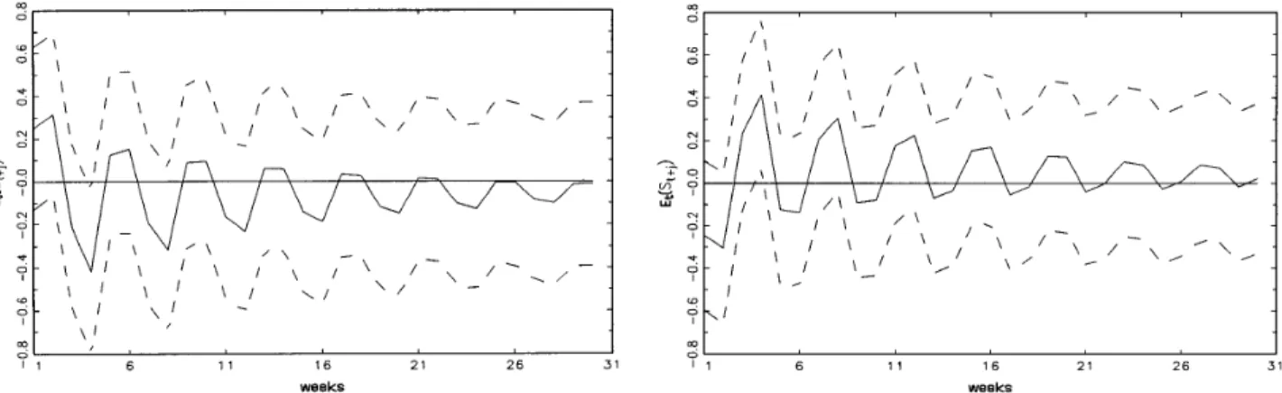
In this Appendix, we provide the confidence bands for the two key findings. The bands were constructed using the bootstrap procedure described in Gallant, Rossi, and Tauchen (1993), by refitting 300 simulated data sets from B4914210 model.4
Figures 5a and 5b show 90% confidence bands about the estimates
{ ˆV1s,j(xA+) − ˆV1s,j(xA−)}30j=1 and { ˆVf p,j(xB+) − ˆVf p,j(xB−)}j30=1,
respectively. If the population volatility function is symmetric, then the differences should be insignificant. Figure 5a shows that except for the first week, one cannot reject the null hypothesis of symmetric response of the spot volatility to interest rate differential shocks. Strong evidence is also given in Figure 5b with regard to the asymmetric response of the forward volatility to risk premium shocks: the effect to negative shocks is larger than that to positive shocks.
Figures 5c and 5d show 95% confidence bands about the estimates
{ ˆfpj(xB+) − ˆfpj(x0)}j30=1 and { ˆfpj(xB−) − ˆfpj(x0)}30j=1,
respectively, in which the cyclical response pattern of the forward premium to risk premium shocks is supported. The 95% confidence bands of the estimates
{ ˆVf p,j(xB+) − ˆVf p,j(x0)}j30=1 and { ˆVf p,j(xB−) − ˆVf p,j(x0)}30j=1,
are given in Figures 5e and 5f, respectively. For the impulse response to negative risk premium shock, the evidence of statistical significance is stronger than that to positive shock.
4The computation proceeds as follows. First, 300 data sets with the same length are generated from the estimated conditional density ˆf(y | x)
using the original initial conditions. Second, the conditional density is re-estimated from each simulated data set. Then the conditional moment profiles are computed from it. A 95% (or 90%) sup-norm confidence band is anε-band around the profile from ˆf(y | x) that is just wide enough to contain 95% (or 90%) of the 300 simulated profiles.
A, volatility response of spot rate to positive minus negative type-A shock;
B, volatility response of forward premium to positive minus negative type-B shock;
C, impulse response of forward premium to positive type-B shock relative to baseline;
D, impulse response of forward premium to negative type-B shock relative to baseline;
E, volatility response of forward premium to positive type-B shock relative to baseline;
F, volatility response of forward premium to negative type-B shock relative to baseline;
Figure 5
G, impulse response of spot rate to positive type-B shock relative to baseline; and
H, impulse response of forward premium to negative type-B shock relative to baseline.
ˆ ˆ
Figure 5
Continued.
Figures 5g and 5h show the confidence estimates of the spot response to the effects of risk-premium shock relative to baseline
{1sj(xB+) − 1sj(x0)}30j=1 and {1sˆj(xB−) − 1sˆj(x0)}j30=1.
The point estimates of deviations relative to baseline exclude or slightly include the null profile in the first few weeks, which indicate statistical significance at the 90% level.
Table 2
Bivariate SNP estimation. The Hannan-Quinn preferred model is highlighted.
Lu Lr Lp Kz Iz Kx Ix pθ sn Hannan-Quinn 0 0 1 0 0 0 0 5 2.84590 2.85321 1 0 1 0 0 0 0 9 2.63232 2.65503 2 0 1 0 0 0 0 13 2.53970 2.57250 2 3 1 0 0 0 0 19 2.49473 2.54267 2 3 1 4 4 0 0 27 2.26740 2.33553 2 3 1 4 3 0 0 27 2.25971 2.32783 2 3 1 4 2 0 0 28 2.25933 2.32999 3 0 1 0 0 0 0 17 2.50526 2.54816 4 0 1 0 0 0 0 21 2.34231 2.39530 4 4 1 0 0 0 0 29 2.28050 2.35367 4 9 1 0 0 0 0 39 2.17402 2.27243 4 9 1 4 4 0 0 47 1.92811 2.04670 4 9 1 4 2 0 0 48 1.92809 2.04921 4 9 1 4 2 1 0 68 1.87097 2.04255 5 0 1 0 0 0 0 25 2.30167 2.36475 5 1 1 0 0 0 0 27 2.27817 2.34630 5 2 1 0 0 0 0 29 2.26781 2.34099 5 3 1 0 0 0 0 31 2.25666 2.33488 5 4 1 0 0 0 0 33 2.23541 2.31868 5 5 1 0 0 0 0 35 2.20543 2.29374 5 5 1 1 0 0 0 37 2.19938 2.29274 5 5 1 1 1 0 0 37 2.19938 2.29274 5 5 1 2 2 0 0 39 2.15364 2.25205 5 5 1 3 3 0 0 41 2.15209 2.25554 5 5 1 2 2 1 0 49 2.12021 2.24385 5 5 1 2 1 1 0 49 2.12018 2.24382 5 5 1 2 0 1 0 52 2.11782 2.24903 5 5 1 2 2 2 0 64 2.08021 2.24170 5 5 1 2 1 2 0 64 2.08021 2.24170 5 5 1 2 0 2 0 70 2.07943 2.25606 5 5 2 2 0 1 0 64 2.10153 2.26302 5 5 2 2 0 2 0 124 2.02169 2.33457 5 5 1 3 2 1 0 55 2.08309 2.22187 5 5 1 3 2 1 0 55 2.08349 2.22227 5 5 1 3 1 1 0 58 2.08145 2.22780 5 5 1 3 2 1 0 55 2.08310 2.22187 5 5 1 2 0 1 0 52 2.11782 2.24903 5 6 1 0 0 0 0 37 2.19874 2.29210 5 7 1 0 0 0 0 39 2.19200 2.29040 5 8 1 0 0 0 0 41 2.18466 2.28811 5 9 1 0 0 0 0 43 2.14598 2.25448 5 9 1 1 1 0 0 45 2.14198 2.25552 5 9 1 2 2 0 0 47 2.11086 2.22945 5 9 1 3 3 0 0 49 2.10602 2.22966 5 9 1 4 4 0 0 51 1.92596 2.05464 5 9 1 4 3 0 0 51 1.92596 2.05464 5 9 1 4 2 0 0 52 1.92597 2.05718 5 9 1 4 1 0 0 54 1.92584 2.06210 5 9 1 4 2 1 0 72 1.86797 2.04964 5 9 1 4 1 1 0 78 1.86482 2.06163 5 9 1 4 0 0 0 57 1.92123 2.06505 5 9 1 4 0 1 0 87 1.85709 2.07661 5 9 1 4 0 2 0 132 1.80355 2.13662 5 9 1 4 0 2 0 132 1.80356 2.13663 6 0 1 0 0 0 0 29 2.29588 2.36905 7 0 1 0 0 0 0 33 2.29072 2.37398
Advisory Panel
Jess Benhabib, New York University
William A. Brock, University of Wisconsin-Madison Jean-Michel Grandmont, CEPREMAP-France Jose Scheinkman, University of Chicago
Halbert White, University of California-San Diego
Editorial Board
Bruce Mizrach (editor), Rutgers University Michele Boldrin, University of Carlos III Tim Bollerslev, University of Virginia
Carl Chiarella, University of Technology-Sydney W. Davis Dechert, University of Houston Paul De Grauwe, KU Leuven
David A. Hsieh, Duke University
Kenneth F. Kroner, BZW Barclays Global Investors Blake LeBaron, University of Wisconsin-Madison Stefan Mittnik, University of Kiel
Luigi Montrucchio, University of Turin Kazuo Nishimura, Kyoto University James Ramsey, New York University Pietro Reichlin, Rome University
Timo Terasvirta, Stockholm School of Economics Ruey Tsay, University of Chicago
Stanley E. Zin, Carnegie-Mellon University
Editorial Policy
The SNDE is formed in recognition that advances in statistics and dynamical systems theory may increase our understanding of economic and financial markets. The journal will seek both theoretical and applied papers that characterize and motivate nonlinear phenomena. Researchers will be encouraged to assist replication of empirical results by providing copies of data and programs online. Algorithms and rapid communications will also be published.