Adaptive Estimation and Reduction of Noises Affecting a Self-Mixing Interferometric Laser Sensor

HAL Id: hal-02959446

https://hal.laas.fr/hal-02959446

Submitted on 6 Oct 2020

HAL is a multi-disciplinary open access

archive for the deposit and dissemination of

sci-entific research documents, whether they are

pub-lished or not. The documents may come from

teaching and research institutions in France or

abroad, or from public or private research centers.

L’archive ouverte pluridisciplinaire HAL, est

destinée au dépôt et à la diffusion de documents

scientifiques de niveau recherche, publiés ou non,

émanant des établissements d’enseignement et de

recherche français ou étrangers, des laboratoires

publics ou privés.

a Self-Mixing Interferometric Laser Sensor

Zohaib Khan, Usman Zabit, Olivier Bernal, Tassadaq Hussain

To cite this version:

Zohaib Khan, Usman Zabit, Olivier Bernal, Tassadaq Hussain. Adaptive Estimation and Reduction

of Noises Affecting a Self-Mixing Interferometric Laser Sensor. IEEE Sensors Journal, Institute of

Electrical and Electronics Engineers, 2020, 20 (17), pp.9806-9815. �10.1109/JSEN.2020.2992848�.

�hal-02959446�

other works.

DOI :10.1109/JSEN.2020.2992848

1_{Department of Electrical Engineering, Riphah International University, Islamabad, 44000, Pakistan}

2_{Department of Electrical Engineering, National University of Sciences and Technology (NUST), Islamabad, 44000, Pakistan} 3_{Universite de Toulouse, LAAS-CNRS, INPT, Toulouse, 31400, France}

DOI : 10.1109/JSEN.2020.2992848

Abstract—Experimental Self-Mixing (SM) or optical feedback interferometric signals are usually affected by additive white Gaussian noise (AWGN) and impulsive noise. Depending on SM sensing set-up, these noises can significantly reduce the signal to noise ratio (SNR) of SM signals which in turn affects the measurement performance of signal processing algorithms employed for metric information retrieval. In this paper, adaptive line enhancement (ALE) technique is proposed to remove AWGN and impulsive noise from SM signals. Specifically, a recursive least squares (RLS) based ALE algorithm has been designed and the results have been compared with established methods such as high-order digital low-pass filtering and discrete wavelet transform. The comparison indicates better precision in case of use of RLS-ALE even when significant variations occur in the operating optical feedback regime and remote target velocity as well as in presence of speckle. The proposed algorithm can also estimate the SNR of SM signals belonging to weak-, moderate-, and strong-optical feedback regime with SNR ranging from 0 dB to 40 dB, with a mean absolute error of 1.35 dB and a 1.09 dB precision. Statistical analysis of noise recovered from different experimental SM signals attests the Gaussian- and impulsive-nature of noise. Thus, the proposed method also enables a simple and reliable quantitative analysis and comparison of different laser diode based SM laser sensors operating under variable optical conditions.

Index Terms— adaptive filter, noise estimation, optical feedback, self-mixing interferometry, SNR, vibration measurement.

I. Introduction

elf-mixing interferometry (SMI) or optical feedback interferometry [1]-[3] is being actively researched for velocity [4], displacement [5], distance [6], vibration [7], flow [8], profilometry [9], range-finding [10], temperature [11], and biomedical applications [12], [13] due to the compact, self-aligned, and low-cost nature of the SM instrument.

The metric performance of SMI sensors for different above-mentioned applications is highly dependent on the signal to noise ratio of SMI signal 𝑆𝑁𝑅𝑆𝑀. The experimental SMI

signal is invariably contaminated with noises originating within photonic and electronic circuitry while SMI signal’s optical feedback (OF) regime, represented by OF coupling parameter C [1], depends on optical path. Commonly, two types of noise exist in SMI signals: impulsive noise, and additive white Gaussian noise [14]. As stated in [15], phase noise in SMI is generated by both the frequency fluctuation of the laser and the target distance fluctuation. Near the SMI discontinuities (for moderate- and strong- OF regime), this phase noise can result in the presence of “impulsive noise” or “fast switching”. These noises can severely degrade SMI based measurements, e.g. by causing 1) false detection of SMI fringes and 2) incorrect normalization resulting in unwrapping errors [16]-[19].

𝑆𝑁𝑅𝑆𝑀 and bandwidth of SMI signal 𝑏𝑤𝑆𝑀 are both also

dependent on the amount of OF [20]. The signals with low 𝐶 usually have low 𝑆𝑁𝑅𝑆𝑀 and smaller 𝑏𝑤𝑆𝑀, and a significant

portion of signal may be buried in noise while the SMI signals corresponding to high OF usually have high 𝑆𝑁𝑅𝑆𝑀 and larger

𝑏𝑤𝑆𝑀. So, the detection of SMI signal’s features and

subsequent processing is easier in such SMI signals having 1 < 𝐶 < 4.6 [16]-[18].

The presence of noise in SMI system is a serious challenge for its sensing and measurement applications. So, in order to retrieve metric information from SMI signal with high accuracy, pre-processing of SMI signal is required to remove noise without distorting the actual SMI signal. Many signal processing techniques exist for noise reduction. The most common technique is digital filtering but the design of digital filters is challenging for wide-band applications as key parameters of digital filters need to be changed if the characteristics of information signal (i.e. SMI signal corresponding to remote target motion) or those of noise change over time. As spectral properties of SMI signal vary as a function of target velocity 𝑣𝑡(𝑡) and OF, so digital filters do

not provide robust noise removal [20].

Wavelet transform has also been used for the reduction of noise in SMI signal successfully [21]. Wavelet based filter effectively reduces the noise but is limited by the problem of

Adaptive Estimation and Reduction of Noises

Affecting a Self-Mixing Interferometric Laser

Sensor

Zohaib A. Khan

_{, Student Member, IEEE, Usman Zabit}

_{, Senior Member, IEEE, Olivier D.}

Bernal

_{Member, IEEE, and Tassadaq Hussain}

selection of wavelet decomposition level which needs to be varied as a function of operating OF regime and noise power. For SMI signals affected by impulsive noise, median- and Kaiser-filtering have been reported in [20]. The impulsive noise is greatly reduced by the median filter, but some residual sparkles are left at fringe-level. Kaiser filter also removes the noise effectively, but the peak values of signal are increased thereby distorting the SMI signal.

Outlier detection and myriad filter have also been proposed for removal of SMI impulsive noise [14], [22]. The outlier detection method worked well but only for SMI signal under moderate and strong regimes. The working of myriad filter depends on two key parameters i.e. linear parameter and filter window length. It requires different calibration of both parameters for removal of transient- or additive-noise.

A solution to the above-mentioned problems is adaptive filtering, which has been widely used in environments where power and bandwidth of noise varies over time. As opposed to fixed cut-off frequency based filtering, an adaptive filter adapts its frequency response (e.g. its pass-band and stop-band characteristics) by modifying the filter coefficients or weights. Adaptive filters have been used for noise reduction in communication, speech, radar, and biomedical signals [23].

With respect to SMI, active noise cancellation model (ANC) of adaptive filtering for noise reduction has been proposed in [24]. Least mean squares (LMS) algorithm of adaptive filters was used to automatically adjust the filter weights. ANC effectively reduced the noise from SMI signal, but it required reference noise signal which was derived from the driving source of LD [24]. Use of ANC model has its own limitations as extraction of reference noise signal becomes difficult in situations where noise power is low and may not be correctly detected with a sensor [24].

Therefore, in order to resolve the problems discussed above, in this paper, a single-input adaptive model is presented which can effectively reduce the noises affecting SMI signals by automatically adjusting the filter parameters while not requiring any reference noise signal. This is achieved by using adaptive linear enhancer (ALE) model of adaptive filter. ALE has effectively reduced the noise from SMI signals under large variation in both OF coupling regime as well as remote target velocity conditions. We have used the recursive least squares (RLS) algorithm for updating the ALE. The results of proposed RLS-ALE model have been compared with standard digital low pass filter and wavelet transform based processing showing better performance of RLS-ALE such that the

information signal is effectively extracted from noisy SMI signals with high precision.

In addition, RLS-ALE has also been used for simple and direct 𝑆𝑁𝑅𝑆𝑀 estimation. Usually, 𝑆𝑁𝑅𝑆𝑀 of SM velocimeter

signal is estimated by using the FFT (Fast Fourier Transform) [25], [26] to determine the SM signal spectrum which is then used to find the difference between Doppler signal’s peak value and noise-floor level. For displacement/vibration sensing, this approach may not be appropriate as the SM signal’s spectrum spreads over multiple harmonics of each of target motion’s spectral components. Another possible approach for 𝑆𝑁𝑅𝑆𝑀 estimation is the use of SMI signal’s

phase noise, based on variance of fringe discontinuity instant which can be measured by locking the oscilloscope to fringe discontinuity instant [15]. Classical formulation of 𝑆𝑁𝑅𝑆𝑀,

both for photodiode based SMI signal acquisition (PD-SM) or laser diode’s terminal voltage based SMI signal acquisition (LV-SM) has been presented in [27]. However, as can be seen in the following section, such 𝑆𝑁𝑅𝑆𝑀 estimation may not be

so straightforward for experimental SM systems because it requires the knowledge of parameters of laser diode, photodiode as well as external optical path.

In this paper, to the best of our knowledge, we present for the first time the use of RLS-ALE for direct and simple 𝑆𝑁𝑅𝑆𝑀 estimation as well. RLS-ALE enables 𝑆𝑁𝑅𝑆𝑀

estimation without prior knowledge of SMI-, optoelectronic-, or optical path based-parameters or of noise characteristics. Using the established SMI behavioral model and additive white noise, proposed RLS-ALE has estimated 𝑆𝑁𝑅𝑆𝑀 with a

mean absolute error of 1.35 dB with a precision of 1.09 dB over 𝑆𝑁𝑅𝑆𝑀 range of 0 dB to 40 dB whereas OF strength

varied from weak- to strong-feedback regime under simulated conditions. When used on noisy experimental SM signals, the proposed method enabled direct recovery of noise content whose statistical analysis attests the Gaussian and impulsive nature of corresponding noises (presented in section IV-C). A schematic block diagram of the proposed adaptive RLS-ALE based SM sensor is shown in Fig. 1. The SM sensor setup includes laser diode (LD), photodiode (PD), focusing lens (FL) and piezoelectric transducer (PZT) which acts as a vibrating target as well as reference sensor providing DPZT(t).

The paper is organized as follows. A brief introduction to SM interferometry is provided in section II. Then, the signal processing of the adaptive SM sensor is elaborated in section III. The simulated and experimental results are given in section IV, followed by Discussion and Conclusion.

II. SELF-MIXING INTERFEROMETRY

SMI phenomenon occurs in a laser when a small part of the laser light is reflected back by a target having displacement

D(t) and is fed back into the internal laser cavity. As a result,

the emitted- and reflected-light interfere with each other. This causes variation in the laser output power 𝑃(𝑡) given as [1]: 𝑃(𝑡) = 𝑃0[1 + 𝑚. cos(ϕ𝐹(𝑡))] (1)

Fig. 1. Block diagram of the adaptive noise estimation and reduction model using RLS-ALE: photodiode (PD), laser diode (LD), focusing lens (FL), and piezoelectric transducer (PZT).

other works

DOI :10.1109/JSEN.2020.2992848 where P0 is the emitted optical power without laser feedback,

m is the modulation index and ϕ F(t) is the laser output phase in the presence of feedback, given by:

ϕ𝐹(𝑡) = 2𝜋 𝐷(𝑡)

𝜆_𝐹(𝑡)/2 (2)

Under optical feedback, ϕF(t) is determined by the well-established Lang-Kobayashi model [2], given as

ϕ0(𝑡) − ϕ𝐹(𝑡) − 𝐶 sin[ϕ𝐹(𝑡) + arctan(𝛼)] = 0 (3)

where ϕ0(𝑡) is the laser output phase without the feedback,

found by replacing λF(t) with λ in (2), where λ is the LD emission wavelength in absence of feedback. α is the linewidth enhancement factor [27].

𝐶 parameter is a fundamental SMI parameter and is used to specify the SMI operating regime [29]-[31]. 𝐶 < 1 characterizes weak OF regime, and the laser output power signal varies in a quasi-sinusoidal manner. When 𝐶 > 1 then the SMI fringe shape becomes sharper, resulting in a saw-tooth like signal. As previously mentioned, spectral properties of an SMI signal (e.g. 𝑏𝑤𝑆𝑀) are a function of both OF

coupling as well as 𝑣𝑡(𝑡) (which is itself a function of target

vibration’s frequency and amplitude). For a given 𝑣𝑡(𝑡), lower

(higher) OF coupling results in lower (higher) 𝑏𝑤𝑆𝑀 [20].

𝑆𝑁𝑅𝑆𝑀 of photodiode based SMI signal acquisition (as

schematized in Fig. 1) has been formulated in [27] as 𝑆𝑁𝑅 = 2 𝐼𝑝ℎ0( 𝑡₁2 𝑟₁) 2 (𝐴 𝑒𝐵) (2𝛾𝐿 + ln 𝑅1𝑅2) −2 ₍₄₎

where R1 = r12, R2 = r22 (r1 andr2 are the field reflections at the

front- and back-mirror of LD), t1 is the fieldtransmission at the

front mirror, L is the cavity length, 𝐼𝑝ℎ0 is the photo-detected

current, B is the bandwidth of observation, e is the electron charge, 𝛾 is the power gain per unit length of the active medium, and A1/2 _{is the field attenuation suffered in}

propagation, including the diffusion at the target surface [27].

III. SIGNAL PROCESSING

The signal processing of adaptive RLS-ALE SM sensor (see Fig. 2) can be grouped into two major parts, detailed below.

A. Self-mixing Interferometric Signal:

The photodiode (PD) inside the laser diode (LD) package (see Fig. 1) is typically used to acquire the SMI signal 𝑃(𝑡).

As previously mentioned, spectral properties of an SMI signal (e.g. 𝑏𝑤𝑠𝑚) are a function of both OF coupling as well as

𝑣𝑡(𝑡) (which is itself a function of target vibration’s frequency

and amplitude). This can be verified from (1-3) indicating that higher rate of change of 𝐷(𝑡) leads to higher rate of change of 𝜙0(𝑡), 𝜙𝐹(𝑡), and 𝑃(𝑡) in the same order. The processing of

this interferometric signal leads to the reconstruction of corresponding displacement or vibration signal. To achieve accurate vibration or displacement sensing, a high-quality 𝑃(𝑡) signal is required. This paper focuses on recovering high quality P(t) by using the proposed RLS-ALE model shown in Fig. 2. The acquired noisy SMI signal is denoted as 𝑃𝑛(𝑡) =

𝑃(𝑡) + 𝑛(𝑡) where 𝑛(𝑡) denotes noise.

B. Adaptive Filtering for noise reduction:

ANC is one of the basic and mostly commonly used models for noise reduction. However, it requires a reference noise signal, which is usually not available in real-world scenarios [33], [34]. A solution to this limitation is ALE which does not require reference noise signal [23].

In the proposed ALE model, noisy SMI signal is used as the input signal as well as the reference signal (which is the same input signal but delayed by the factor Δ as shown in Fig. 2. The delayed version of noisy SMI signal 𝑃𝑛(𝑡 − 𝛥) is fed into

the adaptive filter (see Fig. 2) and filtered signal 𝑃𝑓(𝑡) is

obtained at the output, which is further processed to retrieve the displacement signal. In this paper, PUM (phase unwrapping method) [32] is used for the retrieval of displacement signal represented by 𝐷𝑟(𝑡).

1) Recursive Least Squares (RLS) Algorithm

RLS adaptive algorithm recursively updates the weights (or coefficients) of the adaptive filter so that the weighted linear least squares cost function is minimized with respect to the input signal. The RLS algorithm is known for its excellent performance while working in time varying environment but at the cost of an increased computational complexity and some stability constraints [23]. In this work, RLS-ALE requires two inputs: input noisy signal denoted as X(n) and its delayed version denoted as 𝑋(𝑛 − 𝛥) which acts as the reference noise signal. The error signal in this case is the difference between input signal and weighted reference signal given by [23]:

𝑒(𝑛) = 𝑋(𝑛) − 𝑤𝑇 𝑋(𝑛 − Δ) (5)

In our case the input signal becomes 𝑃𝑛(𝑡)as shown in the

Fig. 2. The output of adaptive filter is the weighted signal which is the filtered signal denoted by 𝑃𝑓(𝑡). RLS filter

coefficients are updated by [23]

𝑤(𝑛) = 𝑤(𝑛 − 1) + 𝑘(𝑛)𝑒(𝑛) (6) where 𝑘(𝑛) is the filter gain given by [23]

𝑘(𝑛) = Λ−1∅𝒚(𝑛−1)𝑋(𝑛−Δ)

1+Λ−1_𝑋𝑇_{(𝑛−Δ)∅𝒚(𝑛−1) 𝑋(𝑛−Δ)} (7)

where Λ is the adaptation factor, and ∅𝒚 is the correlation

matrix, and is recursively updated by [23]

∅𝒚(𝑛) = Λ−1∅𝒚(𝑛 − 1) − Λ−1𝑘(𝑛)𝑋𝑇(𝑛 − Δ)∅𝒚(𝑛 − 1) (8)

The initial value of ∅𝑦(𝑛) is equal to the product of identity

matrix 𝑰 and regularization parameter 𝛿 given by [23]

Fig. 2. Signal processing for the adaptive RLS-ALE based SM sensor: PUM (Phase Unwrapping Method) [32] is used to quantify the performance of proposed filter for displacement sensing.

∅𝒚(𝑛) = 𝛿𝑰 (9)

The stability of RLS algorithm can be controlled by 𝛿. A small positive constant number is assigned to 𝛿 for the reduction of noise from signals [23].

IV. RESULTS

Simulated and experimental SMI signals have been tested using RLS-ALE adaptive noise reduction model. Same signals have been tested by using standard LPF and DWT, and the results are compared, as detailed below.

A. Results of Simulated SMI Signals

To establish fair comparison between ALE-RLS, LPF, and DWT based filtering, different SMI specific parameters such as 𝐶, 𝛼, and target vibration frequency 𝑓𝑃𝑍𝑇 were used to cover

the usual parameter range of interest. Then, filter-specific parameters of LPF (type of filter, order of filter 𝑁𝐿𝑃𝐹, and

cut-off frequency 𝑓𝑐), and of DWT (type of wavelet, order of filter

𝑁𝐷𝑊𝑇, decomposition-level of filter 𝐿𝐷𝑊𝑇) were varied until

their corresponding error performance compared favorably with the deployed RLS-ALE based filter. Error performance of these three filtering schemes (after this optimization of LPF and DWT) is discussed below. Note that RLS-ALE filter order 𝑁𝐴𝐿𝐸 is kept constant to 150 while Δ is set to 5 in all the

cases. (𝑁𝐴𝐿𝐸 = 150 was chosen as the optimized value after

multiple simulations as lower 𝑁𝐴𝐿𝐸 gave higher measurement

error while higher 𝑁𝐴𝐿𝐸 did not improve error performance.)

Firstly, it was simulated to test if the RLS-ALE model can self-adaptively remove the noise in an SMI signal belonging to weak OF regime (𝐶 = 0.9) with λ = 0.785 µm and α=5, simulated by employing the SM behavioral model [35]. This behavioral model enables generating the SM signal 𝑃(𝑡) = cos(𝜙𝐹(𝑡)) corresponding to given 𝐷(𝑡) by solving the excess

phase equation (3) as a function of 𝐶, 𝛼, and 𝜙0(𝑡) = 4𝜋

𝜆 𝐷(𝑡).

Target vibration 𝑓𝑃𝑍𝑇 was set to 100 Hz with Ap-p =4.1 µm and

a sampling frequency of 𝑓𝑆= 100 𝑘𝐻𝑧 while 𝑆𝑁𝑅𝑆𝑀 was

12.2 dB (see Fig. 3). 𝑁𝐿𝑃𝐹 was set to 5000 while 𝑓𝑐 was set to

1 kHz, as per previously described optimization of LPF parameters required to achieve the optimum results. Similarly, Daubechies wavelet with 𝑁𝐷𝑊𝑇 = 4 was chosen for reduction

of noise (as it has similarity with the shape of SMI signal fringe [21]) while the optimum result of DWT is obtained by setting 𝐿𝐷𝑊𝑇 to 3.

To compare the performance of RLS-ALE model with LPF and DWT based filtering, the filtered SMI signals were processed by PUM [36] and the retrieved 𝐷𝑟(𝑡)l was

compared with the reference displacement signal DPZT(t). The

displacement signals recovered by using RLS-ALE, LPF and DWT shown in dotted yellow, green, and red respectively, match well with the reference DPZT(t) signal shown in blue

(see Fig. 3(f)). The error signal between reference and retrieved-displacement signal by RLS-ALE, LPF and DWT is shown in Fig. 3(g), with RMS error 𝜖𝐴𝐿𝐸 , 𝜖𝐿𝑃𝐹, and 𝜖𝐷𝑊𝑇 of

19.1 nm, 38.3 nm, and 21.3 nm, respectively.

Secondly, one of the operating (target motion) parameters (in this case 𝑓𝑃𝑍𝑇) was changed while keeping all the other

parameters the same. Fig. 4 represents the case where 𝑓𝑃𝑍𝑇=

10 𝐻𝑧 while keeping all the other parameters the same. RLS-ALE has removed the noise effectively with 𝜖𝐴𝐿𝐸= 28.5 nm.

However, LPF and DWT performance degrades with 𝜖𝐿𝑃𝐹=146 nm and 𝜖𝐷𝑊𝑇= 1952 nm. Note that the threshold

used for correct fringe detection (FD) within PUM was optimized to enable as good FD as possible for all three algorithms. However, ineffective noise reduction by LPF and DWT resulted in false FD (one incorrect fringe in case of LPF and eight incorrect fringes in case of DWT) which caused corresponding increase in measurement error.

Thirdly, Fig. 5 represents the case where 𝑓𝑃𝑍𝑇= 1kHz with

Ap-p =4.1 µm and the corresponding simulated SMI signal has

the same parameters of 𝐶=0.9, λ = 0.785 µm, and α=5 as shown in Fig. 5 (a). The sampling frequency in this case is set to 𝑓𝑆= 1 MHz. The RLS-ALE model has effectively removed

the noise without significantly distorting the shape of the SMI signal, while the LPF and DWT have also removed the noise but the shape of SMI signal is significantly distorted (indicating that significant spectral content of SMI signal has also been removed by the LPF and DWT). It is reiterated that the filter-specific parameters of LPF and DWT are kept the same as those of the first case of 𝑓𝑃𝑍𝑇= 100 𝐻𝑧 (for which

optimum error performance results were obtained). The displacement signal recovered from RLS-ALE matches well with 𝐷𝑃𝑍𝑇(𝑡), while the displacement signals recovered by

DWT and LPF deviate from 𝐷𝑃𝑍𝑇(𝑡), as quantified by the

RMS error of 𝜖𝐴𝐿𝐸 = 20.1 nm 𝜖𝐿𝑃𝐹= 2859 nm and 𝜖𝐷𝑊𝑇 =

9861 nm. The RMS error shows that the performance of LPF and DWT drastically falls because of wrongly detected fringes while RLS-ALE has maintained its performance.

Fourthly, it was simulated to test if the RLS-ALE, LPF and DWT can provide acceptable correction if 𝐶 changes (e.g. if it increases from low- to strong-OF regime) while keeping 𝑓𝑃𝑍𝑇 and all the other parameters the same.

Fig. 6 presents the case of 𝑓𝑃𝑍𝑇= 100 𝐻𝑧 and 𝐶 = 4.9, and

α=5. Again, RLS-ALE has removed the noise effectively

without distorting the shape of SM signal with 𝜖𝐴𝐿𝐸= 15.1

nm. The DWT has also removed the noise to major extend, without distorting the shape of SMI fringes, yet, presence of noise can be seen within filtered signal while the LPF has distorted the shape of SMI fringes, as quantified by 𝜖𝐿𝑃𝐹 =

3507 nm and 𝜖𝐷𝑊𝑇 = 7206 nm due to some missed fringes.

Thus, it is observed that change in 𝐶 alone (while keeping all other parameters the same) can degrade the performance of both LPF and DWT while RLS-ALE maintains its performance due to its adaptive nature.

Various other simulations were also performed by changing the value of 𝐶 and 𝑆𝑁𝑅𝑆𝑀 for 𝑓𝑃𝑍𝑇= 50 𝐻𝑧 and 𝑓𝑃𝑍𝑇=

500 𝐻𝑧 while keeping all other parameters the same. These results are summarized in Fig. 7.

B. SNR Estimation using RLS-ALE

In most experimental systems, direct and real-time access to noise is not available making it difficult to estimate the SNR of experimental signals. Proposed RLS-ALE solves this problem by not just giving the estimate of information signal (i.e.𝑃𝑓(𝑡)) but the estimate of noise residue (i.e. 𝑒(𝑡)) as well.

other works

DOI :10.1109/JSEN.2020.2992848 These estimates can then be used to estimate 𝑆𝑁𝑅𝑆𝑀 as per

𝑆𝑁𝑅 = 10𝑙𝑜𝑔10

(𝑆𝑖𝑔𝑛𝑎𝑙 𝑃𝑜𝑤𝑒𝑟)

(𝑁𝑜𝑖𝑠𝑒 𝑃𝑜𝑤𝑒𝑟) (10) Multiple simulations were conducted by varying OF strength from weak- to moderate- to strong-OF regime while 𝑆𝑁𝑅𝑆𝑀

was varied from approximately 0 dB to 40 dB (see Table I). Comparison with actual 𝑆𝑁𝑅𝑆𝑀 values shows that RLS-ALE

has estimated 𝑆𝑁𝑅𝑆𝑀 with absolute mean error and standard

deviation of 1.35 dB and 1.09 dB, respectively. This thus indicates the use of RLS-ALE as a reliable yet simple estimator of SNR for different SM sensing systems.

C. Results of Experimental SMI Signals

The experimental set-up deployed for the validation of RLS-ALE sensing model has been schematized in Fig. 1. The laser diode used for SM sensing is a Sanyo® _{DL7140 with}

λ=785 nm and output power of 50 mW. A commercial PZT actuator from Physik Instrumente (P753.2CD) served as target. This device also has a built-in capacitive feedback sensor with 2 nm resolution that served as a reference sensor for the PZT displacement DPZT(t). It thus enables error measurements between the recovered displacement signal

Dr(t) and the reference motion DPZT(t).

So, firstly, using 𝑓𝑃𝑍𝑇= 40 𝐻𝑧, a noisy SMI signal is

acquired with (PUM based) estimated 𝐶 value of 𝐶̂ = 2.3 and estimated 𝑆𝑁𝑅𝑆𝑀 of 4.83 dB (see Fig. 8(a)). In spite of poor

SNR, the ALE with 𝑁𝐴𝐿𝐸 = 150 has eliminated noise in a very

effective way without distorting the SMI signal shape significantly.

To achieve optimum results, 𝑁𝐿𝑃𝐹, 𝑓𝑐 and 𝐿𝐷𝑊𝑇 were set to

5000, 2 kHz, and 2, respectively. Thus, LPF and DWT also removed the noise successfully without distorting shape of SMI signal. The retrieved displacement signals are shown in the Fig. 8(e) with the rms errors of 𝜖𝐴𝐿𝐸 = 32.1 nm, 𝜖𝐿𝑃𝐹 =

72.3 nm and 𝜖𝐷𝑊𝑇 = 245 nm.

Then, the same experimental SMI signal was processed by using the filter parameters of LPF and DWT chosen for processing simulated SMI signals (i.e. 𝑓𝑐= 1 kHz and 𝐿𝐷𝑊𝑇

=3). Thus, one key parameter was changed in LPF and DWT to observe the corresponding effect on error performance. Expectedly, the performance of LPF and DWT is reduced if a key parameter (C, 𝑓𝑃𝑍𝑇, … ) is changed with RMS errors of

𝜖𝐿𝑃𝐹= 1787 nm and 𝜖𝐷𝑊𝑇= 728 nm respectively.

Secondly, an experimental SMI signal corresponding to dual-tone target vibration was processed (PZT was vibrating at 52 Hz and 85 Hz with Ap-p = 5 µm and Ap-p = 7 µm

respectively). The noisy SMI signal had SNR of 9.15 dB. To achieve the optimal result, 𝑁𝐿𝑃𝐹, 𝑓𝑐 and 𝐿𝐷𝑊𝑇 was adjusted to

5000, 2.5 kHz and 3, respectively. The error plots are shown in Fig. 9(e) with 𝜖𝐴𝐿𝐸 = 24.2 nm, 𝜖𝐿𝑃𝐹= 34.1 nm and

𝜖𝐷𝑊𝑇= 38.6 nm, showing the best performance of RLS-ALE

(while always using 𝑁𝐴𝐿𝐸 = 150). When the same signal was

processed by using the LPF and DWT parameters chosen for the first case (i.e. 𝑓𝑐 = 2 kHz and 𝐿𝐷𝑊𝑇 = 2), the RMS error

values increase sharply to 𝜖𝐿𝑃𝐹= 424 nm and 𝜖𝐷𝑊𝑇 = 741nm.

The above-mentioned results indicate that RLS-ALE performance remains consistent while the filter parameters of LPF and DWT need to be changed as a function of SM signal characteristics. Interestingly, even after optimization of LPF

Fig. 3.Simulation for fPZT = 100 Hz: (a) SMI signal with C= 0.9 and

α=5, (b) Noisy SM signal with SNR = 12.2 dB, (c) SM signal recovered with RLS-ALE, (d) SM signal recovered with LPF, (e) SM signal recovered with DWT, (f) Displacement Dr (t)retrieved by

PUM, (blue (reference target displacement DPZT(t) ) , yellow dotted

(RLS-ALE), red (DWT) and green (LPF), (g) Error e(t) = DPZT(t)– Dr(t) [RLS-ALE(dotted blue), LPF (green), DWT (red)].

Fig. 4.Simulation for fPZT= 10 Hz: (a) SMI signal with C= 0.9 and

α=5, (b) Noisy SM signal with SNR= 12.1 dB, (c) SM signal recovered with RLS-ALE, (d) LPF, (e) DWT, (f) Dr (t) retrieved by

PUM, blue (DPZT(t)), yellow dotted (RLS-ALE), red (DWT) and green

and DWT parameters, performance of RLS-ALE remains better (as seen in Table II which includes the error performance for other experimental SMI signals as well while using optimized LPF and DWT filter parameters).

Fig. 5.Simulation for fPZT = 1 kHz: (a) SMI signal with C= 0.9 and

α=5, (b) Noisy SM signal with SNR= 12.2 dB, (c) SM signal recovered with RLS-ALE, (d) ) LPF, (e) DWT, (f) Dr (t)retrieved by

PUM, blue (DPZT(t)), yellow dotted (RLS-ALE), red (DWT) and green

(LPF), (g) Error [RLS-ALE(dotted blue), LPF (green), DWT (red)].

Fig. 6.Simulation for fPZT = 100 Hz: (a) SMI signal with C= 4.9 and

α=5, (b) Noisy SM signal with SNR= 12.1 dB, (c) SM signal recovered with RLS-ALE, (d) LPF, (e) DWT, (f) Dr (t)retrieved by

PUM, (blue (DPZT(t)), yellow dotted (RLS-ALE), red (DWT) and

green (LPF), (g) Error [RLS-ALE(dotted blue), LPF (green), DWT (red)].

Fig. 7. PUM based RMS error results in displacement measurements of simulated SMI signals for different optical feedback, and SNR: (a) fPZT = 50Hz, and (b) fPZT = 500Hz.

TABLEI

RLS-ALE BASED SNRESTIMATION OF SIMULATED SMISIGNALS FOR DIFFERENT OPTICAL FEEDBACK AND NOISE POWER

PZT (Hz) C SNR using (10) (dB) _{RLS-ALE (dB)} SNR using Absolute Error (dB) 50 0.9 0.4 2.8 2.4 6.01 5.06 0.95 10.27 8.3 1.97 20.8 21.8 1 30.8 31.3 0.5 40.9 41.6 0.7 2.9 0.50 1.47 0.97 6.03 5.2 0.83 10.05 9.31 0.74 20.07 20.01 0.06 30.06 30.6 0.54 40.06 40.1 0.04 4.9 0.3 3.1 2.8 6.1 6.7 0.6 10.1 11.3 1.2 20.04 17.9 2.14 30.7 26.9 3.8 40.05 43.2 3.15

other works

DOI :10.1109/JSEN.2020.2992848 1) Impulsive-noise affected SMI signals

Different impulsive-noise affected SMI signals were also processed proposed RLS-ALE. Due to self-adaptive nature of RLS-ALE, good impulsive noise removal is achieved, as shown in Fig. 10, and Fig. 11. Note that Fig. 10 (a) presents an experimental SMI signal corresponding to vibration at 8 kHz with amplitude < 1µm while Fig. 11 (a) presents another SMI signal corresponding to 170 Hz vibration with 23 µm

amplitude. RLS-ALE estimated SNRSM to be 29.5 dB and 35.3

dB, respectively.

2) Speckle affected SMI signals

RLS-ALE was also tested on speckle affected SMI signal to check if it can remove noise in all or specific region of the said signal. The speckle affected SMI signals appear as amplitude modulated signals with variable 𝐶 caused by the incoherent superposition of signals reflected from the rough target surface [19]. Fig. 12 shows that RLS-ALE has eliminated both impulsive- and white-noise in an effective manner for a speckle affected SMI signal as well.

3) Current modulated SMI signals

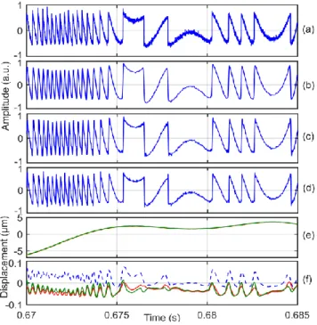
RLS-ALE was used to filter a very noisy experimental SMI signal recovered from a LD current-modulated SMI sensing set-up. Current modulation of the laser diode causes modulation of laser power which acts as a dithering signal [37]. Consequently, SMI signal is embedded within the modulated laser power (shown in Fig. 13 (a)). Recovered SMI signal is presented in Fig. 13 (b) which has been successfully de-noised by RLS-ALE with estimated 𝑆𝑁𝑅𝑆𝑀 of 2.85 dB. 4) Statistical analysis of experimental noise

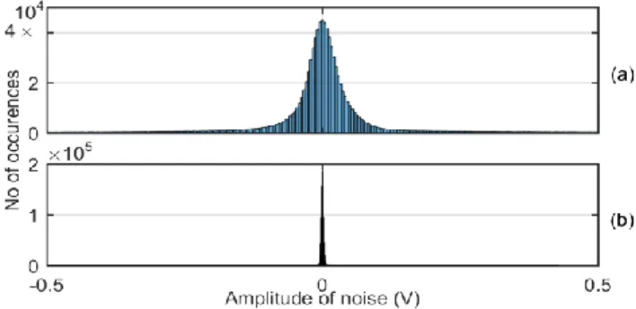
As RLS-ALE enables recovery of noise from the SM signal, so it is possible to perform statistical analysis of noise which is useful in determining the characteristics and distribution of experimental noise of a given SMI sensing set-up.

Fig. 14 (a) presents the statistical distribution of noise recovered from the SMI signal already presented in Fig. 13 (b). It can be clearly seen that this specific experimental noise satisfies the Gaussian noise model with standard deviation (𝜎) of 0.28 and mean (𝜇) of 0.00084.

Likewise, Fig. 14 (b) presents the statistical distribution of impulsive noise recovered from the SMI signal shown in Fig. 11 (a) with 𝜎 = 0.0439 and 𝜇 = -0.00041.

V. DISCUSSION

Comparison of RLS-ALE with DWT and LPF

As seen in previous results, the proposed RLS-ALE scheme is applicable on all major feedback regimes of SMI signal as well as remote-target frequency without requiring any user-driven change in filter-specific parameters.

Fig. 8.Experimental signals for fPZT = 40Hz: (a) experimental noisy

SMI signal picked up by DL7140, (b) SM signal recovered with RLS-ALE, (c) LPF, (d) DWT, (e) Dr (t)retrieved by PUM, (blue

(DPZT(t)), yellow dotted (RLS-ALE), red (DWT) and green (LPF), (f)

Error [RLS-ALE(dotted blue), LPF (green), DWT (red)].

Fig. 9. Experimental signals for fPZT= 52-85Hz: (a) experimental

noisy SMI signal picked up by DL7140, (b) SM signal recovered with RLS-ALE, (c) LPF, (d) DWT, (e) Dr (t)retrieved by PUM, (blue

(DPZT(t)), yellow dotted (RLS-ALE), red (DWT) and green (LPF), (f)

Error [RLS-ALE(dotted blue), LPF (green), DWT (red)].

Fig. 10. (a) Experimental SM signal affected by impulsive noise corresponding to vibration at 8kHz with amplitude < 1µm, (b) RLS-ALE based filtered SM signal, and (c) enlarged view of an affected fringe before and after filtering.

On the other hand, the LPF and DWT based filtering work well only under specific settings of filter-parameters, i.e., change in one of the key parameters can lead to significant degradation in performance. The key advantage of RLS-ALE is that it does not require any extraneous/additional information/input for processing noisy signals. Also, unlike other adaptive configurations, it is a single-input algorithm (i.e., no additional noise estimate/reference is needed).

Another important property of RLS-ALE which makes it superior to LPF or DWT is that it is also applicable on such SMI signals having time-varying characteristics.

In the speckle affected SMI signals with varying OF coupling, the LPF or the DWT works well for one particular signal segment but fails in other segments, while the RLS-ALE works well in all segments. The reason behind this is the fixed cut-off frequency and decomposition level of LPF and DWT, respectively. These parameters may work well for one OF regime but under-perform for other OF regime while RLS-ALE adapts itself to characteristics of SMI signal.

The main limitation of the RLS-ALE as compared to LPF and DWT is its far higher computational complexity, as seen in (5-8). RLS-ALE roughly requires 3𝑁2_{+ 11𝑁}

multiplications [23] as opposed to DWT and LPF which require 2𝑁 (per decomposition-level) and 𝑁 multiplications, respectively; where 𝑁 denotes the filter-order.

VI. CONCLUSION

An adaptive solution of de-noising SMI signal is presented which requires neither separate noise-estimation nor filter-parameter adjustments. The proposed algorithm effectively removes impulsive- and white-noise, and works wells for all major optical feedback regimes. The method is tested on both simulated- and experimental-SMI signals and the results are compared with standard LPF and DWT based filtering. This comparison shows that the proposed method provides better precision under all conditions without changing any key parameter. Noise reduction of speckle affected signals also demonstrates its robustness whereas the LPF and DWT

Fig. 11.(a) Experimental SMI signal affected by impulsive noise for multi-micrometric displacement, (b) RLS-ALE based filtered SMI signal, and (c) enlarged view of an affected fringe.

Fig. 12. (a) Experimental speckle affected signal for fPZT =110Hz:

picked up by DL7140, (b) enlarged view of red dotted block of signal in (a), (c) SM signal recovered with RLS-ALE, (d) enlarged view of pink dotted block of signal in (c).

TABLEII

PUM BASED RMS ERROR RESULTS IN THE DIPSLACEMENT MEASUREMENT OF EXPERIMENTAL SMISIGNALS FOR DIFFERENT

TARGET VIBRATIONS, OPTICAL FEEDBACK AND SNR

PZT (Hz) 𝐶̂ Estimated SNR (dB) 𝝐𝑨𝑳𝑬 (nm) 𝝐𝑳𝑷𝑭 (nm) 𝝐𝑫𝑾𝑻 (nm) 40 2.3 4.83 32.1 72.3 245 52-85 2.9 9.15 24.2 34.1 38.6 70 2.2 3.82 34 64.9 43.2 100 2.4 8.87 22.1 43.6 36.1 35-175 2.1 3.3 27.2 39.7 42.1 mean 27.9 50.9 81

Fig. 13. (a) Experimental current-modulated laser output power signal for fPZT = 10Hz with 150nm amplitude. Modulating current

signal had frequency of 100Hz, (b) recovered noisy SMI signal, and (c) RLS-ALE based filtered SMI signal.

Fig. 14. Statistical distribution of RLS-ALE based recovered experimental noise: (a) Gaussian distribution of noise of SM signal of Fig. 13 (b) with standard deviation (𝜎) of 0.28 and mean (𝜇) of 0.00084, and (b) distribution with 𝜎 = 0.0439 and 𝜇 = -0.00041 for impulsive experimental noise of SM signal of Fig. 11 (a).

other works

DOI :10.1109/JSEN.2020.2992848 excessively smoothed the SMI signal, causing false fringe

detection. Various reported results indicate that the proposed method can be very useful for pre-processing of most SMI signals acquired under typical experimental conditions.

In addition, RLS-ALE also enables simple, direct, and accurate estimation of SNR of experimental SMI signals. Very good SNR estimations, over range of 0 dB to 40 dB approximately (see Table I) validate its usefulness for SMI, an area in which simple SNR estimators are needed.

REFERENCES

[1] S. Donati, “Developing self-mixing interferometry for instrumentation and measurements”, Laser & Photon. Rev., 6: 393417, May. 2012. [2] T. Taimre, M. Nikolić, K. Bertling, Y. L. Lim, T. Bosch, and A. D.

Rakić, "Laser feedback interferometry: a tutorial on the self-mixing effect for coherent sensing," Adv. Opt. Photon, vol. 7, pp. 570-631, 2015. [3] Scalise, L.; Yanguang Yu; Giuliani, G.; Plantier, Guy; Bosch, T.,

"Self-mixing laser diode velocimetry: application to vibration and velocity measurement," Instrumentation and Measurement, IEEE Transactions

on, vol.53, no.1, pp. 223-232, Feb. 2004.

[4] Zhao, Yunhe, et al, "Self-mixing fiber ring laser velocimeter with orthogonal-beam incident system." IEEE Photonics Journal 6.2, pp. 1-11, 2014.

[5] A. Ehtesham, U. Zabit, O. D. Bernal, G. Raja and T. Bosch, "Analysis and Implementation of a Direct Phase Unwrapping Method for Displacement Measurement Using Self-Mixing Interferometry," in IEEE

Sensors Journal, vol. 17, no. 22, pp. 7425-7432, Nov. 2017.

[6] Magnani, A; Pesatori, A; Norgia, M., "Real-Time Self-Mixing Interferometer for Long Distances," Instrumentation and Measurement,

IEEE Transactions on, vol.63, no.7, pp.1804-1809, July. 2014.

[7] U. Zabit, O. D. Bernal, S. Amin, M. F. Qureshi, A. H. Khawaja and T. Bosch, "Spectral Processing of Self-Mixing Interferometric Signal Phase for Improved Vibration Sensing Under Weak- and Moderate-Feedback Regime," IEEE Sensors Journal, vol. 19, no. 23, pp. 11151-11158, 2019. [8] Ozdemir, S.K.; Ohno, I; Shinohara, S., "A Comparative Study for the Assessment on Blood Flow Measurement Using Self-Mixing Laser Speckle Interferometer," Instrumentation and Measurement, IEEE

Transactions on, vol.57, no.2, pp. 355-363, Feb. 2008.

[9] S. Donati, and G. Martini, "3D Profilometry with a Self-Mixing Interferometer: Analysis of the Speckle Error." IEEE Photonics

Technology Letters 31.7, pp. 545-548, 2019.

[10] Vogel, F.; Toulouse, B., "A low-cost medium-resolution range finder based on the self-mixing effect in a VCSEL," Instrumentation and

Measurement, IEEE Transactions on, vol.54, no. 1, pp.428-431, 2005.

[11] Zhao, Yunkun, et al, "Temperature Measurement of the Laser Cavity Based on Multi-Longitudinal Mode Laser Self-Mixing Effect." IEEE

Sensors Journal 19.12, pp. 4386-4392, 2019.

[12] Donati, S.; Norgia, M., "Self-Mixing Interferometry for Biomedical Signals Sensing," Selected Topics in Quantum Electronics, IEEE Journal

of, vol.20, no.2, pp.104-111, 2014.

[13] Y. Wei et al., “Double-path acquisition of pulse wave transit time and heartbeat using self-mixing interferometry,” Optics Communications, vol. 393, pp. 178–184, 2017.

[14] Gao, Yan & Yu, Yanguang & Xi, Jiangtao & Guo, Qinghua & Tong, Jun & Tong, Sheng., “Removing the impulsive noise contained in a self-mixing interferometry system using outlier detection”. Optical

Engineering. 53. 124108, 2014.

[15] G. Giuliani and M. Norgia, "Laser diode linewidth measurement by means of self-mixing interferometry," in IEEE Photonics Technology

Letters, vol. 12, no. 8, pp. 1028-1030, Aug. 2000.

[16] O. D. Bernal, H. C. Seat, U. Zabit, F. Surre, and T. Bosch, "Robust Detection of Non Regular Interferometric Fringes from a Self-Mixing Displacement Sensor using Bi-Wavelet Transform", IEEE Sensors

Journal, vol. 16 , No. 22, pp. 7910, 2016.

[17] A. A. Siddiqui, U. Zabit, O. D. Bernal, G. Raja, T. Bosch, "All Analog Processing of Speckle Affected Self-Mixing Interferometric Signals", IEEE Sensors Journal, vol. 17 , No. 18, pp. 5892-5899, 2017. [18] Magnani, Alessandro, Alessandro Pesatori, and Michele Norgia,

"Self-mixing vibrometer with real-time digital signal elaboration." Applied

Optics 51.21, pp. 5318-5325, 2012.

[19] Arriaga, Antonio Luna, Francis Bony, and Thierry Bosch, "Speckle-insensitive fringe detection method based on Hilbert transform for self-mixing interferometry." Applied Optics 53.30, pp. 6954-6962, 2014. [20] Y. Yu, J. Xi and J. F. Chicharo, "Improving the Performance in an

Optical feedback Self-mixing Interferometry System using Digital Signal Pre-processing," 2007 IEEE International Symposium on Intelligent

Signal Processing, pp. 1-6, 2007.

[21] Sun, Yuan & Yu, Yanguang & Xi, Jiangtao, “Wavelet Transform Based De-noising Method for Self Mixing Interferometry Signals”. Proceedings

of SPIE - The International Society for Optical Engineering. 8351. 15-.

10.1117/12.915940, 2012.

[22] Zhenghao Liu, Yanguang Yu, Yuanlong Fan, Jiangtao Xi, Qinghua Guo, and Jun Tong, "Eliminating influence of transient oscillations on a self-mixing interferometry," Optical Engineering 55(10), 104102, October. 2016

[23] Paulo S.R. Diniz, Adaptive Filtering Algorithms and Practical

Implementation. New York, USA: Springer, 2008, ch. 5.

[24] Yanguang Yu, Tiemin Mei, Jiangtao Xi, Joe F. Chicharo, Huiying Ye, and Zhao Wang, "Eliminating noises contained in sensing signals from a self-mixing laser diode", Proc. SPIE 7656, 5th International

Symposium on Advanced Optical Manufacturing and Testing Technologies: Optical Test and Measurement Technology and Equipment, 76560E, October. 2010.

[25] R. Kliese, Y. Lim, T. Bosch, and A. Rakić, "GaN laser self-mixing velocimeter for measuring slow flows," Optics Letters. 35, pp. 814-816, 2010.

[26] R. Matharu, J. Perchoux, R. Kliese, Y. Lim, and A. Rakić, "Maintaining maximum signal-to-noise ratio in uncooled vertical-cavity surface-emitting laser-based self-mixing sensors," Optics Letters. 36, pp. 3690-3692, 2011.

[27] S. Donati, "Responsivity and Noise of Self-Mixing Photodetection Schemes," in IEEE Journal of Quantum Electronics, vol. 47, no. 11, pp. 1428-1433, Nov. 2011.

[28] Kim, Cholhyon, Cholman Lee, and O. Kwonhyok, "Effect of Linewidth Enhancement Factor on Fringe in a Self-Mixing Signal and Improved Estimation of Feedback Factor in Laser Diode." IEEE Access 7 pp. 28886-28893, 2019.

[29] G. A. Acket, D. Lenstra, A. Den Boef, and B. Verbeek, "The influence of feedback intensity on longitudinal mode properties and optical noise in index-guided semiconductor lasers," Quantum Electronics, IEEE Journal of 20, pp.1163-1169, 1984.

[30] T. Taimre and A. D. Rakic, "On the nature of Acket's characteristic parameter C in semiconductor lasers," Applied Optics 53, pp. 1001-1006, 2014.

[31] Bernal, O.D.; Zabit, U.; Bosch, T, “Classification of laser Self Mixing Interferometric signal under moderate feedback,” Applied Optics, vol. 53, no. 4, pp. 702-708, 2014.

[32] C. Bes, G. Plantier and T. Bosch, “Displacement measurements using a self-mixing laser diode under moderate feedback”, Instrumentation and

Measurement, IEEE Transactions on, vol. 55, no.4, pp.1101-1105, Aug.

2006.

[33] Saeed V. Vaseghic, Advanced Digital Signal Processing and Noise

Reduction. West Sussex, UK: John Wiley & Sons Ltd, 2008, ch. 7.

[34] Peter M. Clarkson, Optimal and Adaptive Signal Processing. New York,

USA: Routledge, 2017, ch. 5.

[35] G. Plantier, C. Bes, and T. Bosch, "Behavioral Model of a Self-Mixing Laser Diode Sensor," Quantum Electronics, IEEE Journal of 41, pp. 1157-1167, 2005.

[36] T. Hussain, S. Amin, U. Zabit, O. D. Bernal, T. Bosch. , "A High Performance Real-time Interferometry Sensor System Architecture", Microprocessors and Microsystems, Vol. 64, pp. 23-33, Oct, 2018.

[37] O. D. Bernal, U. Zabit, F. Jayat and T. Bosch, "Sub-λ/2 Displacement Sensor with Nanometric Precision based on Optical Feedback Interferometry used as a Non-Uniform Event-Based Sampling System,"