Channel coding for enhanced full rate GSM

Objective performance evaluation on a large corpus of a testing speech database show that the JAPS (Joint Position and Amplitude Search) multistage search technique proposed

We used our generic search framework to instantiate a specific search solution for this task, with the explicit goal of producing reasonable results in the space of a few

Thus, although the Mixed-LSP method is less accurate than Kabal’s method [5], it is sufficient for speech coding applications using the 34-bit scalar quantizer of the CELP FS1016..

When no active speech is detected (VAD=0) the regular coder operation is switched off, and a simpler coder produces a 47-bit silence description frame which is used by the decoder

Thus, different experiments were carried out, using the EFR coder, to measure the degradation in performance introduced by different aspects of the coder, and to explore the

In the first experiment (see Section 4) the speaker identification and verification performance degradation due to the utilization of the three GSM speech coders was assessed.. In

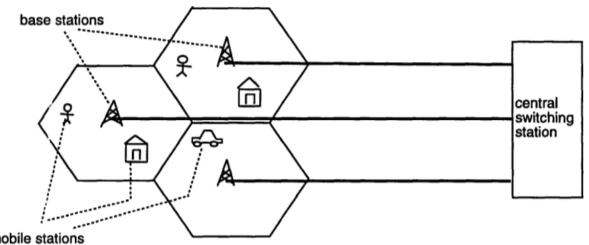
Figure 1 shows the typical speech path when a user is accessing services that requires speaker identification using his / her mobile phone.. The speech path goes from the audio input

To investigate the encoding of more complex multivariate representations of the speech stimulus and to isolate measures of multisensory integration at different