Location Prediction over Sparse User Mobility Traces Using RNNs : Flashback in Hidden States!

Location Prediction over Sparse User Mobility Traces Using RNNs:

Flashback in Hidden States!

Dingqi Yang

, Benjamin Fankhauser

, Paolo Rosso

and Philippe Cudre-Mauroux

1

_{University of Fribourg, Switzerland}

_{University of Bern, Switzerland}

_{University of Macau, SAR China}

dingqi.yang@unifr.ch, benjamin.fankhauser@students.unibe.ch, {paolo.rosso, pcm}@unifr.ch

Abstract

Location prediction is a key problem in human mo-bility modeling, which predicts a user’s next loca-tion based on historical user mobility traces. As a sequential prediction problem by nature, it has been recently studied using Recurrent Neural Net-works (RNNs). Due to the sparsity of user mo-bility traces, existing techniques strive to improve RNNs by considering spatiotemporal contexts. The most adopted scheme is to incorporate spatiotem-poral factors into the recurrent hidden state pass-ing process of RNNs uspass-ing context-parameterized transition matrices or gates. However, such a scheme oversimplifies the temporal periodicity and spatial regularity of user mobility, and thus can-not fully benefit from rich historical spatiotemporal contexts encoded in user mobility traces. Against this background, we propose Flashback, a general RNN architecture designed for modeling sparse user mobility traces by doing flashbacks on hid-den states in RNNs. Specifically, Flashback ex-plicitly uses spatiotemporal contexts to search past hidden states with high predictive power (i.e., his-torical hidden states sharing similar contexts as the current one) for location prediction, which can then directly benefit from rich spatiotemporal con-texts. Our extensive evaluation compares Flash-back against a sizable collection of state-of-the-art techniques on two real-world LBSN datasets. Re-sults show that Flashback consistently and signifi-cantly outperforms state-of-the-art RNNs involving spatiotemporal factors by 15.9% to 27.6% in the next location prediction task.

1

Introduction

User mobility modeling is one of the most important prob-lems in understanding human dynamics, which also serves as a fundamental ingredient for developing smart city applica-tions. One key task of user mobility modeling is to predict a user’s next location based on users’ historical mobility traces [Noulas et al., 2012]. Traditional methods often resort to user mobility features — either hand-crafted features such as his-torical visit counts [Noulas et al., 2012], or

automatically-learnt features using graph embedding techniques [Xie et al., 2016]) — to capture user mobility patterns. However, by gen-erating static features from historical data, these techniques predict user locations without really considering the sequen-tial patterns of user mobility, which have been shown as an important clue for location prediction [Liu et al., 2016].

Recently, Recurrent Neural Networks (RNNs) have been shown as a successful tool to model sequential data and thus started to be used also for user mobility modeling [Zhao et al., 2019]. However, classical RNN architectures, such as vanilla RNN, Long Short-Term Memory (LSTM) and Gated Recurrent Unit (GRU), were originally designed for language modeling to learn from word sequences (sentences) and they are not able to handle sparse (and incomplete) mobility traces. For example, on Foursquare, one of the most popular Loca-tion Based Social Networks (LBSNs), a user’s mobility trace is stored as a sequence of check-ins, where each check-in represents the user’s presence at a specific Point of Interests (POIs) such as a restaurant or a gym, at a specific time. As users share their check-ins on a voluntary basis on this plat-form, such mobility traces are often sparse; on our collected Foursquare dataset, we find that the average time between successive check-ins are about 59 hours. Such sparsity and incompleteness of input sequences hinders the application of RNNs to the location prediction problem [Feng et al., 2018]. To handle such sparse mobility traces, existing works strive to incorporate spatiotemporal factors into RNN architectures, as spatiotemporal contexts have indeed been shown as strong predictors for user mobility prediction [Yang et al., 2015].

In the current literature, the most popular scheme to achieve this goal is to incorporate spatiotemporal factors into the recurrent hidden state passing process of RNNs. Specifically, given a user mobility trace represented as a sequence of POIs {..., pi−1, pi, pi+1, ...}, a classical RNN

learns from the sequence by outputting a hidden state hi

from the current POI pi and the previous hidden state hi−1,

i.e., hi = F (pi, hi−1) where F (·) denotes a RNN unit

(e.g., vanilla RNN, LSTM or GRU). Subsequently, to add spatiotemporal factors, existing techniques first compute the temporal and spatial distances between the previous check-in and the current check-check-in, denoted as ∆Ti−1,i, ∆Di−1,i,

respectively, and then feed them as additional inputs to the RNN unit, i.e., hi = F (pi, hi−1, ∆Ti−1,i, ∆Di−1,i), as

Figure 1: The most popular scheme adding spatiotemporal factors into RNNs. While a classical RNN unit outputs hi= F (pi, hi−1), a

spatiotemporal RNN outputs hi= F (pi, hi−1, ∆Ti−1,i, ∆Di−1,i),

where ∆Ti−1,iand ∆Di−1,idenote the temporal and spatial

dis-tances between the previous check-in and the current check-in.

has been instantiated by either using spatiotemporal-specific transition matrices parameterized by ∆Ti−1,iand ∆Di−1,iin

RNNs [Liu et al., 2016], or extending/adding gates controlled by ∆Ti−1,i and ∆Di−1,i to LSTM [Kong and Wu, 2018;

Zhao et al., 2019]. However, this scheme cannot fully bene-fit from rich historical spatiotemporal contexts encoded in the mobility trace, due to the following reasons.

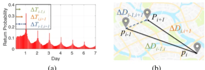
First, from a temporal perspective, feeding temporal dis-tances between successive check-ins to the RNN unit may ignore the temporal periodicity of user mobility. Specifi-cally, the periodicity of human activities is universal [Gon-zalez et al., 2008]. Figure 2(a) shows the return probabil-ity of user check-ins over time, defined as the probabilprobabil-ity of a user re-checking in at a POI a certain period of time af-ter her first check-in at that POI, on our collected Foursquare dataset. We observe a clear daily (periodic) revisiting pattern. In the context of location prediction, such a periodicity im-plies that historical check-ins with a temporal distance (taken from the current time) closer to these daily peaks (1 day, 2 days, etc.) have higher predictive power. However, iteratively feeding temporal distances between successive check-ins into the RNN unit (as shown in Figure 1) often fails to benefit from this periodicity property. Figure 2(a) illustrates such an example, where ∆Ti−1,i and ∆Ti,i+1 refers to the temporal

distances between successive check-in pairs pi−1 → pi and

pi→ pi+1, respectively. If we consider the temporal distance

in two steps (pi−1→ pi+1), we find that ∆Ti−1,i+1 is close

to the 1 day peak, indicating that pi−1is very helpful for

pre-dicting the next location. In contrast, this cannot be captured if we iteratively feed temporal distances ∆Ti−1,iand ∆Ti,i+1

into the RNN unit.

Second, from a spatial perspective, feeding spatial dis-tances between successive check-ins to the RNN unit over-simplifies the spatial regularity of user mobility. Specifically, it has been found that a user’s check-ins in a region that she frequently visited are highly biased to certain POIs [Yang et al., 2015]. In other words, those regions often have certain implicit “functions”, such as working or shopping. Subse-quently, the closer the user is to such a region, the more pre-dictable her behavior is. This suggests that the closer a past check-in is located to the current location, the more helpful it is for the next location prediction. However, only considering spatial distances between successive check-ins fails to capture such distances over space. Figure 2(b) shows an example. We observe that the spatial distance in two steps ∆Di−1,i+1

is much smaller than both ∆Di−1,i and ∆Di,i+1,

suggest-(a) (b)

Figure 2: Spatiotemporal factors in user check-in data. a) Temporal factor shown as periodicity, where the example in the box shows that considering temporal distances between successive check-ins only (∆Ti−1,iand ∆Ti,i+1) cannot capture such a periodicity. b) Spatial

factor where the example shows that considering spatial distances between successive check-ins only (∆Di−1,iand ∆Di,i+1) cannot

capture the proper distances ∆Di−1,i+1. In both cases, the

corre-sponding techniques fail to fully benefit from the historical check-ins with high predictive power when predicting location.

ing that pi−1is more helpful for location prediction. In

con-trast, this cannot be captured if we consider spatial distances ∆Di−1,iand ∆Di,i+1only.

Against this background, we propose Flashback, a general RNN architecture designed for modeling sparse user mobil-ity traces, with a particular consideration on leveraging rich historical spatiotemporal contexts by considering flashbacks on hidden states in RNNs. More precisely, departing from the widely adopted scheme of adding spatiotemporal factors into the recurrent hidden state passing process of the RNNs, our solution explicitly uses the spatiotemporal context to search past hidden states with high predictive power (i.e., histori-cal hidden states that share similar spatiotemporal contexts to the current one) for predicting the next location; as a result, our scheme can directly benefit from rich temporal (i.e, pe-riodicity as shown in Figure 2(a)) and spatial (i.e., distances over space as shown in Figure 2(b)) contexts encoded in user mobility traces. Moreover, as we do not modify the hidden state passing process of RNNs (while many existing tech-niques do), our Flashback can be easily instantiated with any RNN units (e.g., vanilla RNN, LSTM or GRU). We conduct a thorough evaluation of our method compared to a sizable collection of baselines on two real-world LBSN datasets. Re-sults show that Flashback consistently and significantly out-performs all baseline techniques. In particular, it yields an improvement of 15.9% to 27.6% over the best performing spatiotemporal RNNs.

2

Related Work

Location prediction is a key problem in human mobility mod-eling, which predicts the location of a user based on the user’s historical mobility traces. Traditional methods for location prediction often resort to various mobility features, such as hand-craft features including historical visit counts [Noulas et al., 2012; Yang et al., 2016] and activity preferences [Yang et al., 2015], or automatically-learnt features using graph em-bedding techniques [Xie et al., 2016; Yang et al., 2019]. In addition, generative/factorization models have also been used to solve location prediction/recommendation problems [Kurashima et al., 2013; Yang et al., 2013a; 2013b].

How-ever, these techniques have intrinsic limitations when captur-ing the sequential patterns of user mobility.

To capture user sequential mobility patterns, (Hidden) Markov Chains have been widely used for sequential predic-tion [Mathew et al., 2012; Cheng et al., 2013; Feng et al., 2015]. The basic idea is to estimate a transition matrix en-coding the probability of a behavior based on previous be-haviors. A typical technique here is Factorizing Personal-ized Markov Chains (FPMC) [Rendle et al., 2010], which estimates a personalized transition matrix via matrix factor-ization techniques. FPMC has been extended to the location prediction problem by further considering spatial constraints [Cheng et al., 2013; Feng et al., 2015] in building the transi-tion matrices.

Recently, Recurrent Neural Networks (RNNs) have been shown as a successful tool to model sequential data [Mikolov et al., 2010], capturing complex long- and short-term depen-dency over input sequences. To handle sparse and incom-plete sequences, existing techniques strive to add context fac-tors into the RNNs. For example, temporal facfac-tors can be added by truncating each sparse input sequence into several short sessions [Hidasi et al., 2016; Feng et al., 2018], or by considering temporal factors as additional inputs to the RNN units [Neil et al., 2016; Zhu et al., 2017]. For the problem of location prediction over sparse user mobility sequences, spatiotemporal factors have been shown as strong predictors [Yang et al., 2015]. The most popular scheme to incorporate spatiotemporal factors into RNNs is adding the spatiotempo-ral distances between (mostly successive) check-ins as addi-tional inputs to the RNN units (as illustrated in Figure 1). For example, STRNN [Liu et al., 2016] uses spatiotemporal-specific transition matrices parameterized by the spatiotem-poral distances in RNNs; HST-LSTM [Kong and Wu, 2018] extends existing gates in LSTMs to let these gates take the spatiotemporal distance as an additional input; STGN [Zhao et al., 2019] adds additional gates controlled by the spa-tiotemporal distances to LSTMs. However, as discussed in the Introduction, such schemes cannot fully benefit from the rich historical spatiotemporal contexts encoded in mobility traces. Therefore, we propose in this paper Flashback, a gen-eral RNN architecture that explicitly uses spatiotemporal con-texts to search past hidden states with high predictive power for location prediction, in order to directly benefit from the rich spatiotemporal contexts encoded in user mobility traces.

3

Flashback

Flashback is designed for modeling sparse user mobility traces, with a particular focus on leveraging rich spatiotem-poral contexts by doing flashbacks on hidden states in RNNs. Instead of implicitly considering context factors by adding spatiotemporal factors into the recurrent hidden state passing process of RNNs (as most existing techniques do), our solu-tion explicitly uses the spatiotemporal contexts to search past hidden states with high predictive power (i.e., historical hid-den states that share similar contexts as the current one) for location prediction; it can thus directly benefit from rich spa-tiotemporal contexts encoded in user mobility traces.

3.1

Overview

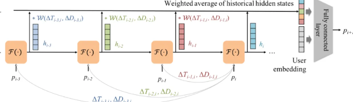
Figure 3 shows an overview of our Flashback architec-ture. Given a user’s mobility trace represented as a POI se-quence {..., pi−3, pi−2, pi−1, pi, pi+1...}, we denote the

tem-poral and spatial distances between two check-ins pi and pj

as ∆Ti,jand ∆Di,j, respectively. As shown in Figure 3, our

recurrent hidden state passing process remains unaltered from classical RNNs i.e., hi = F (pi, hi−1), letting RNNs capture

sequential user mobility patterns. However, instead of using only the current hidden state hi to predict the next location

pi+1 (as classical RNNs do), we leverage the

spatiotempo-ral context to search past hidden states with high predictive power. To achieve this goal, we compute the weighted aver-age of the historical hidden states hj, j < i, with a weight

W(∆Ti,j, ∆Di,j) as an aggregated hidden state. This weight

is parameterized by the temporal and spatial distances (∆Ti,j

and ∆Di,j, respectively) between check-in pi and pj and

measures the predictive power of the hidden state hj (more

information on this point below). Finally, in order to model individual users preferences, we define a learnable user em-bedding vector for each user, which is concatenated with the aggregated hidden state and then fed into a fully connected layer for predicting the next location, as shown in Figure 3.

In summary, to effectively predict locations from sparse user mobility traces, Flashback 1) uses RNNs to capture sequentialpatterns, 2) leverages spatiotemporal contexts to search past hidden states with high predictive power, and 3) incorporates user embeddings to consider users preferences.

3.2

Context-Aware Hidden State Weighting

The weight W(∆Ti,j, ∆Di,j) is designed to measure the

pre-dictive power of the hidden state hj according to its

spa-tiotemporal contexts.

First, from a temporal perspective, our primary goal is to incorporate the periodicity property of user behavior (as shown in Figure 2(a)) into W(∆Ti,j, ∆Di,j). Specifically,

we use a Havercosine function, a typical periodic function with outputs bounded in [0, 1], parameterized by ∆Ti,j (in

days) as follows:

wperiod(∆Ti,j) = hvc(2π∆Ti,j) (1)

where hvc(x) =1+cos(x)₂ is the Havercosine function model-ing the daily periodicity. Moreover, as we can see from Figure 2(a), the return probability exponentially decreases when in-creasing ∆Ti,j, which indicates that besides the periodicity,

the older a check-in is, the less impact it has for prediction. Subsequently, we add a temporal exponential decay weight to model this factor:

wT(∆Ti,j) = wperiod(∆Ti,j) · e−α∆Ti,j

= hvc(2π∆Ti,j) · e−α∆Ti,j

(2) where α is a temporal decay rate, controlling how fast the weight decreases over time ∆Ti,j.

Second, from a spatial perspective, we consider the fact that the closer a check-in is to the current location, the more helpful it is for location prediction (as shown in Figure 2(b)). Accordingly, we use a distance exponential decay weight to model this factor:

Figure 3: Overview of our Flashback architecture for next location prediction

Figure 4: Visualization of our proposed weight W(∆Ti,j, ∆Di,j)

over space and time. ∆Di,j is illustrated as L2 distance from the

origin over spatial space (latitude and longitude axes). We observe both a periodicity pattern over time (∆Ti,j) and a spatiotemporal

decay over space and time. The transparency of the slices on the time axis is proportional to the weights (the lower the weight is, the more transparent a slice is).

where ∆Di,jis the L2 distance between the GPS coordinates

of POIs pi and pj, and β is a spatial decay rate, controlling

how fast the weight decreases over spatial distance ∆Di,j.

Finally, we obtain the weight W(∆Ti,j, ∆Di,j) by

com-bining the temporal and spatial weights together: W(∆Ti,j, ∆Di,j) = wT(∆Ti,j) · wS(∆Di,j)

= hvc(2π∆Ti,j)e−α∆Ti,je−β∆Di,j

(4) where the first Havercosine term captures the periodicity property of user check-ins, and the exponential terms model the spatiotemporal decay of the impact of historical check-ins on location prediction. Figure 4 offers a visualization of the weights over space and time.

3.3

Discussions

Why Does Flashback Work?

By flashing back to the historical hidden states, our Flashback can discount the “noise” from the recurrent hidden state pass-ing process of the RNNs over sparse user mobility traces, and also create an explicit “attention” mechanism by leveraging past hidden states with high predictive power (i.e., historical hidden states that share similar contexts as the current hidden state) for location prediction. Figure 5 shows a toy exam-ple from the temporal perspective. On one hand, Figure 5(a) shows an actual (complete) user mobility trace with a clear se-quential pattern (“Home-Office-Restaurant-Office-Shopping-Bar-Home”), where classical RNNs can effectively capture such a pattern and predict the next location “Home”. On the

(a) Actual (complete) user mobility trace

(b) Observed (sparse) user mobility trace

Figure 5: A toy example illustrating the working principle of Flash-back from a temporal perspective.

other hand, for an observed (sparse) user mobility trace as shown in Figure 5(b), the sequential pattern is difficult to be captured by RNNs, where the hidden state passing process becomes noisy due to the incompleteness of the sequence. Even when considering temporal distances between succes-sive check-ins as additional inputs of the RNN units (as many state-of-the-art techniques do), it still falls short in capturing long-term temporal (i.e, periodicity) dependencies. However, by flashing back to the historical hidden states sharing a sim-ilar temporal context as the current one (∆T ≈ 1 day captur-ing the daily periodicity, i.e., at the similar time on the previ-ous day), Flashback can predict the next location “Home”. How Far to Flash Back?

As Flashback generates an aggregated hidden state from past hidden states, an immediate question here is how many past hidden states should be considered?To answer this question, we review the temporal exponential decay term e−α∆Ti,j _in W(∆Ti,j, ∆Di,j). Let ∆t denote the average time between

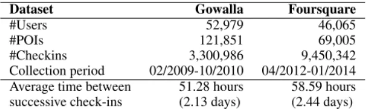
successive check-ins. The hidden state k-step back has an average ∆T = ∆t · k, corresponding to a temporal exponen-tial decay term e−α∆t·k. In practice, our empirical analysis shows that the average time between successive check-ins ∆t are 51.28 (2.13 days) hours and 58.59 hours (2.44 days) on our Gowalla and Foursquare datasets, respectively (see Sec-tion 4.1), and the optimal temporal decay rate is 0.1 in our experiments on both datasets (see Section 4.3). Therefore, the temporal exponential decay term becomes a function of k. When setting k = 20 for example, this term is around

Dataset Gowalla Foursquare

#Users 52,979 46,065

#POIs 121,851 69,005

#Checkins 3,300,986 9,450,342 Collection period 02/2009-10/2010 04/2012-01/2014 Average time between

successive check-ins

51.28 hours (2.13 days)

58.59 hours (2.44 days) Table 1: Statistics of the datasets

0.01, which is indeed the upper bound of W(∆Ti,j, ∆Di,j)

as all other terms in W(∆Ti,j, ∆Di,j) are bound to [0, 1]. In

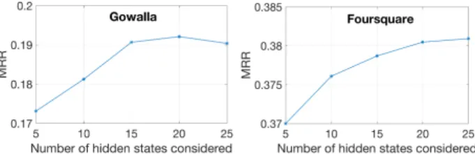
other words, a hidden state more than k-step back receives on average a weight less than 0.01, which contributes little to the aggregated hidden state. We also study this point in our experiments, where prediction performance flattens out when k ≥ 20 (see Section 4.4).

4

Experiments

4.1

Experimental Setup

Dataset

We conduct experiments on two widely used check-in datasets collected from two LBSNs: Gowalla and Foursquare, respectively. Table 1 shows the statistics of the datasets. We chronologically split all the mobility traces into 80% for train-ing and 20% for test.

Baselines

We compare Flashback against a sizable collection of state-of-the-art techniques from five categories:

• User Preference-based Methods: 1) WRMF [Hu et al., 2008] learns user preferences on POIs using matrix fac-torization; 2) BPR [Rendle et al., 2009] learns user prefer-ences on POIs by minimizing a pairwise ranking loss. • Feature-based methods: 1) Most Frequent Time (MFT,

the best-performing feature by [Gao et al., 2012]) ranks a POI according to a user’s historical check-in count at a POI and at a specific time slot (24 hours in a day) in the training dataset; 2) LBSN2Vec [Yang et al., 2019] learns user, time and POI feature vectors from a LBSN hyper-graph, and ranks a POI according to its similarities with user and time in the feature space.

• Markov-Chain-based Methods: 1) FPMC [Rendle et al., 2010] estimates a personalized transition matrix via ma-trix factorization techniques; 2) PRME [Feng et al., 2015] learns user and POI embeddings to capture the personal-ized POI transition patterns. 3) TribeFlow [Figueiredo et al., 2016] uses a semi-Markov chain model to capture the transition matrix over a latent environment.

• Basic RNNs: 1) RNN [Zhang et al., 2014] is a vanilla RNN achitecture; 2) LSTM [Hochreiter and Schmidhuber, 1997] is capable of learning long-term dependency using a memory cell and multiplicative gates; 3) GRU [Cho et al., 2014] captures long-term dependency by controlling infor-mation flow with two gates.

• Spatiotemporal RNNs: 1) DeepMove [Feng et al., 2018] adds an attention mechanism to GRU for location predic-tion over sparse mobility traces; 2) STRNN [Liu et al.,

2016] uses customized transition matrices parameterized by the spatiotemporal distances between check-ins within a time window in RNNs; 3) STGN [Zhao et al., 2019] add additional gates controlled by the spatiotemporal distances between successive check-ins to LSTM, while STGCN is a variant of STGN with coupled input and forget gates for improved efficiency.

For our proposed Flashback, as it does not depend on any specific RNN units, we instantiate it using all the three ba-sic RNNs, named as Flashback (RNN), Flashback (LSTM), and Flashback (GRU). We train Flashback by backpropaga-tion through time using the Adam stochastic optimizer with cross entropy loss. We implement Flashback in PyTorch, and our code and datasets are available here1_.

Evaluation Protocol and Metrics

We evaluate Flashback in the next location prediction task, where we predict where a user will go next, given a sequence of her historical check-ins, as shown in Figure 3. We report two widely used metrics for location prediction: average Ac-curacy@N (Acc@N), where N = 1, 5, 10, and Mean Re-ciprocal Rank (MRR). We empirically set the dimension of hidden states and all (POI and user) embedding size as 10 for all RNN-based techniques. We search the optimal temporal and spatial decay rate (α and β, respectively) on a log scale (see Section 4.3 for more details).

4.2

Location Prediction Performance

Table 2 shows the results on both Gowalla and Foursquare. In general, we observe that Flashback consistently and sig-nificantly outperforms all baseline techniques. In particular, compared to the best-performing baselines (spatiotemporal RNNs in most cases), Flashback shows an improvement of 27.7% and 15.9% in MRR, on Gowalla and Foursquare, re-spectively.

In addition, compared to the basic RNNs, Flashback con-sistently yields significant improvements of at least 27.5%, showing the effectiveness of leveraging past hidden states for next location prediction. Interestingly, we also observe a large variation on the performance of basic RNN, LSTM, and GRU (e.g., we see an MRR of 0.1507, 0.1144 and 0.0993 on the Gowalla dataset, respectively), showing their different capacities of modeling sparse user mobility traces. However, despite their different modeling capacities, Flashback imple-mented with RNN, LSTM, and GRU has a much smaller vari-ation in terms of its performance (with an MRR of 0.1925, 0.1778 and 0.1731 on Gowalla, respectively). Such an ob-servation shows that Flashback can boost the performance of any basic RNNs to a maximum extent, by fully benefiting from rich historical spatiotemporal contexts.

4.3

Impact of Spatiotemporal Decay Rates

In this experiment, we evaluate the impact of the temporal and spatial decay factors (α and β, respectively) on location pre-diction by varying α and β on a log scale. Figure 6 shows the results. On one hand, when increasing the spatial decay factor β, we observe that the prediction performance increases, and

1

Method Gowalla Foursquare

Acc@1 Acc@5 Acc@10 MRR Acc@1 Acc@5 Acc@10 MRR User Preference based Methods WRMF 0.0112 0.0260 0.0367 0.0178 0.0278 0.0619 0.0821 0.0427 BPR 0.0131 0.0363 0.0539 0.0235 0.0315 0.0828 0.1143 0.0538 Feature-based Methods MFT 0.0525 0.0948 0.1052 0.0717 0.1945 0.2692 0.2788 0.2285 LBSN2Vec 0.0864 0.1186 0.1390 0.1032 0.2190 0.3955 0.4621 0.2781 Markov-Chain based Methods FPMC 0.0479 0.1668 0.2411 0.1126 0.0753 0.2384 0.3348 0.1578 PRME 0.0740 0.2146 0.2899 0.1503 0.0982 0.3167 0.4064 0.2040 TribeFlow 0.0256 0.0723 0.1143 0.0583 0.0297 0.0832 0.1239 0.0645 Basic RNNs RNN 0.0881 0.2140 0.2717 0.1507 0.1824 0.4334 0.5237 0.2984 LSTM 0.0621 0.1637 0.2182 0.1144 0.1144 0.2949 0.3761 0.2018 GRU 0.0528 0.1416 0.1915 0.0993 0.0606 0.1797 0.2574 0.1245 Spatiotemporal RNNs DeepMove* 0.0625 0.1304 0.1594 0.0982 0.2400 0.4319 0.4742 0.3270 STRNN 0.0900 0.2120 0.2730 0.1508 0.2290 0.4310 0.5050 0.3248 STGN 0.0624 0.1586 0.2104 0.1125 0.2094 0.4734 0.5470 0.3283 STGCN 0.0546 0.1440 0.1932 0.1017 0.1878 0.4502 0.5329 0.3062 Flashback Flashback (RNN) 0.1158 0.2754 0.3479 0.1925 0.2496 0.5399 0.6236 0.3805 Flashback (LSTM) 0.1024 0.2575 0.3317 0.1778 0.2398 0.5169 0.6014 0.3654 Flashback (GRU) 0.0979 0.2526 0.3267 0.1731 0.2375 0.5154 0.6003 0.3631

Table 2: Location Prediction Performance on both Gowalla and Foursquare. The best-performing baselines and Flashback are highlighted. (*Experiments of DeepMove are conducted on 5,000 randomly sampled users, due to its poor efficiency where it takes more than one day per epoch using an NVIDIA V100 GPU for all users on both of our datasets.)

Figure 6: Impact of temporal and spatial decay rate (α and β, re-spectively)

then flattens out after β = 100 (on Foursquare) or β = 1000 (on Gowalla). This observation verifies the fact that the spa-tial distance is a very important factor defining context simi-larity for next location prediction problem; with a large β, the context similarity decreases fast with increasing spatial dis-tances2. On the other hand, when decreasing temporal decay factor α, the prediction performance slightly increases, and achieves the best performance at α = 0.1, implying a slow temporal decay over time which allows the hidden states at the periodicity peak to contribute more to location prediction. In other words, a low value of α indeed shows that the peri-odicity helps for predicting the next location.

4.4

How Far to Flash Back?

In this experiment, we study the impact of the number of in-volved past hidden states k (when flashing back) on the per-formance of location prediction. Figure 7 shows the results. We observe that performance increases with increasing k, as more hidden states can better help location prediction. The performance flattens out after k ≥ 20, as further hidden states have little contribution due to the temporal decay, which cor-responds to our previous discussion in Section 3.3.

2

We compute spatial distance ∆D using the L2 distance (in kilo-meters) between the GPS coordinates of two POIs.

Figure 7: Impact of the number of involved past hidden states k when flashing back

5

Conclusion

In this paper, we propose Flashback, a general RNN archi-tecture designed for modeling sparse user mobility traces by leveraging rich spatiotemporal contexts. Specifically, instead of implicitly considering context factors by adding spatiotem-poral factors into the recurrent hidden state passing process of RNNs (as most existing techniques do), our solution ex-plicitly uses the spatiotemporal contexts to search past hid-den states with high predictive power (i.e., historical hidhid-den states that share similar contexts as the current hidden state) for location prediction; subsequently, Flashback can directly benefit from rich spatiotemporal contexts encoded in user mo-bility traces. Our extensive evaluation compares Flashback against a sizable collection of state-of-the-art techniques on two real-world LBSN datasets. The results show that Flash-back consistently and significantly outperforms state-of-the-art spatiotemporal RNNs by 15.9% to 27.6% when tackling the next location prediction task.

In future work, we plan to incorporate learnable spatiotem-poral decay rates to fully automate our learning process.

Acknowledgements

This project has received funding from the European Re-search Council (ERC) under the European Union’s Horizon 2020 research and innovation programme (grant agreement 683253/GraphInt).

References

[Cheng et al., 2013] Chen Cheng, Haiqin Yang, Michael R Lyu, and Irwin King. Where you like to go next: Succes-sive point-of-interest recommendation. In IJCAI, 2013. [Cho et al., 2014] Kyunghyun Cho, Bart Van Merri¨enboer,

Caglar Gulcehre, Dzmitry Bahdanau, Fethi Bougares, Holger Schwenk, and Yoshua Bengio. Learning phrase representations using rnn encoder-decoder for statistical machine translation. arXiv:1406.1078, 2014.

[Feng et al., 2015] Shanshan Feng, Xutao Li, Yifeng Zeng, Gao Cong, Yeow Meng Chee, and Quan Yuan. Person-alized ranking metric embedding for next new poi recom-mendation. In IJCAI, 2015.

[Feng et al., 2018] Jie Feng, Yong Li, Chao Zhang, Funing Sun, Fanchao Meng, Ang Guo, and Depeng Jin. Deep-move: Predicting human mobility with attentional recur-rent networks. In WWW, pages 1459–1468, 2018. [Figueiredo et al., 2016] Flavio Figueiredo, Bruno Ribeiro,

Jussara M Almeida, and Christos Faloutsos. Tribeflow: Mining & predicting user trajectories. In WWW, pages 695–706, 2016.

[Gao et al., 2012] Huiji Gao, Jiliang Tang, and Huan Liu. Exploring social-historical ties on location-based social networks. In ICWSM, 2012.

[Gonzalez et al., 2008] Marta C Gonzalez, Cesar A Hidalgo, and Albert-Laszlo Barabasi. Understanding individual hu-man mobility patterns. Nature, 453(7196):779, 2008. [Hidasi et al., 2016] Bal´azs Hidasi, Alexandros

Karat-zoglou, Linas Baltrunas, and Domonkos Tikk. Session-based recommendations with recurrent neural networks. In ICLR, 2016.

[Hochreiter and Schmidhuber, 1997] Sepp Hochreiter and J¨urgen Schmidhuber. Long short-term memory. Neural computation, 9(8):1735–1780, 1997.

[Hu et al., 2008] Yifan Hu, Yehuda Koren, and Chris Volin-sky. Collaborative filtering for implicit feedback datasets. In ICDM, pages 263–272. Ieee, 2008.

[Kong and Wu, 2018] Dejiang Kong and Fei Wu. Hst-lstm: A hierarchical spatial-temporal long-short term memory network for location prediction. In IJCAI, pages 2341– 2347, 2018.

[Kurashima et al., 2013] Takeshi Kurashima, Tomoharu Iwata, Takahide Hoshide, Noriko Takaya, and Ko Fu-jimura. Geo topic model: joint modeling of user’s activity area and interests for location recommendation. In WSDM, pages 375–384. ACM, 2013.

[Liu et al., 2016] Qiang Liu, Shu Wu, Liang Wang, and Tie-niu Tan. Predicting the next location: A recurrent model with spatial and temporal contexts. In AAAI, 2016. [Mathew et al., 2012] Wesley Mathew, Ruben Raposo, and

Bruno Martins. Predicting future locations with hidden markov models. In UbiComp, pages 911–918. ACM, 2012.

[Mikolov et al., 2010] Tom´aˇs Mikolov, Martin Karafi´at, Luk´aˇs Burget, Jan ˇCernock`y, and Sanjeev Khudanpur. Re-current neural network based language model. In INTER-SPEECH, 2010.

[Neil et al., 2016] Daniel Neil, Michael Pfeiffer, and Shih-Chii Liu. Phased lstm: Accelerating recurrent network training for long or event-based sequences. In NIPS, pages 3882–3890, 2016.

[Noulas et al., 2012] Anastasios Noulas, Salvatore Scellato, Neal Lathia, and Cecilia Mascolo. Mining user mobil-ity features for next place prediction in location-based ser-vices. In ICDM, pages 1038–1043. IEEE, 2012.

[Rendle et al., 2009] Steffen Rendle, Christoph Freuden-thaler, Zeno Gantner, and Lars Schmidt-Thieme. Bpr: Bayesian personalized ranking from implicit feedback. In UAI, pages 452–461. AUAI Press, 2009.

[Rendle et al., 2010] Steffen Rendle, Christoph Freuden-thaler, and Lars Schmidt-Thieme. Factorizing personal-ized markov chains for next-basket recommendation. In WWW, pages 811–820. ACM, 2010.

[Xie et al., 2016] Min Xie, Hongzhi Yin, Hao Wang, Fan-jiang Xu, Weitong Chen, and Sen Wang. Learning graph-based poi embedding for location-graph-based recommendation. In CIKM, pages 15–24. ACM, 2016.

[Yang et al., 2013a] Dingqi Yang, Daqing Zhang, Zhiyong Yu, and Zhu Wang. A sentiment-enhanced personalized location recommendation system. In HT, 2013.

[Yang et al., 2013b] Dingqi Yang, Daqing Zhang, Zhiyong Yu, and Zhiwen Yu. Fine-grained preference-aware lo-cation search leveraging crowdsourced digital footprints from lbsns. In UbiComp, pages 479–488, 2013.

[Yang et al., 2015] Dingqi Yang, Daqing Zhang, Vincent W Zheng, and Zhiyong Yu. Modeling user activity preference by leveraging user spatial temporal characteristics in lbsns. TSMC, 45(1):129–142, 2015.

[Yang et al., 2016] Dingqi Yang, Bin Li, and Philippe Cudr´e-Mauroux. Poisketch: Semantic place labeling over user activity streams. In IJCAI, pages 2697–2703, 2016. [Yang et al., 2019] Dingqi Yang, Bingqing Qu, Jie Yang, and

Philippe Cudre-Mauroux. Revisiting user mobility and so-cial relationships in lbsns: a hypergraph embedding ap-proach. In WWW, pages 2147–2157. ACM, 2019. [Zhang et al., 2014] Yuyu Zhang, Hanjun Dai, Chang Xu,

Jun Feng, Taifeng Wang, Jiang Bian, Bin Wang, and Tie-Yan Liu. Sequential click prediction for sponsored search with recurrent neural networks. In AAAI, 2014.

[Zhao et al., 2019] Pengpeng Zhao, Haifeng Zhu, Yanchi Liu, Jiajie Xu, Zhixu Li, Fuzhen Zhuang, Victor S Sheng, and Xiaofang Zhou. Where to go next: A spatio-temporal gated network for next poi recommendation. In AAAI, vol-ume 33, pages 5877–5884, 2019.

[Zhu et al., 2017] Yu Zhu, Hao Li, Yikang Liao, Beidou Wang, Ziyu Guan, Haifeng Liu, and Deng Cai. What to do next: Modeling user behaviors by time-lstm. In IJCAI, pages 3602–3608, 2017.