Chance-constrained Scheduling via
Conflict-directed Risk Allocation
The MIT Faculty has made this article openly available.
Please share
how this access benefits you. Your story matters.
Citation
Wang, Andrew J., and Brian C. Williams. "Chance-constrained
Scheduling via Conflict-directed Risk Allocation." in Twenty-Ninth
AAAI Conference on Artificial Intelligence (AAAI-15), January, 25-30,
2015, Austin, Texas, USA.
As Published
http://www.aaai.org/Conferences/AAAI/2015/aaai15schedule.pdf
Publisher
Association for the Advancement of Artificial Intelligence
Version
Author's final manuscript
Citable link
http://hdl.handle.net/1721.1/92982
Terms of Use
Creative Commons Attribution-Noncommercial-Share Alike
Chance-constrained Scheduling via Conflict-directed Risk Allocation
Andrew J. Wang and Brian C. Williams
Computer Science and Artificial Intelligence LaboratoryMassachusetts Institute of Technology {wangaj, williams}@mit.edu
Abstract
Temporal uncertainty in large-scale logistics forces one to trade off between lost efficiency through built-in slack and costly replanning when deadlines are missed. Due to the dif-ficulty of reasoning about such likelihoods and consequences, a computational framework is needed to quantify and bound the risk of violating scheduling requirements. This work ad-dresses the chance-constrained scheduling problem, where actions’ durations are modeled probabilistically. Our solution method uses conflict-directed risk allocation to efficiently compute a scheduling policy. The key insight, compared to previous work in probabilistic scheduling, is to decouple the reasoning about temporal and risk constraints. This de-composes the problem into a separate master and subprob-lem, which can be iteratively solved much quicker. Through a set of simulated car-sharing scenarios, it is empirically shown that conflict-directed risk allocation computes solu-tions nearly an order of magnitude faster than prior art does, which considers all constraints in a single lump-sum opti-mization.
Introduction
Scheduling requirements for plans are often given as con-crete constraints: a product needs to be delivered to a cus-tomer by the end of the month; to catch the bus, one has to be at the bus stop before the bus arrives. Yet, real-world actions have uncertain durations, whether due to variabil-ity in execution or impreciseness in modeling. This uncer-tainty makes it difficult to meet the scheduling requirements with absolute certainty. However, even though uncertainty can lead to failure, the user will want to evaluate and have a guarantee on the probability of success.
This need is addressed by solving the chance-constrained scheduling problem: given a temporally flexible plan, find a scheduling policy for it that obeys the requirements within user-specified acceptable risk. Framing the problem in a probabilistic setting acknowledges that compliance under 100 percent of the scenarios may not be possible. Instead, the problem imposes well-defined limits on risk across the plan, called chance constraints. A plan’s scheduling during execution is determined by a scheduling policy; hence, the
Copyright c 2015, Association for the Advancement of Artificial Intelligence (www.aaai.org). All rights reserved.
task is to select and evaluate a policy against the problem’s chance constraints.
Prior art in scheduling with probabilistic temporal un-certainty has led to the synthesis of three key ideas: risk allocation, STNU controllability, and nonlinear constraint programming. (Tsamardinos 2002) was the first to use constraint programming to minimize temporal risk, which is a nonlinear objective. Recent work by (Fang, Yu, and Williams 2014) introduces a chance-constrained alternative that generates less conservative solutions by encoding risk allocation and STNU controllability conditions into a con-straint program. The main deficiency of these methods is that their constraint programs become large and time-consuming to solve. Off-the-shelf solvers typically use se-quential quadratic programming (Gill, Murray, and Saun-ders 2002) or interior point methods (W¨achter and Biegler 2006), whose runtimes grow polynomially in program size.
This work’s key insight, then, is to apply iterative con-flict discovery on top of the previous three ideas, so that one solves a series of constraint programs which start small and grow incrementally. The combined runtime of solving these small programs is still faster than solving one large program. This is achieved through a master-and-subproblem architec-ture that decouples the reasoning about risk and temporal constraints: First, the master generates a candidate risk allo-cation that distributes the available risk bounds across activ-ity durations, thus ensuring that the chance constraints are not violated. The risk allocation places concrete bounds on the uncertain durations, which reformulates the probabilis-tic problem into a determinisprobabilis-tic form, modeled as an STNU (simple temporal network with uncertainty). Then, the sub-problem checks the STNU for temporal controllability, and it returns temporal conflicts to be added to the master prob-lem. One repeats until there are no more conflicts, or the master deems the problem infeasible. This process is effi-cient because not all temporal constraints have to be consid-ered in generating a solution, but only in checking it.
In addition to conflict-driven risk allocation, another new feature of this work is the ability to accommodate multiple chance constraints. Each chance constraint may be defined over a subset of the entire plan. This allows users to weight the relative importance of different parts of the plan by as-signing tighter chance constraints to the more critical areas. This work’s approach is empirically validated against
the previous risk-minimizing and chance-constrained ap-proaches. In scheduling a set of simulated car-sharing sce-narios, the conflict-directed approach significantly outper-forms these two precedents in runtime. Only a negligible portion of the runtime is spent by the subproblem finding conflicts, so the runtime savings are largely attributed to solving much smaller optimizations for the master problem.
Background
This section briefly reviews temporal network concepts ref-erenced later. Namely, the STN, STNU, and pSTN for-malisms are covered. Each is a type of constraint network, and therefore has a corresponding notion of consistency.
Simple temporal networks (STNs) model the temporal structure of plans for scheduling purposes (Dechter, Meiri, and Pearl 1991). An STN N is a collection of events E and simple temporal constraints T . For semantic purposes, the constraints may be further divided into user-specified re-quirements Trand actions’ durations Tc. The superscript c
refers to the modeling assumption that those events and du-rations are controllable by the scheduler. Simple temporal constraints in both Trand Tc have the same form: an in-terval bound [l, u] between two events. The lower and upper bounds of the interval may be open at −∞ and +∞, respec-tively. A schedule s : E 7→ R assigns timepoints to all the events. An STN is consistent if there exists a schedule that violates no constraint. Such a schedule is also said to be consistent.
STNs may be extended to simple temporal networks with uncertainty (STNUs) to account for actions with uncontrol-lable durations (Vidal and Fargier 1999). In an STNU Nu, in addition to actions with controllable durations Tc, some actions have uncontrollable durations Tu. Uncontrollable
durations are constraints on Nature, and out of the sched-uler’s control. Like simple temporal constraints, they are also bounded by intervals, though they must be nonnegative. If an event marks the end of an uncontrollable duration, it is necessarily uncontrollable, i.e., assigned by Nature. There-fore, the set of events E is also divided into a controllable set Ecand an uncontrollable set Eu.
Given an STNU, one needs to schedule it regardless of what Nature chooses within the uncertainty specified in the uncontrollable durations. If one can schedule all the con-trollable events of an STNU, such that for any assignment to the uncontrollable events by Nature, the STNU’s tempo-ral constraints are still obeyed, then the STNU is control-lable. Controllability depends on whether the scheduling policy is determined offline or online. Strong controllabil-ity concerns offline scheduling, which must guarantee exis-tence of a static schedule that would be consistent with any outcome of the uncontrollable durations. Dynamic control-lability concerns online scheduling, where events are sched-uled with the flexibility of knowing past outcomes.
Finally, probabilistic analogue of the STNU is a prob-abilistic simple temporal network (pSTN), which models probabilistic durations (Tsamardinos 2002) (Fang, Yu, and Williams 2014). This is the representation considered in this work. A pSTN Nppreserves STNU semantics, but replaces
the uncontrollable durations Tuwith probabilistic ones Tp.
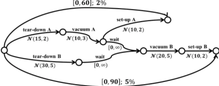
Figure 1: A chance-constrained pSTN for the room setup example.
A probabilistic duration is sampled from a temporal distri-bution over the domain [0, +∞), with pdf f and cdf F . Be-cause a pSTN’s distributions may always extend to +∞, albeit with small probability, the STNU notion of control-lability under all conditions will always fail. Therefore, a probabilistic notion of temporal controllability is needed for pSTNs.
Problem Statement
Previously, (Tsamardinos 2002) and (Fang, Yu, and Williams 2014) have established their own problem formu-lations for probabilistic scheduling. (Tsamardinos 2002) is concerned with finding a schedule that minimizes the global temporal risk of violating any constraint. In contrast, (Fang, Yu, and Williams 2014) adopts a chance-constrained formu-lation, which bounds the schedule’s temporal risk, and in-stead optimizes a separate objective expressed in terms of the resulting schedule.
This work’s problem statement differs and expands on theirs in some ways. Most importantly, although this prob-lem is also chance-constrained, multiple chance constraints may be specified over subplans, instead of a single global chance constraint over the entire plan. This allows the user to attribute different risk priorities to different parts of the plan, which is useful for large and complex scenarios. It also gives the solution method flexibility to just meet the chance constraints, rather than having to minimize a single global risk metric. In addition, while the previous two works try to find a fully grounded schedule, this work merely guarantees the existence of one through a scheduling policy, and leaves the dispatcher flexibility in determining the actual schedule. A grounded example will illustrate this work’s problem statement: Imagine a hotel management preparing two sem-inar rooms for upcoming session talks. Room A needs to be ready in one hour, and room B in one-and-half. Figure 1 diagrams a plan for setting up the rooms, along with their deadlines, in pSTN form. Each room is first cleared of fur-niture, so that it may be vacuumed, and then installed with new furniture for its session. There is only one working vac-uum, and room A gets to use it first.
Each activity in the plan has a duration associated with it. If uncontrollable, it is modeled by a normal distribution N (µ, σ). Technically, each N would be truncated below 0 renormalized, because real activities may not have negative duration. If the duration is controllable, it is modeled as a
simple temporal constraint, such as the two [0, +∞) waits. The rooms’ deadlines are also expressed as simple tempo-ral constraints. Each has a chance constraint defined over it: a maximum of two percent risk for room A’s deadline, and five percent for room B’s. Thus, A’s deadline is more im-portant, and the solution may be biased towards satisfying it over B’s.
Note that only the three activities “tear-down A”, “vac-uum A”, and “set-up A” are relevant to meeting room A’s deadline; there is no dependence on how long B’s activities take. On the other hand, because B has to wait for A to finish vacuuming (or A has to wait for B to finish tearing down, whichever comes first), B’s deadline depends on all the activities except “set-up A”. Generally, given a tempo-ral requirement, there is the separate problem of identifying which durations span the requirement’s endpoints. That is-sue is not addressed here; in this paper, an existing mapping from requirements to relevant durations is assumed.
The hotel’s task is to determine a scheduling policy that meets the deadlines with probability within their respective chance constraints. In this pSTN, the only two controllable events are the start of the plan and the start of “vacuum B”; all other events terminate probabilistic durations, and hence cannot be assigned by the hotel. The initial start is conven-tionally assigned time 0. Therefore, the policy reduces to deciding when to vacuum room B.
A grounded schedule would assign a concrete execution time to the start of “vacuum B”, such as 40. In contrast, a policy may provide a flexible window, like [40, 41]. There-fore, if either of “vacuum A” or “tear-down B” are not com-pleted yet by time 40, the policy has the flexibility to adapt, rather than having to recompute the entire schedule.
To summarize and to generalize from the room setup ex-ample, this work’s problem statement accepts three inputs and produces one output: The inputs are a pSTN Np, a set
of chance constraints C, and a mapping r from temporal re-quirements to relevant durations. The desired output is a scheduling policy P that satisfies all chance constraints in C. These objects are formally described below.
Inputs
• A pSTN has already been described in the previous sec-tion, as an extension to the STN and the STNU. It suffices here to remind that a pSTN’s simple temporal constraints T represent both the user’s requirements and the plan’s activities with controllable durations, while the proba-bilistic durations Tpmay only come from the plan.
• A chance constraint (∆, T0) imposes a risk bound ∆ on
failing to satisfy a set of temporal requirements T0. Note that although T0is a subset of the pSTN’s simple temporal constraints T , it is intended to contain user requirements, not controllable durations.
• For each user requirement t ∈ T , a function r lists the controllable durations in T and the uncontrollable ones in Tpthat could affect whether t is satisfied. Calculating
r(t) requires semantic knowledge of the plan and the user requirements, which is not discussed in this paper. For the scheduling problem, it is assumed r is given.
Output
A scheduling policy is an algorithm that assigns execution times to the controllable events. During execution, Nature samples the probabilistic durations according to their tem-poral distributions, and their outcomes determine the assign-ments to the uncontrollable events. Together, this realizes a complete schedule for the pSTN. In this paper, only static policies are generated, whose decisions do not depend on observations of the probabilistic durations’ outcomes. Fu-ture work will extend the approach to generate dynamic poli-cies.
Due to Nature’s nondeterminism, following a scheduling policy yields a probability space of many possible schedules. The policy is said to satisfy a chance constraint (∆, T0) if the probability that the schedule violates any constraint in T0is at most ∆.
Approach
In a chance-constrained scheduling problem, the temporal and chance constraints are coupled across the plan through the durations and events they span. For example, in the room setup plan introduced last section, there are competing ef-fects to choosing when to start vacuuming room B: Moving it earlier would lower the risk of missing B’s final deadline, but also raise the chance that either room may not have fin-ished its previous actions by then.
The main innovation of the approach is to decouple the reasoning about the temporal and chance constraints into two interleaved problems arranged in a master-and-subproblem architecture. The master problem handles the allocation of risk from the chance constraints. In doing so, it reformulates the pSTN into an STNU. Then, the subproblem checks the STNU for controllability and produces a schedul-ing policy if so. Hence, this approach may be interpreted as casting the chance-constrained scheduling problem into a satisfiability modulo theories (SMT) problem (Nieuwen-huis, Oliveras, and Tinelli 2006), where the theory is STNU controllability, which can be verified by a family of efficient algorithms.
There are four key concepts that enable this casting as SMT, and each is explained in its own subsection, illustrated through the room setup example.
1. The goal of meeting the chance constraints may be de-composed by allocating each chance constraint’s risk bound across its relevant durations.
2. To generate a risk allocation, an STNU form is assumed in order to encode the chance constraints into a nonlinear constraint program, which can be solved by a nonlinear optimization solver.
3. Running STNU controllability algorithms on the reformu-lated network produces a scheduling policy that satisfies the chance constraints.
4. If a policy cannot yet be produced, the controllability analysis yields temporal conflicts, which can be iteratively discovered and added to the constraint program.
The last idea is the most novel contribution of this work, previously unseen in scheduling approaches. It is what
en-Figure 2: The risk of an assumption that places an upper bound on a duration.
ables the SMT architecture to operate, by providing learned feedback from the subproblem to the master, in the form of conflicts.
Risk allocation
The purpose of risk allocation is to map high-level chance constraints into local pools of risk that are more tractable to reason about. In scheduling, this is achieved by distributing a chance constraint’s risk bound over relevant probabilistic durations, so that each duration’s behavior is bounded by a measured assumption. For example, consider room A’s 2 percent chance constraint on its one-hour deadline: One could assign 0.5 percent risk to each of the durations for “tear-down A”, “vacuum A”, and “set-up A” (leftover risk is allowed). If one assumes that “tear-down A” will not take longer than 20.15 minutes, then according to the temporal distribution for that action, shown in Figure 2, this assump-tion holds with 0.5 percent risk of being wrong. Similar bounds could be derived for the other two durations.
In this work, it is assumed that actions’ durations are in-dependent from each other. Therefore, the probability that a set of durations all obey their assumptions is the product of the individual probabilities for each assumption. Given a chance constraint over temporal requirements T0, its risk bound ∆ is to be distributed over the probabilistic durations in T0. Then, by the independence assumption, the risks δi
assigned to these durations must obey: Y
(1 − δi) ≥ 1 − ∆. (1)
This simplifying assumption is reasonable under a num-ber of scenarios, for example, in a distributed setting with multiple agents. Even when actions are coordinated, it is difficult to obtain joint distributions on their durations and to reason over those models, so the assumption is also rea-sonable from a computational point of view.
Nonlinear constraint programming
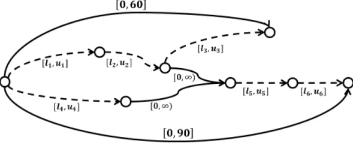
To generate a risk allocation, a certain form of the assump-tions on each duration must be established. For the subprob-lem to use STNU methods, the assumptions shall be in the form of variable [l, u] bounds. Figure 3 shows the space of possible risk allocations for the room setup example.
Given these variables, which have nonnegative domains, the risk allocation condition in Equation 1 for each chance
Figure 3: A parameterized STNU representing the space of risk allocations.
constraint may be expressed in terms of the durations’ cumu-lative density functions over these variables. Because prob-ability distributions are inherently nonlinear, this produces a nonlinear constraint program to solve. This is the program for the example:
Y i∈{1,2,3} (Fi(ui) − Fi(li)) ≥ 1 − 0.02 (2) Y i∈{1,2,4,5,6} (Fi(ui) − Fi(li)) ≥ 1 − 0.05. (3)
Equation 2, taking its form from Equation 1, expresses the risk allocation constraint for room A’s chance constraint. Indices 1, 2, and 3 are the durations in A’s relevant sub-plan. The expression under the product is the probability mass (1 − δi) covered by the risk allocation assumption on
a duration, and 0.02 is the chance constraint’s risk bound ∆. Equation 3 is an analogous constraint for room B’s risk allocation.
STNU controllability
A plausible STNU for the room setup example that satis-fies the constraint program is shown in Figure 4. There ex-ist efficient algorithms for checking STNU controllability, which also produce scheduling policies if the STNU is con-trollable (Vidal and Fargier 1999) (Morris and Muscettola 2000) (Morris and Muscettola 2005) (Stedl and Williams 2005) (Shah et al. 2007) (Nilsson, Kvarnstr¨om, and Doherty 2014). Thus, running one of these algorithms on the room setup STNU would produce a valid solution for the original chance-constrained problem. Because this paper is restricted to static policies, a strong controllability algorithm suffices.
In this room setup example, the STNU is indeed strongly controllable: In the worst case, room A would be prepared by time 21 + 19 + 16 = 56, which satisfies its one-hour requirement. Then, B might not be able to vacuum until time max{21 + 19, 40} = 40. But that is fine, because it would be prepared by time 40 + 35 + 14 = 89 with one minute to spare. Therefore, a valid static scheduling policy could assign the start of “vacuum B” any timepoint between 40 and 41.
Conflict discovery
If the STNU was not strongly controllable, then the subprob-lem needs to tell the master, so the master can generate an-other risk allocation. Fortunately, STNU controllability can
Figure 4: The resulting STNU after applying a risk alloca-tion. Dotted lines indicate uncontrollable durations; solid lines are simple temporal constraints.
yield a temporal conflict if it fails. The conflict is in the form of a negative cycle in the STNU. Thus, the cycle’s weight can be traced back to the risk allocation variables which con-tributed to it. The expression for the cycle’s weight in terms of those variables is then returned to the master, which adds it as a constraint in its constraint program, ensuring that the cycle remains non-negative in future iterations.
The solution process could work as follows on the exam-ple: First, the master would solve a constraint program con-sisting only of Equations 2 and 3. A feasible solution would be to assign 0 to all the lower bounds; 21, 19, 16 to the up-per bounds of room A’s three actions; and 45, 35, 15 to the upper bounds of room B’s actions. When checking the re-sulting STNU for strong controllability, one would discover that the combination of room B’s upper bounds exceeds its 90-minute constraint. Thus, the subproblem would return the temporal conflict u4+ u5+ u6> 90. In turn, the master
would invert the inequality and insert the condition into the constraint program. Then, the nonlinear solver may find that lowering u4to 40 would resolve the conflict while
preserv-ing B’s chance constraint. This new assignment would now pass the STNU check, so the static scheduling policy that would be output is to start “vacuum B” at time 40.
Note that there were no temporal constraints in the con-straint program on the first iteration. Instead, each succes-sive iteration adds a single temporal conflict to the program. Generally, some temporal constraints will be tighter than others, and hence more likely to be violated. Therefore, the conflict-directed approach tends to discover conflicts con-taining those constraints early on, which precludes the need to consider others before a controllable STNU is generated. The fact that only a few iterations may be needed, and that the program starts small and grows incrementally, is respon-sible for this approach’s efficient runtime performance.
Algorithm
The four key concepts and the running example from last section are formally expressed in an algorithm called Ru-bato. Rubato’s inputs and outputs are as specified in the Problem Statement section. This section explains Rubato line by line, and discusses its theoretical properties.
Throughout the solution process, Rubato maintains a con-straint list that serves as the master’s concon-straint program. There is no objective function in the problem statement, so a
Algorithm 1: Rubato
Input: a pSTN Np= hE , T i, where
T = hTr, Tc, Tpi.
Input: a set of chance constraints C over subsets of Tr.
Input: a mapping R : Tr7→ P (Tc∪ Tp) of relevant
durations for each temporal requirement. Output: a scheduling policy P for Np.
1 constraint list ← ∅; 2 foreach (∆i, Tir) ∈ C do
3 collect R(r) into Difor each r ∈ Tir; 4 product ←
Y
dj∈Di∩Tp
(Fj(uj) − Fj(lj)); 5 collect {product ≥ 1 − ∆i} into constraint list; 6 repeat
7 ok, risk allocation ← solve(constraint list); 8 if notok then return infeasible;
9 Nu← reformulate(Np,risk allocation); 10 ok, P , negative cycle ← checkSC(Nu); 11 ifok then return P ;
12 collect {negative cycle ≥ 0} into constraint list; 13 until timeout;
list of constraints suffices to represent the program. Lines 2 through 5 initialize the constraint list with all the nonlin-ear risk allocation constraints. Note that the constraint in line 5 matches the form given in Equation 1. The product in line 4 is taken over the relevant probabilistic durations for the ith chance constraint, hence the intersection of Di—all
the relevant actions’ durations—with the set of probabilistic durations Tp. The set Di is computed on line 3 by simply
collecting the relevant actions’ durations for all the temporal requirements that the ith chance constraint contains.
With the constraint list initialized, the main iterative loop of Rubato follows. The master begins, sending the constraint list through the nonlinear solver on line 7. The solver returns whether the list is a consistent, and a solution if so. The so-lution is an assignment to all [lj, uj] risk allocation bounds
on the probabilistic durations dj. If the solver did not find a
solution at this point, then Rubato returns on line 8 without a valid policy. Assuming the nonlinear solver is sound and complete, then this return statement is correct: If the solver could not even satisfy the chance constraints, then adding further constraints discovered by the subproblem will not help.
If a risk allocation was generated that respects the con-straint list so far, then Rubato passes it on to the subprob-lem. The pSTN is reformulated into an STNU on line 9, and then checked for strong controllability (SC) on line 10. Like the nonlinear solver, line 10 also performs a consis-tency check, but with an implicit set of constraints derived from the STNU. If it is consistent, i.e., the STNU is strongly controllable, then a scheduling policy P is produced. As discussed last section, although this policy works for the STNU, it works just as well for the pSTN under the risk bounds of the chance constraints, because the STNU is de-rived from the risk allocation. Thus, the policy may be
re-turned on line 11.
However, if the subproblem’s strong controllability check did not succeed, then it would have returned a negative cy-cle as the conflict. The negative cycy-cle would actually come from the distance graph representation of the STNU refor-mulated as an STN, according to the strong controllability algorithm. The cycle’s weight, however, can be expressed in terms of the STNU’s [lj, uj] bounds. Therefore, the
con-flict is that the cycle’s weight is negative, so to resolve it, the subproblem inserts the condition on line 12 that the cycle’s weight must be non-negative in future iterations of Rubato.
The master then starts the next iteration of Rubato, by solving the updated constraint list. This continues un-til either the constraint list becomes inconsistent, and Ru-bato returns infeasible, or the generated risk allocation pro-duces a strongly controllable STNU, and Rubato returns that STNU’s scheduling policy. These return conditions are sound by the reasoning above: If the constraint list is al-ready inconsistent, it cannot be made consistent again. If the STNU has a scheduling policy, then it must work for the pSTN as well.
Rubato is also complete with respect to risk allocation because the number of iterations is bounded. Specifically, there will not be more iterations than twice the number of temporal constraints |T |. To see this, consider if all the tem-poral constraints T were directly encoded into the constraint program from the start, as in the approach of (Fang, Yu, and Williams 2014). Each temporal constraint, whether a re-quirement or a duration, contributes two linear constraints to the constraint list, one for each of its lower and upper bounds. Thus, by the time 2|T | iterations have passed in Rubato, the constraint program will be just as constrained as in the non-conflict-directed case.
Suppose for the sake of contradiction that the iterations continue, where another risk allocation is generated, and a negative cycle is discovered. Then this negative cycle must yield the same condition as one discovered previously, be-cause algebraically the temporal network does not have any more unique constraints. However, if the condition was al-ready in the constraint list, then the solver could not have generated such a risk allocation in the first place. Therefore the iterations must end. In practice, if the pSTN is large and 2|T | iterations are too many to wait for, the loop may be truncated by a timeout.
Rubato’s completeness does hinge on the assumption that the nonlinear solver is itself sound and complete. The con-ditions under which this holds vary by solver. In our ex-periments described later, we used the Ipopt solver, which requires convex functions for completeness guarantees. For our chance-constrained scheduling problem, the discovered temporal conflicts are linear and hence convex, but the risk allocation constraints are expressed in terms of cumula-tive density distributions, which have no guarantee of being convex. Thus, any solution to the probabilistic scheduling problem–including prior art–faces the same issue. In prac-tice, probabilistic durations for most activities are modeled as a single-modal PDFs, whose cumulative distributions are convex.
Related Approaches
The presented approach has drawn from the major ideas of risk allocation and conflict-directed search. This section discusses these ideas in their original context and related scheduling work which has also leveraged these ideas.
To handle probabilistic dynamics within constraint sys-tems, a family of approaches use risk allocation to re-formulate the original stochastic problem into determinis-tic constraint optimization. Within the context of optimal chance-constrained path planning with obstacles, two ma-jor paradigms have been established. The first, convex risk allocation (CRA) allocates path planning decisions and risk allocation concurrently (Blackmore and Ono 2009), through a single convex optimization problem. The second, iterative risk allocation (IRA), analyzes the path for opportunities to redistribute the risk after each allocation (Ono and Williams 2008). Both solve the same optimization problem, but IRA follows its own rules in the path-planning context to improve the risk allocation, while CRA relies on generic optimization techniques.
The approach by (Fang, Yu, and Williams 2014) for chance-constrained scheduling falls in the vein of CRA. Their work had independently leveraged the first three ideas established in this work. Using a risk allocation that also maps the pSTN into an STNU, the strong controllability conditions are derived symbolically and directly encoded into the constraint program. These conditions are expressed as simple temporal constraints between the controllable events of the STNU. Therefore, the solver necessarily as-signs a grounded schedule to the events.
This work’s approach may be considered the IRA ana-logue of theirs. Rather than relying on the time-agnostic solver to improve the risk allocation, temporal conflicts are extracted and directly added to the constraint program. Note that these conflicts, being negative cycles, do not involve event variables, but only the risk allocation [l, u] bound vari-ables. Thus, the solver never generates a grounded schedule, but always an STNU, which leaves the flexibility to gener-ate a policy. Even a static policy is more flexible than a grounded schedule.
The idea of discovering conflicts and inserting them into the generator comes from conflict-directed search. Conflict-directed A* (CDA*) (Williams and Ragno 2007) is designed to solve discrete constraint programs efficiently by learning from past mistakes to reduce the search space. It begins like any other search, generating the search tree. When an as-signment is detected to be inconsistent with the program’s constraints, the reason and how to avoid it is recorded as a new rule for expanding the search tree. Thus, generating as-signments on the tree is the master problem, and learning conflicts is the role of the subproblem. CDA* was also ex-tended in the context of temporal planning (Yu and Williams 2013) (Yu, Fang, and Williams 2014) to offer continuous re-laxations to an STN’s constraints. Their STN temporal con-flicts are based on the same principle as the STNU concon-flicts described in this work.
Empirical Validation
Methods
This work is evaluated against two previous probabilistic approaches: the risk-minimization method by (Tsamardi-nos 2002), and the single-optimization chance-constrained method by (Fang, Yu, and Williams 2014). Benchmarks are run on each method over a range of problem sizes, and their runtime performances are compared. Although all three methods use risk allocation, the hypothesis is that this work’s conflict-directed approach would scale better than ei-ther previous approach: Neiei-ther of them discover conflicts along the way, so they must consider all temporal constraints in a single lump-sum optimization. Furthermore, the risk-minimization has to optimize a global risk metric, instead of just satisfying a set of chance constraints.
The authors of (Fang, Yu, and Williams 2014) kindly made available their collection of car-sharing scenarios as a common benchmark set. In these scenarios, a car-share company (e.g. Zipcar) manages a car fleet and allows drivers to book reservations on individual cars. A single car may be booked by multiple drivers in sequence. Each reservation consists of the driver visiting multiple city destinations. The driving time between destinations is probabilistic, according to local traffic conditions, but the amount of time one spends visiting each destination is controllable and bounded. All this activity is modeled as a pSTN. Each scenario may con-tain up to 20 cars, up to five reservations per car, and up to three destinations per driver.
The car-share needs all their vehicles back before the close of business that day. Therefore, they require a bound on the total time span of each car’s reservations, from its first to its last. A chance constraint is then placed over this requirement. All cars operations in parallel with the same time limit, and the chance constraint bound ∆ ranges from 10 percent to 40 percent.
The number of uncontrollable probabilistic durations in the pSTN, which is the total number of driving segments, is used to measure problem size. This is because each such duration adds two risk allocation variables, its lower and up-per bounds, to the optimization problem in all three meth-ods. Also, because each driver alternates between driving and visiting destinations, there is approximately one control-lable duration for each probabilistic one. Therefore, in the non-conflict-directed methods, the number of constraints in the optimization program is also proportional to the number of variables.
The algorithms are implemented in Common Lisp and linked to the Ipopt nonlinear optimizer (W¨achter and Biegler 2006), which is written in C++. Functionally, the imple-mentations for all three methods are quite similar: They all operate on the same pSTN input, and the risk expression in the chance-constrained methods is simply rewritten as the objective for risk-minimization.
Results
Figure 5 plots the runtime over problem size for each method running over the set of scenarios. The variation in runtime within each method is due to the inherent nondeterminism
in Ipopt’s execution: Indeed, the same scenario run on the same method multiple times yielded varying runtimes on the order shown in the graph. Despite the variation, each method exhibits a clear polynomial-like trend in runtime.
As predicted, the conflict-directed methods (diamonds) has the best performance. Whether looking at the average trend or the lower bound trend for each method, the new ap-proach runs approximately an order of magnitude faster than the other two methods (squares and triangles). This becomes evident as the problem size approaches 100 probabilistic du-rations, where the runtimes start reaching into the tens of seconds. A user would much prefer a solution method that computes within ten seconds than in two minutes.
Furthermore, prior art’s runtimes appear to grow slightly faster than the conflict-directed method does. This is be-cause while the number of risk allocation variables remains the same in all approaches, the conflict-directed method’s master problem collects only one additional conflict per it-eration. It turns out the conflicts are very informative: Out of more than 1500 scenarios, only 12 required up to four it-erations, 83 required three itit-erations, and the rest only one or two. Therefore, the master’s optimization problem actually grows slower than the size of the pSTN.
In addition, the overwhelming majority of the time for each iteration was spent in the solver as opposed to checking STNU controllability. Thus, the subproblem discovers con-flicts very efficiently, and the master’s optimization is still the bottleneck. This means the order-of-magnitude savings indicate primarily how much less work the master’s solver has to do, compared to prior art.
Finally, the risk-minimization method (triangles) demon-strates a slight but consistent edge over the single-optimization chance-constrained method (squares). The same trend was displayed in (Fang, Yu, and Williams 2014). This is interesting because the only difference is whether the risk expression is considered an objective or a chance con-straint. It appears that the solution methods employed by nonlinear solvers (Ipopt in this paper, Snopt in theirs) handle nonlinear objectives more efficiently than they do nonlinear constraints.
Conclusions
The main contribution of this work is to apply conflict-directed search to chance-constrained scheduling. The key insight is to decouple the reasoning about the temporal and chance constraints via a iterative master-and-subproblem so-lution method. The master generates risk allocations, refor-mulating the original pSTN into an STNU, which the sub-problem then checks for strong controllability.
Empirical results show that this work’s approach outper-forms prior art in probabilistic scheduling by nearly an order of magnitude. It is verified that much fewer constraints are considered, which significantly reduces the computational burden on the master nonlinear solver. The subproblem STNU checker incurs negligible runtime cost.
Figure 5: Runtime as a function of the number of uncontrollable durations in the car-sharing scenarios.
Acknowledgments
The authors thank David Wang and Erez Karpas for dis-cussing and reviewing the work, Eric Timmons and Enrique Fernandez for their code infrastructure and code support, and Cheng Fang and Peng Yu for making their Zipcar test cases available.
References
Blackmore, L., and Ono, M. 2009. Convex chance con-strained predictive control without sampling. In Proceedings of the AIAA Guidance, Navigation and Control Conference, 7–21.
Dechter, R.; Meiri, I.; and Pearl, J. 1991. Temporal con-straint networks. Artificial intelligence 49(1):61–95. Fang, C.; Yu, P.; and Williams, B. C. 2014. Chance-constrained probabilistic simple temporal problems. In Twenty-Eighth AAAI Conference on Artificial Intelligence. Gill, P. E.; Murray, W.; and Saunders, M. A. 2002. Snopt: An sqp algorithm for large-scale constrained optimization. SIAM journal on optimization12(4):979–1006.
Morris, P., and Muscettola, N. 2000. Execution of temporal plans with uncertainty. In AAAI/IAAI, 491–496.
Morris, P. H., and Muscettola, N. 2005. Temporal dynamic controllability revisited. In AAAI, 1193–1198.
Nieuwenhuis, R.; Oliveras, A.; and Tinelli, C. 2006. Solv-ing sat and sat modulo theories: From an abstract davis– putnam–logemann–loveland procedure to dpll (t). Journal of the ACM (JACM)53(6):937–977.
Nilsson, M.; Kvarnstr¨om, J.; and Doherty, P. 2014. Effi-cientidc: A faster incremental dynamic controllability algo-rithm. In Proceedings of the 24th International Conference on Automated Planning and Scheduling (ICAPS).
Ono, M., and Williams, B. C. 2008. Iterative risk allocation: A new approach to robust model predictive control with a joint chance constraint. In Decision and Control, 2008. CDC 2008. 47th IEEE Conference on, 3427–3432. IEEE.
Shah, J. A.; Stedl, J.; Williams, B. C.; and Robertson, P. 2007. A fast incremental algorithm for maintaining dis-patchability of partially controllable plans. In ICAPS, 296– 303.
Stedl, J., and Williams, B. C. 2005. A fast incremental dynamic controllability algorithm. In Proceedings of the ICAPS Workshop on Plan Execution: A Reality Check, 69– 75.
Tsamardinos, I. 2002. A probabilistic approach to robust execution of temporal plans with uncertainty. In Methods and Applications of Artificial Intelligence. Springer. 97–108. Vidal, T., and Fargier, H. 1999. Handling contingency in temporal constraint networks: from consistency to control-labilities. Journal of Experimental & Theoretical Artificial Intelligence11(1):23–45.
W¨achter, A., and Biegler, L. T. 2006. On the implementa-tion of an interior-point filter line-search algorithm for large-scale nonlinear programming. Mathematical programming 106(1):25–57.
Williams, B. C., and Ragno, R. J. 2007. Conflict-directed a* and its role in model-based embedded systems. Discrete Applied Mathematics155(12):1562–1595.
Yu, P., and Williams, B. 2013. Continuously relaxing over-constrained conditional temporal problems through general-ized conflict learning and resolution. In Proceedings of the Twenty-Third international joint conference on Artificial In-telligence, 2429–2436. AAAI Press.
Yu, P.; Fang, C.; and Williams, B. 2014. Resolving uncon-trollable conditional temporal problems using continuous re-laxations. In Twenty-Eighth AAAI Conference on Artificial Intelligence. AAAI Press.