Design optimization using soft computing techniques for extrusion blow molding processes

Publisher’s version / Version de l'éditeur:

Proceedings of 2002 NRC-NSC Canada-Taiwan Joint Workshop on Advanced

Manufacturing Technologies: 23-24 September 2002, London, Canada, pp. 73-84,

2002-09

READ THESE TERMS AND CONDITIONS CAREFULLY BEFORE USING THIS WEBSITE.

https://nrc-publications.canada.ca/eng/copyright

Vous avez des questions? Nous pouvons vous aider. Pour communiquer directement avec un auteur, consultez la

première page de la revue dans laquelle son article a été publié afin de trouver ses coordonnées. Si vous n’arrivez pas à les repérer, communiquez avec nous à PublicationsArchive-ArchivesPublications@nrc-cnrc.gc.ca.

Questions? Contact the NRC Publications Archive team at

PublicationsArchive-ArchivesPublications@nrc-cnrc.gc.ca. If you wish to email the authors directly, please see the first page of the publication for their contact information.

Archives des publications du CNRC

This publication could be one of several versions: author’s original, accepted manuscript or the publisher’s version. / La version de cette publication peut être l’une des suivantes : la version prépublication de l’auteur, la version acceptée du manuscrit ou la version de l’éditeur.

For the publisher’s version, please access the DOI link below./ Pour consulter la version de l’éditeur, utilisez le lien DOI ci-dessous.

https://doi.org/10.4224/23001683

Access and use of this website and the material on it are subject to the Terms and Conditions set forth at

Design optimization using soft computing techniques for extrusion

blow molding processes

Yu, Jyh-Cheng; Hung, Tsung-Ren; Juang, Jyh-Yeong; Thibault, Francis

https://publications-cnrc.canada.ca/fra/droits

L’accès à ce site Web et l’utilisation de son contenu sont assujettis aux conditions présentées dans le site LISEZ CES CONDITIONS ATTENTIVEMENT AVANT D’UTILISER CE SITE WEB.

NRC Publications Record / Notice d'Archives des publications de CNRC:

Design Optimization Using Soft Computing

Techniques For Extrusion Blow Molding Processes

Department of Mechanical Engineering National Taiwan University of Science and Technology

Taipei 106, Taiwan

Francis Thibault

Industrial Materials Institute Boucherville, Quebec, Canada

Abstract

The control of thickness distribution in extrusion blow molded parts is critical to assure product quality and reduce manufacturing cost. This study applies the soft computing strategy to determine the optimal die gap in the parison programming of extrusion blow molding process. Two types of optimization problem are addressed in this study. The process optimization objective is obtaining a uniform thickness of blown parts, and the design optimization objective is minimizing part weight subject to stress constraints. The finite element software, BlowView, is used to simulate the parison extrusion and the blow molding processes. However, the simulations are time consuming, and minimizing the number of simulation becomes an important issue. The proposed strategy, Fuzzy Neural-Taguchi and Genetic Algorithm (FUNTGA), first establishes a back propagation network using Taguchi's experimental array to predict the relationship between the design variables and the response. Genetic algorithm is then applied to search for the optimum design of parison programming. As the number of training samples is greatly reduced due to the use of orthogonal arrays, the prediction accuracy of the neural network model is closely related to the distance between sampling points and the evolved designs. The Reliability Distance is proposed and introduced to the Genetic Algorithm using fuzzy rules to modify the fitness function and thus improve search efficiency. The design of a HDPE bottle is used to illustrate the application of the process optimization, and the design of a gas tank is used to illustrate the application of performance. The design optimization uses ANSYS to find the stress distribution of blown parts under loads. The comparison of results using the optimization module of BlowView, Taguchi, and FUNTGA demonstrates the effectiveness of the proposed strategy.

Keywords:

1 Introduction

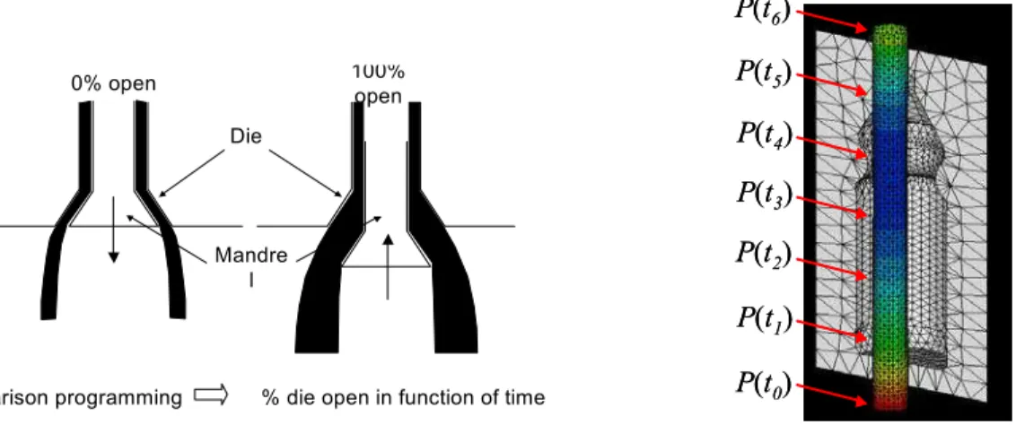
Extrusion blow molding is a low cost manufacturing process for complex hollow parts [1]. The process involves complex procedures such as parison extrusion, clamping, blow up, and cooling. First, the parison extrusion produces a molten thermoplastic tube coming out from the die. Once extrusion is finished, the parison is clamped and high-pressure air is blown into it to get the final part. To control the parison thickness over time, there is a mandrel that can move in and out to the die (Fig.1). Obviously, the parison thickness determines the thickness of the inflated part. The function of the parison programming is manipulating the die gap openings to obtain the desired thickness distribution of blown parts.

The programming points are specified by the extrusion time and the die gap opening of the parison. As the example part shown in Fig.2, we identify the die gap openings at 7 discrete extrusion times as the design variables:

P(t0), P(t1), P(t2), P(t3), P(t4), P(t5), and P(t6). These design variables will be adjusted to obtain the desired thickness distribution of blown parts. Two types of optimization problem are often encountered in the design of blow-molded parts by controlling the die gap programming. The process optimization objective is targeting a uniform part

thickness distribution of blown parts, and the design optimization objective is minimizing part weight subject to stress constraints. 0% open 100% open Die Mandre l

Parison programming % die open in function of time

Figure 1. The control of the parison thickness using the parison programming P(t₀) P(t₁) P(t2) P(t₄) P(t₃) P(t5) P(t6) P(t₀) P(t₁) P(t2) P(t₄) P(t₃) P(t5) P(t6)

Figure 2. Programming points of parison extrusion

Lee et al. [4] used a finite element model of thin film to simulate blow molding processes, and applied the feasible direction method to minimize the parison volume at the constraints of part thickness. Diraddo et al. [2] established a neural network to predict the distribution of parison thickness and applied Newton-Raphson method to obtain the final blow molded part specifications [3]. However, the investigation of the relationship between design variables and the wall thickness distribution of blown parts requires expensive experiments and time-consuming simulations. To reduce the number of experiments and simulations, an efficient strategy of data analysis is essential.

In this study, we apply an optimization strategy based on Taguchi’s experimental design [5] and soft computing techniques [6] to the optimization of parison programming to obtain the required thickness distribution. The proposed strategy establishes a local neural network based on Taguchi’s orthogonal array experiments and assumes the fuzzy inference to genetic algorithm to search for the optimal operating conditions. The finite element software, BlowSim [8], is used to simulate the parison extrusion and the blow molding processes.

The design of a gas tank targeting a uniform part thickness distribution illustrates the application of the proposed method to the process optimization. For the blown parts subjected to external and internal loading, an adequate part thickness profile has to be determined to satisfy the part mechanical performance. The aim is then to find the optimal die gap programming that will minimize the part weight and satisfy the part mechanical performance as well.

2 Optimization Strategy

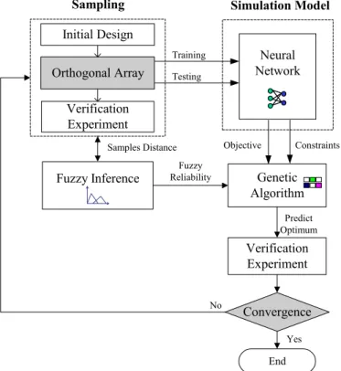
Taguchi’s method has proven its efficiency and simplicity in parameter design. The proposed optimization strategy, FUzzy Neural-Taguchi with Genetic Algorithm (FUNTGA) [10], applies Taguchi’s experimental design to the training and testing of a neural network model. The trained network becomes the function generator of the design fitness in the Genetic Algorithm. The optimum search using GA enhances the possibility for a better design than the conventional analysis of means (ANOM). A fuzzy inference of engineering knowledge is introduced to enhance the searching efficiency of GA. The flowchart of the optimization strategy is illustrated in Fig.3.

2.1 Taguchi’s Method

Inspired from statistical factorial experiments, Taguchi’s method features orthogonal arrays and analysis of mean (ANOM) to analyze the effects of design variables. Each variable is assumed to have finite levels (set points), such as two or three levels, within the investigating range. The orthogonal array is a type of fractional factorial experiments. The application of orthogonal arrays reduces the number of experiments, which is particular effective for design optimization involving expensive experiments or time-consuming simulations. For instance, instead of 27 experiments for three 3-level full factorial experiments, the L9 orthogonal array selects only nine treatments. ANOM study of experiment results reveals the effects of design parameters that are used to determine the optimal

level of each parameter. Knowing that Taguchi’s result is not a global optimum, however iterations of Taguchi’s method can provide a solution near to the optimum design.

Taguchi’s approach utilizes ANOM of fractional factorial experiments to predict the optimal design of the full factorial experiments. However, the prediction of the optimal design is sensitive to the selection of factorial levels and interaction effects. Also, the restriction of parameter values to factorial levels reduces the possibility of having better designs between preset levels.

Orthogonal Array Initial Design Verification Experiment Neural Network Training Testing Genetic Algorithm Objective Constraints

Sampling Simulation Model

Fuzzy Reliability Verification Experiment Predict Optimum Convergence No End Yes Fuzzy Inference Samples Distance

Figure 3 The Optimization flowchart of FUNTGA

(1,1,1) (3,3,3) (3,1,1) (3,3,1) (1,3,1) (1,3,3) (1,1,1) (3,2,1) (3,3,2) (2,1,2) (1,3,3) (1,2,2) (3,1,3) (2,2,3) (2,3,1)

(a) Full factorial exp. (b) Fractional factorial exp.

Figure 4 Full factorial and fractional factorial experiments for three variables

2.2 Neural-Taguchi network

Neural network technologies are effective in process control. The network is used to set up a simulation model for a complex nonlinear system. The back propagation network (BPN) is a type of supervised learning networks. Sampling data are divided into learning and testing samples. Learning samples are used to determine the weighting matrices, Wij and Wjo, among neurons and testing samples to determine the accuracy and the generality of the network.

Training samples are essential to the prediction quality of network models. This study employs Taguchi’s experimental design to select training samples to reduce the number of experiments and to maintain a good sample representation [7][9]. The steepest gradient method is assumed to train the weighting matrices. The verification experiment of the optimal design from the ANOM study will serve as a testing sample. The trained network can accurately predict responses for the parameter designs between factorial levels. Significant interactions often introduce complexity to experimental design and lead to erroneous prediction of optimal factorial levels. The network model can resolve interaction effects among variables. These features enable the network to explore a better design as compared with Taguchi’s additive model [5].

2.3 The search for the optimum of the Neural-Taguchi network

The trained Neural-Taguchi network can predict responses for the parameter combinations in the investigating range. Generic Algorithm is thus applied to search for the optimum. If the verification result of the predicted optimum is not satisfactory, the design will be used as an initial design and another set of orthogonal array experiments will be conducted. The results will be served as additional testing data for the network. The iteration process stops when the predicted optimum obtained from GA and the network converges.

The Neural-Taguchi network replaces Taguchi’s additive model to predict design outputs. The search for the optimum in the investigating range using GA will explore the possibility of better designs other than factorial points. However, the application of orthogonal arrays significantly reduces the number of training samples as compared with conventional random sampling. Owing to that better prediction accuracy will exist around sampling points, our approach introduces a fuzzy inference to steer the search direction of GA.

2.3.1 Normalization of design parameters

To facilitate the calculation of the distance among designs, the values of the set points of continuous variable xk are normalized to zk using the following transformation

(

)

(

)

where max(xk) represents the maximum and min(xk) represents the minimum values of the factorial variable xk. Thus the normalized factorial values of an equal spaced three-level continuous variable, x1, will become (z11, z12, z13) = (-1, 0, 1). For discrete variables, the factorial values are equally assigned between -1 and +1.

2.3.2 The Reliability Distance

The mean Euclid distances between predictive designs, Di, and the sample data Sj are defined as follows

(

)

∑

where n represents the number of variables.

Since predictions around the sampling points of the trained network will have higher accuracy, we proposed to use the Reliability Distance of a predictive design as the minimum factorial distance between the prediction and

sampling data. ) min(ij

i r

RD = (3)

Smaller RD results in higher prediction accuracy. Also, the distance of an interpolating design is assumed

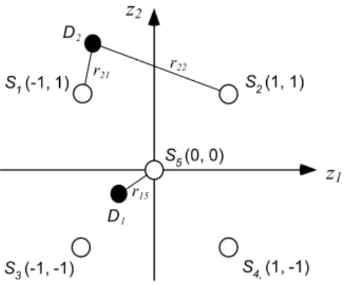
negative and the distance of an extrapolating design is assumed positive. For instance, the Reliability Distance of D1 in Fig.5 is negative and the Reliability Distance of D2 is positive.

r15 z1 z2 r21 r22 S_4, (1, -1) S₅ (0, 0) S₁ (-1, 1) S₂ (1, 1) S₃ (-1, -1) D1 D2

Figure 5 The factorial distances of predicted designs

2.3.3 The fuzzy rules of prediction accuracy

The Reliability Distance of a predictive design determines the Prediction Reliability (PR) of the design. The

reliability of the predicted design decreases when the absolute value of RD increases. Also, the reliability of

extrapolating designs is often much worse than the interpolating designs. Based on the above characteristics of neural network, we propose to use fuzzy rules of the design reliability as follows

R1: If RD is PB then prediction reliability is Bad

R2: If RD is PM then prediction reliability is Poor

R3: If RD is PS then prediction reliability is Fair

R4: If RD is ZE then prediction reliability is Excellent

R5: If RD is NS then prediction reliability is Good

R6: If RD is NM then prediction reliability is Fair

R7: If RD is NB then prediction reliability is Poor

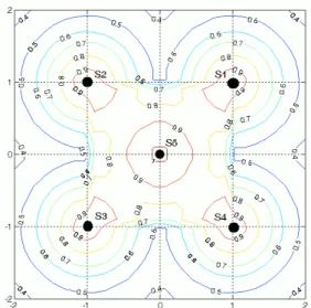
Seven levels are defined to describe the condition variables: PB(Positive Big), PM(Positive Medium), PS(Positive Small), ZE(Zero), NS(Negative Small), Negative Medium (NM), and NB(Negative Big). Five levels are defined to describe the assessment results: Excellent, Good, Fair, Poor, and Bad. Standard membership functions associated with these statements are illustrated in Fig.6 and Fig.7. Fig.8 is the reliability contour plot for the two dimensional case using the fuzzy inference. The solid dots represent the training samples.

PS PM PB NB NM NS Interpolation Extrapolation 0 ZE 1.0 RD 0.5 1.0 1.5 -0.5 -1.0 -1.5

Figure 6 Membership functions of condition variables

Reliability 1.0 0.8 0.6 0.1 0.35 Excellent Good Fair Poor Bad μ 1.0

Figure 7 Membership functions of assessment variables

2.3.4 Genetic Algorithm

FUNTGA uses the Genetic Algorithm to search the optimum of the Neural-Taguchi network. However, the accuracy of the network is limited due to the reduced number of training samples. The design fitness obtained from the network is thus modified to reflect the characteristics of prediction accuracy. The search of the local optimum will then be restricted to the surroundings of the training samples to prevent the possible erroneous prediction.

   < > × = 0 Fitness if , / 0 Fitness if , net net PR Fitness PR Fitness Fitness net net GA (4)

Figure 8 Reliability contour plot for two variables

3 Optimization of Blow Molding Parameters for Process Design

This work uses the proposed optimization strategy to get the optimal parameter design of extrusion blow molding process for the gas tank case of the Kautex Textron Company. The gas tank is made of High Density Polyethylene (HDPE). The design objective is to target a uniform part thickness of 5 mm. The blow molded part

thickness distribution is estimated by using the BlowSim software. Fig.9 shows that the die gap openings at 13 discrete extrusion times are selected as the control variables: P(t1), P(t2),…P(t12), and P(t13).

Figure 9 The control points of the gas tank example

3.1 The Objective Function

A quality blow molding part requires on-target and uniformly distributed part thickness. To reach this goal, we propose to define an objective function as the average quality loss due to the deviation of thickness,

(

)

∑

where ti stands for the thickness of node i, T for the target thickness, and n for the total number of nodes of the

simulation model.

Any deviation from the target thickness will cause quality loss. The average quality loss can be divided into two parts: the mean deviation from the target thickness and the thickness variation around mean as the following

(

)

(

)

∑

∑

where t is the mean stress and s2 is the sampling variance. Reducing the quality loss leads to a thickness

distribution of a smaller variance and a mean thickness closer to the target.

3.2 Taguchi’s parameter design

3.2.1 Experimental Design

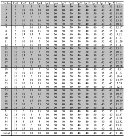
The die gap openings at 13 discrete extrusion times are selected as the control factors. The design optimization manipulates the die gap openings of programming points to obtain a uniform thickness distribution. The initial design adopts a uniform die gap opening of 10% for first four control points and 20% for the rest. The L36 orthogonal array is selected as the experimental design (Table 1). For each opening, we assume a three-levels variation around the initial design located in the middle of the design space. The range between upper and lower levels represents the design space.

Table 1. L36 orthogonal array

L36 Run Ppt1 Ppt2 Ppt3 Ppt4 Ppt5 Ppt6 Ppt7 Ppt8 Ppt9 Ppt10 Ppt11 Ppt12 Ppt13 Loss. 1 5 5 5 5 30 30 30 30 30 30 30 35 35 4.93 2 5 10 10 10 40 40 40 40 40 40 40 40 40 10.61 3 5 15 15 15 50 50 50 50 50 50 50 45 45 18.48 4 5 5 5 5 30 40 40 40 40 50 50 45 45 13.85 5 5 10 10 10 40 50 50 50 50 30 30 35 35 13.14 6 5 15 15 15 50 30 30 30 30 40 40 40 40 10.17 7 5 5 10 15 30 40 50 50 30 40 40 45 40 12.07 8 5 10 10 15 30 40 50 30 30 40 50 45 35 11.78 9 5 15 15 5 40 50 30 40 40 50 30 35 40 9.62 10 5 5 5 15 40 30 50 40 50 40 30 45 40 11.53 11 5 10 10 5 50 40 30 50 30 50 40 35 45 11.29 12 5 15 15 10 30 50 40 30 40 30 50 40 35 11.47 13 10 5 10 15 30 50 40 30 50 50 40 35 40 13.01 14 10 10 15 5 40 30 50 40 30 30 50 40 45 10.91 15 10 15 5 10 50 40 30 50 40 40 30 45 35 12.63 16 10 5 10 15 40 30 30 50 40 50 50 40 35 13.19 17 10 10 15 5 50 40 40 30 50 30 30 45 40 12.08 18 10 15 5 10 30 50 50 40 30 40 40 35 45 10.76 19 10 5 10 5 50 50 50 30 40 40 30 40 45 15 20 10 10 15 10 30 30 30 40 50 50 40 45 35 11.63 21 10 15 5 15 40 40 40 50 30 30 50 35 40 10.4 22 10 5 10 10 50 50 30 40 30 30 50 45 40 14.89 23 10 10 15 15 30 30 40 50 40 40 30 35 45 7.59 24 10 15 5 5 40 40 50 30 50 50 40 40 35 12.4 25 15 5 15 10 30 40 50 50 30 50 30 40 40 10.65 26 15 10 5 15 40 50 30 30 40 30 40 45 45 10.34 27 15 15 10 5 50 30 40 40 50 40 50 35 35 12.6 28 15 5 15 10 40 40 30 30 50 40 50 35 45 10.69 29 15 10 5 15 50 50 40 40 30 50 30 40 35 15.62 30 15 15 10 5 30 30 50 50 40 30 40 45 40 11.44 31 15 5 15 15 50 40 50 40 40 30 40 35 35 11.22 32 15 10 5 5 30 50 30 50 50 40 50 40 40 18.57 33 15 15 10 10 40 30 40 30 30 50 30 45 45 8.08 34 15 5 15 5 40 50 40 50 30 40 40 40 45 12.32 35 15 10 5 10 50 30 50 30 40 50 50 35 40 13.11 36 15 15 10 15 30 40 30 40 50 30 30 40 45 8.63 Initial 10 10 10 10 40 40 40 40 40 40 40 40 40 11.48 3.2.2 Parameter design

Taguchi’s method applies the analysis of means (ANOM) to estimate parameter sensitivities. Fig.10 represents the factor effects for each die opening on objective. The additive model estimates the optimum treatment combination to be A1B3C3D2E2F1G1H1I1J1K1L1M3. The BlowSim simulation of Taguchi’s optimum shows the loss of 6.44, which is not the best design in Table 1. The failure of Taguchi’s approach might due to interactions among design variables and strong system non-linearity.

Figure 10 Factor effects plot of control variables

3.3 Design optimization using FUNTGA

3.3.1 The establishment of the neural network

FUNTGA provides a more efficient and accurate optimum search using the same experimental data of Taguchi’s experiments. The L36 orthogonal experiments are divided into two smaller orthogonal arrays as differentiated by the shade in Table 1. 18 experiments are used as training samples and the other 18 experiments are used as testing samples. There are 15 neurons in the hidden layer. The initial learning rate is set to 1.0 and the initial momentum term is set to 0.5.

3.3.2 Optimum search using GA

The fuzzy rules for prediction accuracy are applied to GA to improve the searching efficiency. The fitness function is defined as follows,

PR loss Avg

FitnessGA =− _ / (7)

The trained network will then be used as the function generator for each chromosome combination. The parameters of Genetic Algorithm used in this study are listed in Table 2.

Table 2 Genetic Algorithm parameters

Population size

Pool selection style Scale style Cross Over rate

Mutation rate Max iteration

37 Parent and offspring Linear scale 0.75 0.1 100

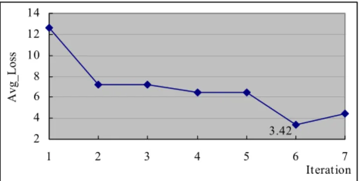
The search result of GA will then be added to the training samples of the neural model to further improve the network accuracy. The optimization process iterates until the results converge. The iteration history of FUNTGA is shown in Fig.11. 3.42 2 4 6 8 10 12 14 1 2 3 4 5 6 7 Iteration Avg_Loss

3.4 Comparison of results

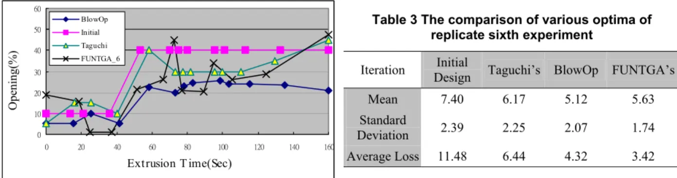
Fig.12 and Table 3 present the die gap openings of the parison programming and the optimization results obtained from Taguchi’s method, BlowOp, and FUNTGA. BlowOp is a BlowSim optimization module that uses a gradient-based algorithm to control the die gap openings of the parison programming points. Although BlowOp optimum provides a mean thickness closer to the target of 5 mm, FUNTGA’s optimum exhibits a more uniform distribution and the lowest quality loss.

8 Extrusion T ime(Sec) Opening(%) BlowOp Initial Taguchi FUNTGA_6

Figure 12 The optimal designs from various methods

Table 3 The comparison of various optima of replicate sixth experiment

Iteration Initial

Design Taguchi’s BlowOp FUNTGA’s

Mean 7.40 6.17 5.12 5.63

Standard

Deviation 2.39 2.25 2.07 1.74

Average Loss 11.48 6.44 4.32 3.42

4 Optimization of Blow Molding Parameters for Performance Design

This work applies the proposed optimization strategy to get the optimal parameter design of extrusion blow molding process for the HDPE bottle of the Lear Corporation. Two types of loading will be investigated: an internal pressurization at 110 (psi) and a top displacement of 5 (mm) during 5 seconds as illustrated in Fig.13. The maximum allowable stress, corresponding to the ultimate tensile strength of the material, is set to 33 MPa. For this material, the Young’s modulus is 879 MPa and we assume that the thickness part shrinkage is 3%. From a part thickness distribution obtained from BlowSim, ANSYS software is used to make the structural analysis for the specified loading [11].

P T

Figure 13 The mechanical loading of the HDPE bottle: the internal pressurization and the top displacement

σ

Figure 14 The illustration of the design objective for performance optimization

4.1 The Objective Function

The initial formulation for this optimization can be represented as follows,

Minimize: Part_Weight[P(tj)]

Design Variable: P(tj)

Where P(tj) are the gap openings of the controlling points, si are the stresses of node i, σa is the allowable stress of the material, P is the internal pressure, and T is the top displacement.

The objective function is modified to obtain a wall thickness distribution of minimal weight subject to stress constraints. The reduction of an element thickness results in the increase of its stress level. Consequently, the design objective can be replaced by a minimization of the stress variance around the stress mean close to the stress constraint. The smaller variance of the stress distribution, the closer the mean can be moved to the allowable material strength, that leads to thinner elements, and thus minimal part weight. However, any element stress exceeding the allowable strength might result in part failure. In this work the constrained optimization is replaced by an unconstrained minimization of the variance of stress distribution around the allowable stress level using the external penalty method as illustrated in Fig.14.

The objective function (Eq. [8]) contains two portions: the quality loss due to variation of stress distribution and the penalty loss due to constraint violation

(

)

∑

∑

where n is the total number of nodes of the simulation model.

The quality loss due to variation of stress distribution is estimated by the mean squared deviation of the element stress from the allowable stress level that is similar to the objective used in the previous process optimization. The average quality loss can be divided into two parts: the deviation of the mean stress from the allowable strength and the variation of the stress around mean.

The second portion of the modified objective function, the penalty loss, is estimated using a second order singularity function. This portion accounts for the penalty of elements violating the stress constraint.

   > − ≤ = > − < a i a i a i a i s s s s σ σ σ σ if , ) ( if , 0 2 2 ₍₉₎

The search for the design of minimum objective function will provide a thickness of minimum part weight while satisfying the stress requirement.

4.2 Taguchi’s parameter design

4.2.1 Experimental Design

The die gap openings at 7 discrete extrusion times are selected as the control factors: Pi(t0), Pi(t1), Pi(t2), Pi(t3),

Pi(t4), Pi(t5), and Pi(t6). The initial design adopts a uniform die gap opening of 75%. The L18 orthogonal array is selected as the experimental design. For each opening, we assume a three-levels variation around the initial design located in the middle of the design space. The range between upper and lower levels represents the design space. We assume 40% variation range.

) log( 10 _ /N ratio MOBJ S =− × (10) 4.2.2 Parameter design

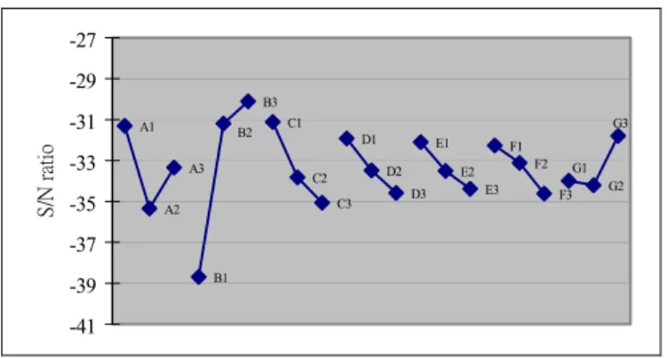
Taguchi’s method applies the analysis of means (ANOM) to estimate parameter sensitivities. Fig.15 represents the factor effects for each die opening on the S/N ratio. A design with higher S/N ratio has a smaller value of the objective function. Taguchi’s additive model estimates the optimum treatment combination to be A1B3C1D1E1F1G3. The BlowSim simulation result of Taguchi’s optimum shows a S/N ratio of –27.45 that is worse than the S/N of the initial design of –25.6. The failure of Taguchi’s approach might due to interactions among design variables and strong system non-linearity.

A1 A2 A3 B1 B3 C1 C2 C3 D1 D2 D3 E1 E2 E3 F1 F2 F3 G2 B2 G1 G3 -41 -39 -37 -35 -33 -31 -29 -27

Figure 15 The factor effects plot of the bottle case

4.3 Design optimization using FUNTGA

4.3.1 Establishment of neural network

FUNTGA uses L18 orthogonal experiments as learning samples for the Back Propagation Network (BPN) of the extrusion blow molding process. The initial design and Taguchi’s optimum design are used as testing samples for the trained network. There are 14 neurons in the first hidden layer and 6 neurons in the second hidden layer. The initial learning rate is set to 1.4 and the initial momentum term is set to 0.5. The RMS error reduces to 0.055 after 16000 epochs.

4.3.2 Optimum search using GA

The fuzzy rules for prediction accuracy are applied to GA to improve the searching efficiency. The fitness function is defined as follows,

PR ratio N S

FitnessGA=( / _ )/ (11)

The trained network will then be used as the function generator for each chromosome combination. The parameters of Genetic Algorithm used in this study are listed in Table 4.

Table 4 Genetic Algorithm parameters

Population size Pool selection style Scale style Cross Over rate Mutation rate Max iteration 20 Parent and offspring Linear scale 0.8 0.01 300

4.4 Comparison of the results

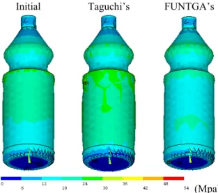
Fig.16 shows the profiles of optimal die gap openings of parison programming and Table 5 compares the stress distributions of the initial design and the optimal one obtained from Taguchi’s method and FUNTGA strategy. Taguchi’s ANOM approach is disturbed by parameter interactions and system non-linearity. Taguchi’s optimum provides a mean stress closer to the allowable strength 33 MPa. However, the large variance of the stress distribution results in stronger violation of stress constraints than the initial design. FUNTGA’s optimum exhibits a mean thickness close to the allowable and the smallest deviation in three designs, which leads to a design of smaller weight while satisfying the stress constraints. Fig.17 presents the stress distributions of three designs.

5 Conclusions

This study presents how to apply soft computing technology to determine the optimum die gap openings of parison programming of extrusion blow molding process. Taguchi’s method is cost effective to obtain an improved design in a few experiments. However, possible interactions among parameters and system non-linearity could complicate parameter design. Instead of using ANOM of Taguchi’s experimental design, FUNTGA establishes a back propagation network using Taguchi’s experimental data. Heuristic knowledge of prediction accuracy is

applied to GA using fuzzy rules to steer the search direction. The proposed strategy works well with both the process optimization and the performance optimization examples. Extra iterations using FUNTGA’s approach are possible if further improvement is desired. The comparison of results demonstrates the effectiveness of the proposed strategy. 0 20 40 60 80 100 0 10 20 30

Extrusion T ime (Sec)

Open (%

)

Initial Taguchi's FUNTGA's

Figure 16 The optimal designs from various methods

Initial Taguchi’s FUNTGA’s

(Mpa)

Figure 17 The comparison of the stress distribution Table 5 The comparison of various optima

Mean Stress

Std.Dev.

Stress Quality Loss

Penalty Loss Objective Function Initial 15.9 6.4 335.1 33.7 368. 8 Taguchi’s 16.6 7.3 322.4 233.2 555.6 FUNTGA’s 16.0 6.1 324.9 2.3 327.2

Acknowledgments

The authors would like to thank the National Science Council of the Republic of China for financially supporting this research under Contract No. NSC90-2212-E-011-022.

References

[1]. D. Rosato and D. Rosato, Blow Molding Handbook, Hanser Publisher, Munich, 1989.

[2]. R. W. Diraddo and A. Garcia-Rejon, “On-Line Prediction of Final Part Dimensions in Blow Molding: A Neural Network Computing Approach”, Polymer Engineering and Science, MID-JUNE, v33, n11 (1993) 653-664,.

[3]. R. W. Diraddo and A. Garcia-Rejon, “Profile Optimization for The Prediction of Initial Parison Dimensions From Final Blow Moulded Part Specifications”, Computers Chem. Engng, v17 n8 (1993) 751-764.

[4]. D. K. Lee and S. K. Soh, "Prediction of Optimal Preform Thickness Distribution in Blow Molding", Polymer engineering

and science, v36 n11 (1996).

[5]. G. Taguchi, “Performance Analysis Design.” Int. Journal of Production Research, 16 (1978) 521-530.

[6]. J. S. Jang, C. T. Sun and E. Mizutani, Neuro-Fuzzy and Soft Computing: a computational approach to learning and

machine intelligence, Prentice-Hall, (1997).

[7]. C. T. Su, C. C. Chiu and H. H. C, “Parameter Design Optimization via Neural Network And Genetic Algorithm”, Int.

Journal Of Industrial Engineering, 7(3) (2000) 224-231

[8]. BlowSim, 6.0, Industrial Materials Institute, National Research Council Canada 1999.

[9]. G. J. Wang, J. C. Tsai, P. C. Tseng and T. C. Chen, “Neural-Taguchi Method for Robust Design Analysis”, Journal of the

Chinese Society of Mech. Eng., v19 n2 (1998) 223-230

[10]. J. Yu, X. Chen, and T.R. Hung (2001) Optimization of Extrusion Blow Molding Using Soft Computing and Taguchi Method , Proceedings of the Sixth International Conference on Computer Supported Cooperative Work in Design, July 12-15, 2001, London, Ontario, Canada.

[11]. J. Yu, T.R Hung, and F. Thibault (2002) “Performance Optimization of Extrusion Blow Molded Parts Using Fuzzy Neural-Taguchi Method and Genetic Algorithm”, ASME Design Automation Conference 2002, Sept., 2002, Montreal, Canada.