Colour image filtering with component-graphs

HAL Id: hal-01695069

https://hal.univ-reims.fr/hal-01695069

Submitted on 15 Feb 2018

HAL is a multi-disciplinary open access

archive for the deposit and dissemination of

sci-entific research documents, whether they are

pub-lished or not. The documents may come from

teaching and research institutions in France or

abroad, or from public or private research centers.

L’archive ouverte pluridisciplinaire HAL, est

destinée au dépôt et à la diffusion de documents

scientifiques de niveau recherche, publiés ou non,

émanant des établissements d’enseignement et de

recherche français ou étrangers, des laboratoires

publics ou privés.

Colour image filtering with component-graphs

Benoît Naegel, Nicolas Passat

To cite this version:

Benoît Naegel, Nicolas Passat.

Colour image filtering with component-graphs.

Interna-tional Conference on Pattern Recognition (ICPR), 2014, Stockholm, Sweden.

pp.1621-1626,

Colour image filtering with component-graphs

Benoît Naegel

Nicolas Passat

Université de Reims Champagne-Ardenne CReSTIC

Reims, France

Abstract—Mathematical morphology, initially devoted to

bi-nary and grey-level image processing, also offers opportunities to develop efficient tools for multivalued – and in particular, colour – images. In this context, connected operators are increasingly considered as a relevant way to obtain such tools, mainly for image filtering and segmentation purposes. In this article, we focus on connected operators based on component-trees and their extension to multivalued images, namely component-graphs. Beyond the classical colour-handling strategies, we show how component-graphs can be algorithmically used to efficiently handle the whole structural information gathered by colour spaces, in order to finally design original image filtering tools.

I. INTRODUCTION

Mathematical morphology [1] was first defined on binary images, and then on grey-level ones [2]. Its extension to multivalued (e.g., colour, multispectral, label) images is an important task, motivated by potential applications in multiple areas. Several contributions have been devoted to this specific purpose (see [3] for a recent survey).

In the theoretical framework of mathematical morphology, the notion of connected operators [4], [5] gathers powerful image processing tools that mainly rely on hierarchical image representations, i.e., tree structures, which are indeed partition hierarchies: component-trees [6], level-line trees [7], binary partition trees [8], etc. The extension of the induced tree-based connected operators to multivalued images is an increasingly considered research field.

The difficulties raised by these extensions depend on the impact of the “colour” space on the induced data structures. A first family of strategies consists of preserving the tree structure, as proposed in [9] for binary partition trees, in [10] for level-line trees, or in [11] for component-trees. A second consists of dealing with more complex data structures that are no longer trees, but directed acyclic graphs (DAGs), as proposed for component-tree extensions. Such DAG-based approaches – studied in multivalued imaging, but also in non-standard connectivity approaches [12], [13] – are more challenging. However, they allow us to use the full structural information gathered by the colour spaces, and thus to develop accurate image processing tools.

We focus on the case of the component-tree and its exten-sions. In order to handle – partially ordered – colour spaces, the component-tree – that requires a total order on the value spaces

The research leading to these results has received funding from the French

Agence Nationale de la Recherche (Grant Agreement ANR-10-BLAN-0205).

– generally relies on two strategies, namely marginal and vec-torial processing [14]. The first consists of splitting the value set into several totally ordered ones, while the second defines ad hoc total order relations on them. However, both strategies alter the structural information gathered by the colour spaces. To tackle this issue, a multivalued extension of the component-tree, namely the component-graph, was introduced in [15], and declined under several variants of DAGs, of varying space complexity and richness [16].

In this article, we first recall the basics of component-graphs (Sec. II). Then, we propose algorithmic solutions to build the different variants of component-graphs, and to recon-struct the associated filtered images, with a focus on colour spaces, that are organised as lattices (Sec. III). We finally propose experimental results of filtering on colour images, in the standard RGB and HSV spaces (Sec. IV).

II. COMPONENT-GRAPH

Let Ω be a nonempty finite set. Given an adjacency relation on Ω, we define for any X ⊆ Ω, the (equivalence) connectedness relation as the reflexive-transitive closure of this adjacency on X. The set of all the connected components (i.e., equivalence classes) of X, is noted C[X].

Let V be a nonempty finite set equipped with an order relation 6. We note < and ≺ the strict and cover relations associated to 6, respectively. We assume that (V, 6) admits a minimum, noted ⊥.

Let us consider an image I : Ω → V. Each binary level set λv(I) = {x ∈ Ω | v 6 I(x)} ⊆ Ω is divided into connected

components, gathered into the partition C[λv(I)]. The union

Φ =[

v∈V

C[λv(I)] (1)

of all these partitions can be equipped with the inclusion ⊆. Let us suppose that (V, 6) is totally ordered, i.e., I is a grey-level image. We can then define the component-tree of I.

Definition 1 ([6]): The component-tree T of I is the Hasse

diagram of the partially ordered set (Φ, ⊆).

Less formally, the component-tree is a hierarchical data structure – i.e., a rooted tree – that models a grey-level image by considering its binary level sets obtained from successive thresholdings. Its root is Ω, while its leaves are the flat zones of I of locally maximal values.

The component-tree can be efficiently built [17]. Moreover, it is well-suited for grey-level image filtering methods relying

(a) I : Ω → V a d b c e f g h j i (b) (V, ≺) A (c) λa(I) B F (d) λb(I) D E C (e) λc(I) G M (f) λd(I) H N (g) λe(I) I O X X (h) λf(I) J K (i) λg(I) Q L (j) λh(I) R X X (k) λi(I) P S (l) λj(I) A G H C B D E F S Q R I J K M N O L P (m) G A C B S R I J K L P (n) ˙G A B S R I K L P (o) ¨G

Fig. 1. (a) An image I : Ω → V, with V = {a, . . . , j}. (b) The Hasse diagram of the ordered set (V, 6) (each value of V is associated to a “false” colour). (c–l) Thresholded images λv(I) for v ∈ V. (m–o) The component-graphs of I.

The letters (A–S) in nodes correspond to the connected components in (c–l).

on attribute-based [18] strategies. In particular, component-trees have been involved in a classical antiextensive filtering scheme [6], [19] which will be recalled in Sec. III.

If we relax the totality constraint on 6, then T does no longer have a tree structure, in most cases. This has motivated the introduction of a more general notion of component-graph. To define this notion, we enrich the set Φ, by assigning to each connected component the value of its level set. The obtained set of valued connected components is then defined as

Θ =[

v∈V

C[λv(I)] × {v} (2)

We then extend the inclusion relation on Φ by considering these values. We obtain the order relation E on Θ defined as

(X1,v1) E (X2,v2) ⇔ (X1⊂ X2) ∨ ((X1=X2) ∧ (v26v1)) (3)

We can finally define the notion of component-graph as follows.

Definition 2 ([15], [16]): The component-graph G of I is

the Hasse diagram (Θ, ◭) of the partially ordered set (Θ, E). The component-graph can be declined into three variants (see Fig. 1), noted G, ˙G and ¨G – of decreasing space complexity and richness – by also considering the following two subsets of Θ, namely

˙

Θ =_{{(X, v) ∈ Θ | ∀(X, v}′_{) ∈ Θ, v ≮ v}′} (4) ¨

Θ =_{{(X, v) ∈ Θ | ∃x ∈ X, v = I(x)} (5)}

By contrast with the component-tree, the component-graph does not have a tree structure, in general. Nevertheless, it is a relevant extension of the component-tree since both notions are compatible for grey-level images.

Proposition 3 ([16]): If (V, 6) is a totally ordered set, then

two of the three variants of component-graphs, namely ˙G and ¨

G, are isomorphic to the component-tree. III. FILTERING METHODOLOGY

Component-graphs inherit the (de)composition formula classically associated to component-trees, namely

I = ≤

_

K∈Θ

CK (6)

whereWis the supremum operator, ≤ is the pointwise order on functions induced by 6, and for any (X, v) ∈ Θ, C(X,v): Ω → V is the cylinder function defined by C(X,v)(x) = v if x ∈ X and

⊥ otherwise.

In the framework of component-trees, this formula led to an antiextensive filtering scheme for grey-level images [6], [19]. This scheme can then be extended to the case of component-graphs. It consists of the following three successive steps:

(i) construction of the component-graph G of I; (ii) reduction of G into a reduced component-graph bG; (iii) reconstruction of a filtered image bI ≤ I from bG.

In [20], Step (ii) was already discussed. In the sequel of this section, we mainly describe how to deal with Step (i), i.e., how to build the component-graph(s); and how to deal with Step (iii), with a focus on the colour (lattice) spaces.

A. Component-graph construction

By contrast with the component-tree, computing a component-graph raises structural and algorithmic difficulties. In particular, the classical component-tree construction algo-rithms [17] cannot be directly extended to the cases where (V, 6) is not totally ordered. More precisely, two main issues have to be faced: (i) the existence of neighbour points with non-comparable values, that requires to potentially explore, around each point, an extensive area to define the links between nodes; and (ii) the maintenance of the transitive reduction of the graph. In this context, we present algorithms for the computation of G, ˙G and ¨G.

Algorithm 1: Computation of G (or ˙G)

Input: I : Ω → V (input image) Input: (V, 6) (lattice of values) Output: Component-graph G (or ˙G)

1 foreach v ∈ V do 2 foreach p ∈ Ω do 3 foreach q ∈ Ω do 4 inQueue[q]=false 5 if isLeq(v,I(p)) then 6 fifo.push(p) 7 inQueue[p]=true

// Create new node

8 n=makeNode(v) 9 graph.insert(n)

10 while (!fifo.empty()) do 11 q=fifo.front()

// Add pixel q to current node n

12 n.add(q) 13 foreach neighbour r of q do 14 if isLeq(v,I(r)) then 15 if inQueue[r]==false then 16 fifo.push(r) 17 inQueue[r]=true 18 foreach n ∈ graph do

19 foreach m ∈ graph with m ,n do 20 if m.area ≤ n.area then

21 if isIncluded(m,n) ∧ isLeq(n.value,m.value) then 22 n.addChild(m)

23 graph=computeTransitiveReduction(graph)

// For the G˙ component-graph only

24 graph=keepMaximalElements(graph)

1) Data structures: Each node of the graph is stored in

a structure node. As ◭ denotes a father-child relationship, each node has to store its direct fathers and direct children, respectively, in two arraysfathersandchildren. A node also contains its original valuevalue, its current value in the filtered image curValue, a Boolean active indicating if it is currently preserved or discarded, and a set of attributes

(area, contrast, etc.). An array graph gathers all the

nodes of the component-graph.

2) Construction of G and ˙G: The two component-graphs G

and ˙G can be built using an exhaustive algorithm (see Alg. 1). For each value v ∈ V, the connected components of the corre-sponding threshold set are obtained from a propagation scheme based on a first-in first-out listfifo(line 6). Given two values

x, y ∈ V, the function isLeq(x, y) returnstrueiff x 6 y. This can be done in constant time by precomputing a comparison array of size |V|2. These components are then inserted into the array graph (line 9). The parenthood relationships between components are computed based on set inclusion (line 21). This step can be optimised by comparing only couples of nodes (n, m) with m.area ≤ n.area (line 20). Finally, the transitive reduction of the graph is carried out (line 23). A supplementary step (line 24) is necessary for ˙G, by keeping, for each set of nodes having the same support, only those of maximal values.

3) Construction of ¨G: A first algorithm for the construction of the component-graph ¨G was proposed in [20]. However it did not produce a correct result in certain configurations of adjacent pixels having non-comparable values (more precisely,

Algorithm 2: Computation of ¨G

Input: I : Ω → V (input image) Input: (V, 6) (lattice of values) Output: Component-graph ¨G 1 rag=computeRAG(I) 2 foreach p ∈ rag do 3 regionToNode[p]=0 4 pq.put(p,prio(I(p))) 5 while (!pq.empty()) do 6 p=pq.front() 7 if regionToNode[p]==0 then

// Canonical region: create new node

8 regionToNode[p]=makeNode(I(p)) 9 regionToNode[p].add(p) 10 fifo.push(p) 11 while (!fifo.empty()) do 12 q=fifo.front() 13 foreach neighbour r of q do 14 if (isLeq(I(p),I(r))) then 15 if (I(p)==I(r)) then

// p and r belong to the same node

16 regionToNode[r]=regionToNode[p]

17 else

18 isChild=true

19 foreach father n of node regionToNode[r] do

20 if I(p) < n.value then

21 isChild=false 22 if (isChild) then // regionToNode[r] is a direct child of regionToNode[p] 23 regionToNode[p].addChild(regionToNode[r]) 24 updateAttribute(regionToNode[p]) 25 fifo.push(r) 26 foreach p ∈ regionToNode do 27 if regionToNode[p]!=0 ∧ regionToNode[p].isCanonical==true then 28 graph.insert(regionToNode[p]) 29 root=addRoot(graph)

some nodes were split). Therefore we propose in the sequel a new and improved algorithm with the same complexity (see Alg. 2). By contrast with the computation of G and ˙G, all the nodes of ¨G contain at least one pixel of the image. Therefore, the main strategy consists of computing for each pixel the node it belongs to.

First, a region-adjacency graph (RAG) is computed from

I (line 1). Each node then models a flat-zone and is stored in

the arrayrag. The edges of the RAG represent neighbourhood relationships between flat-zones. Each node contains the list of its neighbouring regions. The construction of ¨G is then reduced to the computation of the component-graph on the RAG.

The nodes are computed in a bottom-up fashion, i.e., starting from the leaves of the graph. The RAG vertices are then inserted into a priority queuepqwith a priority function

prio satisfying ∀v1,v2 ∈ V, v1 < v2 ⇒ prio(v1) < prio(v2) (line 2). Thus all the children of a new node have already been processed. This allows us to compute the definitive links between the nodes and their direct children.

The arrayregionToNodecontains the mapping between a region index (i.e., a vertex of the RAG) and the index of the

node in which it lies. (The initial 0 value means that the region does not belong to any node (line 2).)

Regions are then extracted by decreasing priority from the priority queue. If the region does not belong to any node (line 7), then a new node is created and put in thefifoqueue (line 10). A propagation starts from this region, in order to (i) find other regions with same value, thus belonging to the same node (line 15), and (ii) find all the descendants of the node. Each descendant node is a candidate to be a direct child of the current node. To this aim, all the fathers of the candidate node are examined (line 18). If a candidate node does not have any father with value greater than the current node (value I(p)), then it is a direct child of the current node. This way, the non-existence of transitive links is ensured by construction.

Once all the nodes and links are defined, a final step inserts these nodes in thegrapharray (line 26). Finally a virtual root is added in order to facilitate graph traversal, since ¨G may have several root nodes, i.e., minimal elements of ¨Θ_{(line 29).}

To optimise memory and avoid redundancy, a node of the graph with value v contains only the set of flat-zones (vertices of the RAG) of value v belonging to this node. Therefore to retrieve all the regions belonging to a node it is necessary to traverse all its descendants.

B. Attribute computation and graph reduction

The attributes stored in each node can be computed during the component-graph construction (line 24), after the traversal of all regions belonging to the node. By contrast with the component-tree, incremental schemes to compute attributes are no longer valid here. For instance, the area of a component-tree node can be computed by summing the area of its children and adding the number of points belonging to the node (i.e., having the same value as the node). This is not the case in a component-graph since a node may have several fathers.

Note that in our experiments, we use attributes based on the area (i.e., number of pixels) of the component, and a measure of contrast (difference between the minimal and maximal values of pixels contained in the component: see Sec. IV).

Filtering the component-graph consists of removing (i.e., marking as inactive) the nodes that do not satisfy a Boolean criterion ρ deriving from the computed attributes. As for component-trees, when ρ is not increasing several pruning strategies can be considered (see [20] for more details).

C. Filtered image reconstruction

The reconstruction of a filtered image bI, from the reduced

component-graph bG, raises specific issues. Indeed, the classical reconstruction formula bI = W≤

K∈bΘCK where b

Θ _{⊆ Θ is the} subset of remaining nodes in bG, is not well-defined for most multivalued spaces. In general, there is no guarantee that for any x ∈ Ω, the set {CK(x) | K ∈ bΘ} ⊆ V admits a maximum

(or even a supremum) for 6.

In the specific case of colour images, the value spaces are generally organised as complete lattices. Under this hypothesis, {CK(x) | K ∈ bΘ} does not necessarily admits a maximum,

but it admits a supremum. As a consequence, it is possible

Algorithm 3: Image reconstruction from bG

Input: nodes (array of nodes from bG)

Output: imResult (filtered image bI)

// Initialize imResult 1 imResult.fill(⊥) 2 foreach n ∈ nodes do 3 pq.put(n,-prio(n.value)) 4 while (!pq.empty()) do 5 n=pq.front() 6 if n.active==true then 7 n.curValue=n.value 8 foreach p ∈ n.pixels do 9 imResult(p)=n.curValue 10 foreach child c of n do 11 if c.active==false then 12 c.curValue=n.curValue

to reconstruct – deterministically – a filtered colour image. However, the simplicity of this reconstruction scheme has counterparts. First, some new colours may appear in the image, even in the case of ¨G, that is generally supposed to preserve the initial values. In addition, some valued connected components of the filtered image may not satisfy the criterion ρ.

Alternative reconstruction strategies can be considered, that intend to “approximate” the ideal reconstruction. Some of them reconstruct either a lowest well-defined image eI ≥ bI or a

greatest well-defined image eI ≤ bI [20]. Other strategies, of

lower computational cost, consist of assigning an arbitrary value among the set of candidate values, at each “conflict pixel”.

In the context of attribute filtering on colour images, it is often desirable to remove completely the components that do not meet the criterion while preserving the others. This motivates in particular the use of the reconstruction method described in Alg. 3.

First, the result image is filled with the minimal value of V (line 1). Then all nodes are traversed in a bottom-up fashion, from minimal to maximal values of V by putting them in a priority queuepq using the same priority function used in the ¨G component-graph construction, but using inverse order (line 3). Each node assigns the valuecurValueto its pixels in the resulting image (line 9). If the node is marked as active, then curValue corresponds to its original value

value, therefore ensuring that the node is preserved. Finally,

the current value of the nodecurValueis propagated to all inactive children (line 12).

D. Complexity analysis and optimisation

The computational cost of the construction of G and ˙G is O(|Ω|.|V|3_{) (actually O(|Ω|.|V|}2.3727_{) if an optimal algorithm for} transitive reduction is used [21]). The computational cost of the construction of ¨G is O(|Ω|2_{), and is then independent from} the colour value space.

The filtered image is computed by scanning once all the nodes and, for each node, all its children. The number of children per node is generally bounded by a (low) value. Prac-tically, this leads to a complexity O(|Θ|), linear with respect to

the number of nodes. This allows interactive handling of the filtering parameters once the component-graph is computed.

Standard colour images obtained from a digital camera have their values coded in 24 bits in the RGB space. Con-structing component-graphs for such images has a high cost. To make component-graph useful in this context, it is essential to improve the time efficiency of the filtering process. First, component-graphs can be computed offline and stored in a persistent manner. The filtering stage can be done, a posteriori, in linear time. Second, in attribute-based paradigms, we can divide the image into subregions (“patches”) and compute the filtering result in each, independently. Overlap policies are then used in order to avoid transition effects between adjacent patches, e.g., by considering weighted mean values. This approach is compliant with multiple core architectures, by processing each patch in a separate thread.

Multithreaded attribute filtering can process equally each image patch, via an adaptive method. This can be done by computing, for each patch, the distribution of attributes versus the number of corresponding nodes and by preserving the nodes falling into the α.100th percentile (0 ≤ α ≤ 1).

IV. EXPERIMENTS AND RESULTS

The proposed methods have been integrated into a graphi-cal interface based on Qt1enabling an interactive processing of the filtering parameters. In order to ensure the reproducibility of these results, the source code and images used in the experiments, are available online2. All the presented results are based on the ¨G component-graph. We have experimented filtering based on a fixed threshold λ for area and contrast attributes, as well as an adaptive filtering with same attributes (based on α parameter).

Standard colour images are defined in the RGB space with

V = [0, 255]3_{. A partial ordering can be defined on V as}

follows: ∀v = (r, g, b), v′=_(r′_,g′_,b′_{) ∈ V, v 6 v}′_{⇔ r ≤ r}′_{∧ g ≤}

g′ ∧ b ≤ b′. The priority function used in the component-graph computation can then be defined by: prio(v) = r + g + b. The leaves of a component-graph built on this lattice of values correspond to bright objects on dark background. Therefore an attribute filtering based on an increasing criterion first removes bright details of the image.

First, we have assessed qualitatively the robustness of the patch-based method by performing an attribute filtering in an image decomposed into 118 patches (Fig. 2(a,b)). The filtering enables to remove bright textural parts of the image while leaving most of the other parts unchanged. Moreover, image decomposition can reduce drastically computation time of the graph as illustrated by Fig. 5. Fig. 2(c,d) provides another illustration of adaptive area filtering.

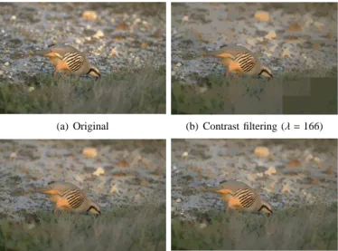
Second, we have compared attribute filtering based on a fixed threshold with the adaptive paradigm, in the context of patch-based decomposition. The contrast attribute of a node has been defined as maxp,q∈XkI(p) − I(q)k1 where X denotes the support (full connected component) of the node and k. − .k1 is the L1 distance. Fig. 3 illustrates a comparison between contrast filtering based on a fixed threshold (b) and adaptive

1_{http://qt.digia.com}

2_{http://code.google.com/cgraph}

(a) Original (b) Filtered (118 patches, α = 0.5)

(c) Original (d) Filtered (13 patches, α = 0.3)

Fig. 2. Adaptive area filtering in the RGB space. All images are part of the Berkeley Segmentation Image Dataset (https://www.eecs.berkeley.edu/ Research/Projects/CS/vision/bsds).

filtering based on an adaptive threshold with similar behaviour in the textural part of the bird (d). Both filterings have been performed in 13 overlapping patches. It can be observed that in Fig. 3(b), the tilling effect due to the decomposition into patches is visible while it is not in Fig. 3(d).

(a) Original (b) Contrast filtering (λ = 166)

(c) Adaptive area filtering (α = 0.5) (d) Adapt. contrast filtering (α = 0.5)

Fig. 3. Area and contrast filtering in the RGB space. Filtering was performed in 13 overlapping patches.

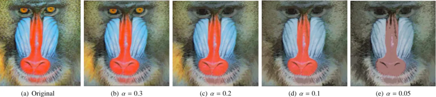
The HSV (Hue/Saturation/Value) colour space has a more perceptual meaning than RGB, since its purpose is to decor-relate hue (which can be considered as a set without obvious ordering) from saturation (which characterizes colour “purity”) and value (which gives the degree of “brightness” of the colour). Therefore a straightforward use of this colour space consists of computing the component-graph using only the S and V components while restoring the original H in the filtered

(a) Original (b) α = 0.3 (c) α = 0.2 (d) α = 0.1 (e) α = 0.05

Fig. 4. Adaptive area filtering in the Saturation Value space for decreasing values of α.

Fig. 5. Comparison of time between tree (in blue), component-graph (in purple) and multithreaded component-component-graph (in orange) computation. The multithreaded version uses a decomposition in 25 patches with one thread per patch.

image. Based on this method, Fig. 4 illustrates an adaptive area filtering on the SV space for decreasing values of α.

The processing times for component-tree (using grayscale version of the images), component-graph and multithreaded component-graph computation (using a decomposition into 25 patches) have been compared for increasing image sizes (see Fig. 5) on a Quad Core Intel Xeon CPU W3550 3.07 GHz with 4 GB of RAM. In these experiments the actual complexity for the ¨G computation was O(|Ω|1.5_{) (that is practically less} than the theoretical complexity O(|Ω|2_{). These experiments} confirm that patch decomposition enables to obtain acceptable processing times.

Future works will address the algorithmic and memory complexity of G and ˙G computation by considering paral-lel/distributed computing [22]. Multivalued image segmen-tation will also be explored, by considering for example segmentation based on optimal cuts [23], [24].

REFERENCES

[1] L. Najman and H. Talbot, Eds., Mathematical Morphology: From

Theory to Applications. ISTE/J. Wiley & Sons, 2010.

[2] H. J. A. M. Heijmans, “Theoretical aspects of gray-level morphology,”

IEEE T Pattern Anal, vol. 13, pp. 568–582, 1991.

[3] E. Aptoula and S. Lefèvre, “A comparative study on multivariate mathematical morphology,” Pattern Recogn, vol. 40, pp. 2914–2929, 2007.

[4] P. Salembier and J. Serra, “Flat zones filtering, connected operators, and filters by reconstruction,” IEEE T Image Process, vol. 4, pp. 1153–1160, 1995.

[5] P. Salembier and M. H. F. Wilkinson, “Connected operators: A review of region-based morphological image processing techniques,” IEEE Signal

Proc Mag, vol. 26, pp. 136–157, 2009.

[6] P. Salembier, A. Oliveras, and L. Garrido, “Anti-extensive connected operators for image and sequence processing,” IEEE T Image Process, vol. 7, pp. 555–570, 1998.

[7] P. Monasse and F. Guichard, “Scale-space from a level lines tree,” J

Vis Commun Image R, vol. 11, pp. 224–236, 2000.

[8] P. Salembier and L. Garrido, “Binary partition tree as an efficient representation for image processing, segmentation and information retrieval,” IEEE T Image Process, vol. 9, pp. 561–576, 2000. [9] P. Soille, “Constrained connectivity for hierarchical image partitioning

and simplification,” IEEE T Pattern Anal, vol. 30, pp. 1132–1145, 2008. [10] L. Najman and T. Géraud, “Discrete set-valued continuity and inter-polation,” in ISMM, ser. Lect Notes Comput Sc, vol. 7883, 2013, pp. 37–48.

[11] C. Kurtz, B. Naegel, and N. Passat, “Multivalued component-tree filtering,” in ICPR, 2014.

[12] N. Passat and B. Naegel, “Component-hypertrees for image segmen-tation,” in ISMM, ser. Lect Notes Comput Sc, vol. 6671, 2011, pp. 284–295.

[13] O. Tankyevych, H. Talbot, and N. Passat, “Semi-connections and hierarchies,” in ISMM, ser. Lect Notes Comput Sc, vol. 7883, 2013, pp. 157–168.

[14] B. Naegel and N. Passat, “Component-trees and multivalued images: A comparative study,” in ISMM, ser. Lect Notes Comput Sc, vol. 5720, 2009, pp. 261–171.

[15] N. Passat and B. Naegel, “An extension of component-trees to partial orders,” in ICIP, 2009, pp. 3981–3984.

[16] ——, “Component-trees and multivalued images: Structural properties,”

J Math Imaging Vis, vol. 49, no. 1, pp. 37–50, 2014.

[17] E. Carlinet and T. Géraud, “A comparison of many max-tree computa-tion algorithms,” in ISMM, ser. Lect Notes Comput Sc, vol. 7883, 2013, pp. 73–84.

[18] E. J. Breen and R. Jones, “Attribute openings, thinnings, and granu-lometries,” Comput Vis Image Und, vol. 64, pp. 377–389, 1996. [19] R. Jones, “Connected filtering and segmentation using component

trees,” Comput Vis Image Und, vol. 75, pp. 215–228, 1999.

[20] B. Naegel and N. Passat, “Toward connected filtering based on component-graphs,” in ISMM, ser. Lect Notes Comput Sc, vol. 7883, 2013, pp. 350–361.

[21] A. V. Aho, M. R. Garey, and J. D. Ullman, “The transitive reduction of a directed graph,” SIAM J Comput, vol. 1, pp. 131–137, 1972. [22] M. H. F. Wilkinson, H. Gao, W. H. Hesselink, J.-E. Jonker, and

A. Meijster, “Concurrent computation of attribute filters on shared memory parallel machines,” IEEE T Pattern Anal, vol. 30, pp. 1800– 1813, 2008.

[23] L. Guigues, J.-P. Cocquerez, and H. Le Men, “Scale-sets image analy-sis,” Int J Comput Vision, vol. 68, pp. 289–317, 2006.

[24] J. Serra, “Tutorial on connective morphology,” IEEE J Sel Top Signal, vol. 6, pp. 739–752, 2012.