Diversity-Preserving K-Armed Bandits, Revisited
Texte intégral
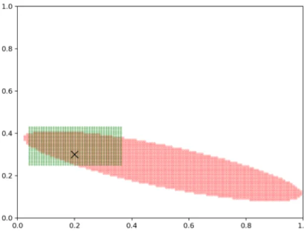
Figure
Documents relatifs
The Explore-then-Commit algorithm starts by exploring all arms m times (i.e., during the first mK rounds) before choosing the action maximizing µ b i (mK) for the remaining
This paper focuses on the case of many-armed bandits (ManAB), when the number of arms is large relatively to the relevant number N of time steps (relevant horizon) (Banks..
The second one, Meta-Bandit, formulates the Meta-Eve problem as another multi-armed bandit problem, where the two options are: i/ forgetting the whole process memory and playing
In this paper, we consider a 3-shock wave, because a 1-shock wave can be handled by the same method.. For general hyperbolic system with relaxation, the existence of the shock
Our algorithm will be competitive when applied to (and compared to algorithms specifically designed for) the continuum-armed bandit problem when there are relatively many
Assuming the knowledge of the horizon, we thus propose a computationally more efficient variant of the basic algorithm, called truncated HOO and prove that it enjoys a regret
AdaFTRL with Tsallis Entropy in the Case of a Known Payoff Upper Bound M In this section we describe how the AdaHedge learning rate scheme can be used in the FTRL framework with
We have shown that, when covariates describing those actions are uniformly distributed in [0, 1], the expected reward function m satisfies Assumption 2 and 3, and the budget
