Optimal Glideslope Guidance Algorithm for Minimum-Fuel Fixed-Time Elliptic Rendezvous

For any given dimension, we prove the existence of an optimal subspace of at most that dimension which realizes the best approx- imation –in mean parametric norm associated to

In this paper, a fuel optimal rendezvous problem is tackled in the Hill-Clohessy-Wiltshire framework with several operational constraints as bounds on the thrust, non linear non

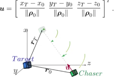
Abstract: This paper focuses on the fixed-time minimum-fuel out-of-plane rendezvous between close elliptic orbits of an active spacecraft, with a passive target spacecraft, assuming

From a second- order consensus algorithm applied to a leader-follower formation control, we (i) develop a broadcast-based network protocol able to obtain single-hop consensus in

This algorithm combines an original crossover based on the union of independent sets proposed in [1] and local search techniques dedicated to the minimum sum coloring problem

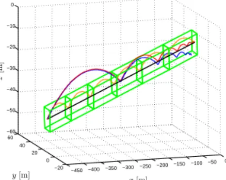
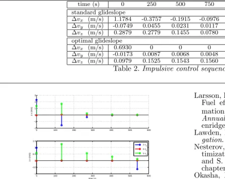
In the context of a chemical propulsion, the classical multipulse glideslope algorithm of Hablani is revisited and it is shown that when considering specific common directions for

The main result of the paper is now presented. It mainly consists in identifying some degrees of freedom and deriving a numerically tractable expression for the different constraints

Applying the maximum Principle to the original optimal control problem (5) for a fixed number of impulses and under the impulsive approximation as described in Lawden [15], or