Publisher’s version / Version de l'éditeur:
Cold Regions Science and Technology, 41, February 2, pp. 83-89, 2005-02-01
READ THESE TERMS AND CONDITIONS CAREFULLY BEFORE USING THIS WEBSITE.
https://nrc-publications.canada.ca/eng/copyright
Vous avez des questions? Nous pouvons vous aider. Pour communiquer directement avec un auteur, consultez la
première page de la revue dans laquelle son article a été publié afin de trouver ses coordonnées. Si vous n’arrivez pas à les repérer, communiquez avec nous à [email protected].
Questions? Contact the NRC Publications Archive team at
[email protected]. If you wish to email the authors directly, please see the first page of the publication for their contact information.
Archives des publications du CNRC
This publication could be one of several versions: author’s original, accepted manuscript or the publisher’s version. / La version de cette publication peut être l’une des suivantes : la version prépublication de l’auteur, la version acceptée du manuscrit ou la version de l’éditeur.
For the publisher’s version, please access the DOI link below./ Pour consulter la version de l’éditeur, utilisez le lien DOI ci-dessous.
https://doi.org/10.1016/j.coldregions.2004.07.004
Access and use of this website and the material on it are subject to the Terms and Conditions set forth at
A Note on electrical freezing and shorting potentials Parameswaran, V. R.; Burn, C. R.; Profir, A.; Ngo, Q.
https://publications-cnrc.canada.ca/fra/droits
L’accès à ce site Web et l’utilisation de son contenu sont assujettis aux conditions présentées dans le site LISEZ CES CONDITIONS ATTENTIVEMENT AVANT D’UTILISER CE SITE WEB.
NRC Publications Record / Notice d'Archives des publications de CNRC:
https://nrc-publications.canada.ca/eng/view/object/?id=69e36e21-5644-4dee-be9b-edea3f7a150b https://publications-cnrc.canada.ca/fra/voir/objet/?id=69e36e21-5644-4dee-be9b-edea3f7a150b
A Note on electrical freezing and shorting potentials
Parameswaran, V.R.; Burn, C.R.; Profir, A.; Ngo, Q.
NRCC-47671
A version of this document is published in / Une version de ce document se trouve dans: Cold Regions Science and Technology, v. 41, no. 2, Feb. 2005, pp. 83-89
Doi: 10.1016/j.coldregions.2004.07.004
A NOTE ON ELECTRICAL FREEZING AND SHORTING POTENTIALS
V. R. (Sivan) Parameswaran1, C. R. Burn2, Aileen Profir3 and Quang Ngo4 Department of Geography and Environmental Sciences
Carleton University, Ottawa, Ontario, Canada ABSTRACT
Electrical potentials developed by charge separation during freezing of water and
dilute CaCl2 solutions were studied in the laboratory, using gold-plated copper electrodes
placed across the freezing boundary. A sudden increase in the potential occurs when the
freezing front reaches an electrode. A shorting potential was observed at the electrodes
when the freezing front advanced past the reference electrode. The magnitude of the
freezing and shorting potentials is of the order of a few hundred millivolts. This
technique can be used to detect and monitor the movement of freeze-thaw boundaries in
water and moist soils.
[Key Words: Freezing, Potentials, Electrodes, Interface, Freeze-Thaw Boundary]
Introduction:
An electrical potential develops across a freezing interface in aqueous solutions
and moist soils due to charge separation and preferential entrapment of ions in the two
different phases (Workman and Reynolds 1950; Parameswaran and Mackay 1996). The
magnitude of the potential depends on various factors including the rate of cooling and
species and concentration of solute present in the solution or soil. Under normal rates of
cooling experienced in nature, the freezing potentials measured are in the range of a few
millivolts. Under fast cooling using very cold circulating baths, potentials of several volts
1
Adjunct Professor, also Guest Researcher, Institute for Research in Construction, National Research Council Canada, Ottawa, Ontario K1A 0R6, Canada; to whom all correspondence should be addressed;
2
have been measured (Workman and Reynolds, 1950; Gill and Alfrey, 1952). The wide
range of values of freezing potentials observed in solutions by different authors under
similar conditions, indicates that the measured potential depends on various factors such
as the purity of the solution, the experimental set up, including the type of electrodes and
wires used, the connection to the measuring/recording equipment, internal resistance of
the recorder, and so forth. Pressure also has an effect on the development of potentials,
especially in soils, where frost heaving is commonly observed (Kelsh and Taylor, 1988).
The magnitude of the potentials measured by various authors has varied over three orders
of magnitude, 100 mV to 230 V (Workman and Reynolds, 1950; Pruppacher, et al., 1968;
Cobb and Gross, 1969; Murphy, 1970). In pure water, the values of the freezing
potentials measured were between 200 mV and 120 V (Arabadzhi, 1948; Workman and
Reynolds, 1950; Gill and Alfrey, 1952; Bayadina, 1960; Murphy, 1970; Korkina, 1975;
Parameswaran, 1982).
Fortier et al. (1993), measured the electrical potential developed across a thawing
boundary in the active layer of permafrost in Umiujaq in Nunavic, located on the east
coast of Hudson Bay, in the Arctic regions of Quebec. They used a reference electrode
located deep in the unfrozen ground and the potentials developed on each electrode above
that were measured. The potentials measured were interpreted as a combination of
freezing potentials, streaming potentials due to water migration and changes in the
electrolyte concentration. They concluded that by monitoring these potential differences,
changes in temperature, water content and migration and ionic distribution can be
Outcalt and his co-workers (1989, 1990) carried out combined measurements of
soil temperature and electric potential in the seasonally freezing top layer of a sandy loam
soil at a site in the Botanical Garden inUniversity of Michigan, Ann Arbor. They
measured electric potentials of 300 to 700 mV and interpreted the data as the result of
thermally induced ionic concentration in the soil. They suggested that secondary effects
due to advective flow of water to the freezing front (streaming potential) could also give
rise to electric potentials. They concluded that valuable information on the geotechnical
conditions of freezing soils (the state and mobility of the soil water) can be gathered by
combining thermal and electrical potential measurements.
Past measurements in the laboratory and in the field indicate that the potentials
developed during freezing of water and soils containing ionic impurities in solution, are
on the order of a few hundred millivolts (Parameswaran, et al., 1982, 1983, 1985, 1996;
Burn et al., 1998). Field measurements near the western Arctic coast of Canada include
those carried out in the lakes near Inuvik, pingos and at the bottom of a drained lake of
the Tuktoyaktuk Peninsula area where permafrost was aggrading. The ionic impurities in
these systems consisted mainly of cations: Ca++, Mg++, K+ and Na+ and the anion, Cl-. For
example, the drill hole water from Pingo 9 contained 230 – 260 ppm of Ca++, 85-95 ppm
Mg++ and about 250 ppm Cl-, besides small amounts of K+ and Na+. The water from the
Inuvik lakes contained 16-30 ppm Ca++, 5-8 ppm Mg++, and less than 10 ppm each of Na+
and K+.
These measurements showed a finite potential difference between an electrode
located at the freezing interface and a reference electrode in the unfrozen region. These
freezing/thawing interfaces in the ground. An experimental program was set up to
systematically study freezing potentials developed in different solutions and at different
freezing rates.
Experimental Set-Up
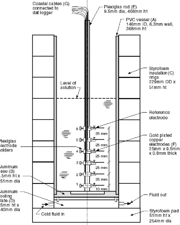
Fig. 1 shows a schematic diagram of the experimental cell. This consisted of a
cylindrical PVC vessel (A) of internal diameter, 146 mm (5.75" nominal), height 368 mm
(14.5"), wall thickness 6.3 mm and closed at one end with an aluminum base (B). The
cylinder was insulated with Styrofoam rings (C) of thickness 51 mm. The cylinder was
placed on a cooling chamber (D) through which a cold fluid (Prestone antifreeze) could
be circulated. The cooling plate had inlet and outlet PVC tubes connected to a Haake G
cooling bath with a Haake D8 temperature controller. The temperature of the bath could
be controlled to + 0.1oC accuracy. A Plexiglas rod (E) of diameter 9.5 mm (0.375") and
length, 406 mm and containing 6 electrodes in the form of gold-plated copper strips (F),
(25 mm X 9.5 mm X 0.8 mm thickness) was placed at the center of the cylinder. The
copper strip electrodes were parallel to the base of the cell. The bottom electrode was 10
mm above the bottom of the vessel and the others were positioned at 25 mm intervals.
Thermistors (Beta Therm 2.2K3A1A) were also attached at each electrode location.
Coaxial cables (G) were soldered to the electrodes and thermistors and connected to an
external data logging system (Campbell Scientific Inc. Model CR 10). The time,
temperature and electrical potentials were measured by the recorder every 5 minutes and
averaged every 15 minutes and the data was stored in a storage module SM192 attached
The CR-10 data logger has an internal impedence of 200 giga ohms (2 x 10⁹Ω), sufficiently large to measure even very small potential differences. Resolutionof the
instrument in the 10 mV scale is 0.33 µV and in the 2500 mV range, 0.33 mV. The top electrode used as the reference electrode was connected to the ground terminal of the
instrument and the lower five electrodes were connected to the terminals 1 to 5, starting
from the bottom electrode upwards.
Experimental Procedure
Experiments were carried out to measure the freezing potentials in the following liquids:
a) de-ionized water, boiled to remove dissolved gases, in particular, CO2;
b) de-ionized, boiled water with CaCl2 at concentrations of 20, 40 and 60 ppm.
CaCl2 was chosen as a solute for the experiments, as it is one of the main constituents in
the field solutions we continue to study. No reliable data for potentials developed during
freezing of CaCl2 solutions are available other than those of Workman and Reynolds
(1950).
The PVC cylindrical vessel with the electrode stand positioned in the center was
placed on the cooling plate inside an incubator maintained at 4oC. The liquid was poured
in the vessel to a height just above the top electrode, and the column was frozen from the
bottom upwards. The top electrode remaining in the unfrozen water (until the freezing
front reaches the top) was the reference electrode against which the potentials developed
in all the other electrodes were measured. The time, temperature and voltage developed at
each electrode were scanned every 5 minutes and averaged every 15 minutes and the data
Figure 2 shows the potentials developed at two different electrode locations in
de-ionized water. The circulating bath temperature was -10o C. Fig. 2(a) shows a sharp peak
F, when the freezing front reached the electrode-3 The absolute magnitude of this
freezing potential was about 75 mV, as measured from the beginning to the end of the
straight line portion of the jump in voltage (a drop in potential from –50 to –125 mV). As
the freezing front advanced to reference electrode-6, a reverse potential (hereafter called
the "Shorting Potential" and indicated by "S") of about 100 mV was measured, from the
beginning to the end of the straight line portion of the jump (from
–25 to +75 mV). In Fig. 2(b) similar jumps in the potential are seen on electrode-5, but
the two peaks are closer to each other, as electrode-5 was just below electrode-6. The
magnitude of the potentials were of the same order as those observed at the electrode
location 3.
Figures 3(a) and 3(b) show, the potentials developed in a solution of CaCl2 in
de-ionized water, at -10oC and -15oC, respectively. The pattern is similar to that seen in Fig.
2, but at -15oC, the peaks of freezing and shorting potentials are sharper, meaning, the
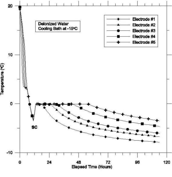
rise and fall of the potential is steep and not gradual. Figures 4 and 5 show respectively,
the temperatures and the potentials developed at each electrode, in an experiment with
distilled water, with the circulating bath fluid at –15o C. The initial dip in temperature
below 0oC, seen in Fig. 4 (indicated by the arrow, SC), is due to supercooling of the
solution, before normal freezing starts. [Note: The occurrence of supercooling was not a
regular phenomenon in all experiments. For supercooling to occur, the system has to be
in perfectly still condition with no vibration or nucleating agents present in the solution.
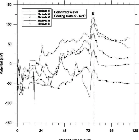
Fig. 5 shows the variation of the potential difference at all electrodes, with respect to the
top reference electrode. There is also a gradual increase in the potential difference after
the onset of freezing at each electrode, as the temperature at that location drops with the
progress of the cooling, until the freezing front touches the top reference electrode (No.
6). At this time the system is completely frozen and both the measuring and reference
electrodes are embedded in solid ice, essentially shorting the system. The simultaneous
occurrence of the shorting potential at all electodes at the instant the freezing front
touches the top reference electrode, is seen in Figure 5, as indicated by the peaks
occurring at “S”, the vertical dashed line at 78 hours.
The data show the following:
a) As the freezing front touches each electrode, an abrupt change in potential (measured
with respect to the top electrode in the unfrozen liquid) occurs due to the freezing
potential associated with the phase change. The potentials measured have been
ice-negative. This decays as the freezing front passes the particular electrode.
b) As the freezing front advances beyond the uppermost electrode, the voltage-time
curve shows a spike (abrupt change in potential) caused by shorting of the system.
The magnitude of this “shorting potential” peak may be of the same order, but of
opposite sign, . as the first freezing potential observed at that electrode.
c) Once the entire bath in the cell is completely frozen, the temperature begins to drop at
each electrode and a temperature differential is set up between the top electrode and
each of the lower electrodes. This temperature differential causes the development of
a small potential due to charge separation caused by the temperature gradient, as
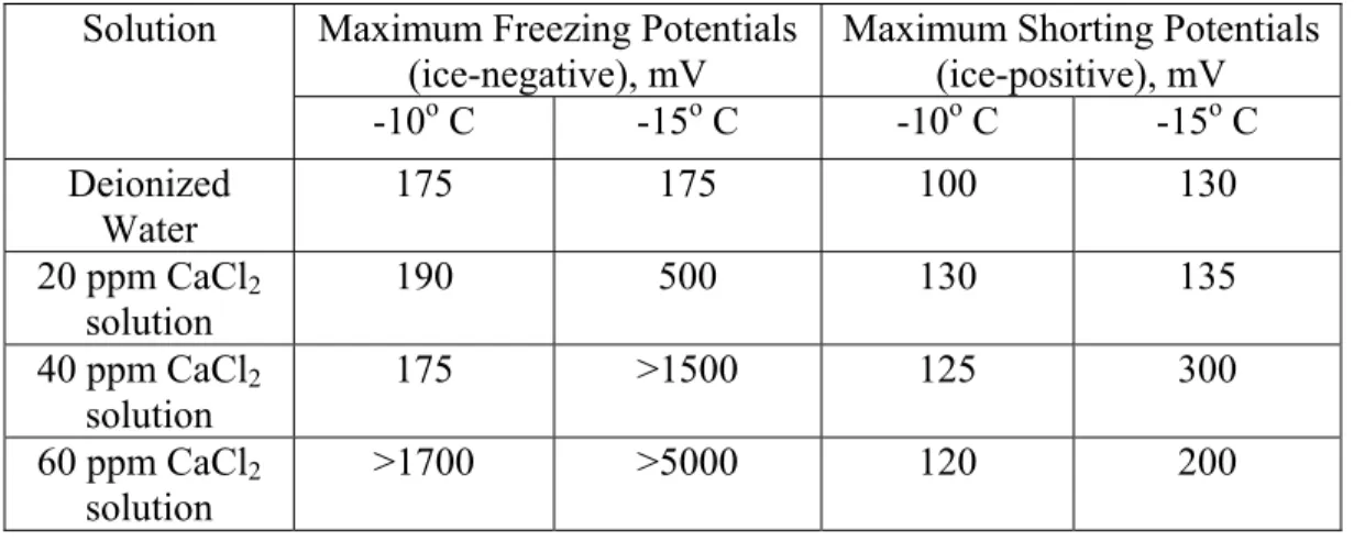
Table 1 shows the maximum values of the freezing potentials and "shorting
potentials" observed in each solution in this series of experiments. In general, the freezing
potentials are higher with faster rate of cooling using a colder circulating bath. Ionic
impurities increase the magnitude of the potentials.
Discussion
The freezing potentials measured in the present experiments were ice-negative
and the “shorting potentials” were ice positive. These are potential differences measured
between each of the lower electrodes as the freezing front touches that electrode and the
reference electrode in the unfrozen liquid, assuming that the environment around this
reference electrode remains unchanged. This may not actually be the case, especially in
ionic solutions, as there will be solute rejection at the freezing interface and the
concentration of the unfrozen liquid may change, although slightly. Attempts have been
made by different authors, to use an external ground electrode as the reference electrode
(in particular, in field measurements) against which the potentials at all electrodes were
measured. Even in such cases, stray currents through the ground as well as diurnal
changes in temperature and atmospheric conditions could affect magnitude of the
potential difference developed between the electrodes.
The results from the present experiments show the onset of a freezing potential on
an electrode located at the freezing boundary and is a definite indication of the arrival of
the freezing front at that electrode location. The absolute magnitude of the potential will
depend on several factors such a the quality of the solution, physical characteristics of the
point is that the present technique using electrodes does indicate the time of arrival of the
freezing front at each location and from this, the rate of advance of a freezing boundary
can be accurately determined.
A potential difference can also arise due to the thermal gradient within the ice
(Latham et al., 1981). This is mainly due to the concentration gradients of H+ and OH
-ions set up under the temperature gradient. The gradual increase in the measured potential
at different electrodes, shown in Fig. 5, is an indication of this. In ionic solutions a
concentration gradient of ions could also arise by rejection of solute to the unfrozen water
at the freezing boundary and this could also give rise to the gradual rise in potential.
The observation of a "Shorting Potential", as the freezing front advances past the
reference electrode, has not been reported before. This shorting potential arises from
charge equalization throughout the ice. The shorting potential is observed at all electrodes
simultaneously, when the freezing front passes the reference electrode at the top of the
column. In Figure 5, the peaks due to the shorting potentials on all electrodes occur at
the same time, about 78 hours after the beginning of the experiment.
The freezing and shorting potentials indicate respectively, the onset of freezing
and the completion of freezing of a solution below the reference electrode. Since the
potential jumps are quite sharp and instantaneous, this could be used as an accurate
method to monitor and measure the progress of freezing in a solution.
Acknowledgements
The authors are very thankful to the referees for their thorough review and their
Conclusions
1. Electrical potentials are generated due to charge separation and preferential
accumulation in the two phases of a freezing solution. This can be noticed as an
instantaneous shift in the DC voltage measured between an electrode at the freezing
interface and a reference electrode in the unfrozen solution.
2. The magnitude of the freezing potentials are higher at faster rates of cooling
produced by a cooler circulating bath.
3. Dilute solutions of CaCl2 generate higher freezing potentials than pure water, the
magnitude of the potential being higher for the higher concentration.
4. A shorting potential is recorded at the instant the freezing front passes the reference
electrode. The magnitude of this shorting potential is of the same order as that of the
freezing potential.
5. By measuring the freezing and shorting potentials, the progress of freezing can be
References:
1. Arabadzhi, V. I. (1948). Contact potential differences between water and ice. Reports
of the Academy of Sciences of the USSR., Vol. 60, No. 5, pp 811-812, translated by
William Mandel, SIPRE Translation No. 1, 1950.
2. Bayadina, F. I. (1960). Voltage difference originating between the solid and liquid
phases of water. IZV. In USSR Geophysical Series No. 2.
3. Burn, C. R., Parameswaran, V. R. (Sivan), Kutny, L. and Boyle, L. (1998).
Electrical potentials measured during growth of lake ice, Mackenzie Delta area,
N.W.T., Canada. 7th Int. Permafrost Conference, Yellowknife, NWT, June 1998,
Proceedings pp 101-106.
4. Cobb, A. E. and Gross, G. W. (1969). Interfacial electrical effects observed during the
freezing of dilute electrolytes in water. J. Electrochemical Society; Electrochemical
Sciences, Vol. 116, pp 796-804.
5. Fortier, R., Allard, M. and Seguin, M-K. (1993). Monitoring thawing front movement
by self-potential measurement. Permafrost, Sixth International Conference (July
1993), Proceedings Vol. 1, South China University of Technology Press, 1993, pp
182-187)
6. Gill E. W. B. and Alfrey, G. F. (1952). Production of electrical charges on water
drops. Nature, Vol. 169, pp 103-104.
7. Kelsh, D. J. and Taylor, S. (1988). Measurement and interpretation of electrical
freezing potential of soils. U. S. Army CRREL Report No. CRREL-88-10, 15 p
8. Korkina, R. I. (1975). Electrical potentials in freezing solutions and effect on
9. Latham, J and Mason, B. J. (1961). Electric charge transfer associated with
temperature gradients in ice. Proc. Roy. Soc. (London), A 260, pp 523-526.
10. Murphy, E. J. (1970). The generation of electromotive forces during the freezing of
water. J. Colloid and Interface Sci., Vol. 32, pp 1-11.
11. Outcalt, S. I., Gray, D. H. and Benninghoff, W. S. (1989). Soil temperature and
electric potential during diurnal and seasonal freeze-thaw. Cold Regions Science and
Technology, Vol. 16 , pp 37-43.
12. Outcalt, S. I. And Hinkel, K. M. (1989). Night-frost modulation of near-surface
soil-water ion concentration and thermal fields. Physical Geography, Vol. 10, No. 4, pp
336-348
13. Outcalt, S. I. And Hinkel, K. M. (1990). The soil electric potential signature of
summer draught. Theor. And Appl. Climatology, Vol. 41, pp 63-68.
14. Parameswaran, V. R. (1982) Electrical freezing potentials in water and soils. Third
Int. Symp. On Ground Freezing, Hanover, NH, June 1982, ISGF - Vol-II, pp 83-89.
15. Parameswaran and Mackay, J. R. (1983). Field measurements of electrical freezing
potentials in permafrost areas. Permafrost: Fourth International Conference,
Fairbanks, Alaska, July 1983, Proceedings pp 962-967.
16. Parameswaran, V. R., Johnston, G. H. and Mackay, J. R. (1985). Electrical potentials
developed during thawing of frozen ground. Fourth Int. Symp. on Ground Freezing,
Sapporo, Japan, August 1985, Proceedings Vol. I, pp 9-16.
17. Parameswaran, V. R. and Mackay, J. R. (1996) Electrical freezing potentials
measured in a pingo growing in the western Canadian Arctic. Cold Regions Science
18. Pruppacher, H. R., Steinberger, E. H. and Wang, T.L (1968). On the electrical effects
that accompany the spontaneous growth of ice in supercooled aqueous solutions.
J. Geophys. Res., Vol. 73, pp 571-584.
19. Workman, E. J. and Reynolds, S. E. (1950). Electrical phenomena occurring during
the freezing of dilute aqueous solutions and their possible relationship to
Table 1. Maximum values of freezing and shorting potentials measured in the present experiments.
Maximum Freezing Potentials (ice-negative), mV
Maximum Shorting Potentials (ice-positive), mV Solution -10o C -15o C -10o C -15o C Deionized Water 175 175 100 130 20 ppm CaCl2 solution 190 500 130 135 40 ppm CaCl2 solution 175 >1500 125 300 60 ppm CaCl2 solution >1700 >5000 120 200
Figure Captions:
Fig. 1. Experimental cell to measure electrical freezing potentials in solutions
Fig. 2. Freezing potentials developed in de-ionized water, with the circulating bath
temperature at -10oC. The first negative peak (F) indicates the onset of freezing
and the next positive peak (S) denotes the shorting potential.
(a) Electrode 3; (b) Electrode 5.
Fig. 3. Freezing Potentials developed at electrode 3, using a solution of CaCl2 (20 ppm)
in de-ionized water. Circulating bath temperature: (a) -10oC; (b) -15oC.
Fig. 4. A typical chart showing the variation of the temperature with time, at different
Electrodes. The arrow (SC) indicates supercooling
Fig. 5. A typical chart, showing the simultaneous occurrence of shorting potential (S) at
Figure 2(a). Freezing potentials developed in de-ionized water, with the circulating bath temperature at –10oC, at electrode-3. The first negative peak (F) indicates the onset of freezing and the next positive peak (S) denotes the shorting potential
Figure 2(b). Freezing potentials developed in de-ionized water, with the circulating bath temperature at –10oC, at electrode-5. The first negative peak (F) indicates the onset of freezing and the next positive peak (S) denotes the shorting potential
Figure 3(a). Freezing potentials developed at electrode-3 using a solution of CaCl2 (20 ppm) in de-ionized water.
Figure 3(b). Freezing potentials developed at electrode-3 using a solution of CaCl2 (20 ppm) in de-ionized water.
Figure 4. A typical chart showing the variation of temperature with time at different electrodes.
Figure 5. A typical chart showing the simultaneous occurrence of Shorting potential (S) at all electrode locations.