HAL Id: inserm-00858075
https://www.hal.inserm.fr/inserm-00858075
Submitted on 4 Sep 2013
HAL is a multi-disciplinary open access
archive for the deposit and dissemination of
sci-entific research documents, whether they are
pub-lished or not. The documents may come from
teaching and research institutions in France or
abroad, or from public or private research centers.
L’archive ouverte pluridisciplinaire HAL, est
destinée au dépôt et à la diffusion de documents
scientifiques de niveau recherche, publiés ou non,
émanant des établissements d’enseignement et de
recherche français ou étrangers, des laboratoires
publics ou privés.
resonance imaging
Teodora-Adriana Perles-Barbacaru, Hana Lahrech
To cite this version:
Teodora-Adriana Perles-Barbacaru, Hana Lahrech. Quantitative mapping of angiogenesis by magnetic
resonance imaging. Functional Brain Mapping and the Endeavor to Understand the Working Brain,
InTech, pp.457-511, 2013. �inserm-00858075�
Quantitative Mapping of Angiogenesis by Magnetic
Resonance Imaging
Teodora-Adriana Perles-Barbacaru and
Hana Lahrech
Additional information is available at the end of the chapter http://dx.doi.org/10.5772/56492
1. Introduction
Since tumors are commonly associated with angiogenesis and compromised vascular wall integrity, the ability to focus noninvasive imaging techniques on vascular characteristics provides a physiologically-specific approach to tumor delineation which is of utility in guiding the biopsy and in surgical or radiation treatment planning. Hypervascularisation mapped by magnetic resonance imaging (MRI) correlates with histologically-assessed tumor grade [1]. It is also of value in distinguishing residual or recurrent tumor from treatment effects such as radiation induced necrosis [2]. Furthermore, by quantitatively assessing tumor vascularity and endothelial permeability, these approaches allow the evaluation of novel anti-angiogenic therapies, guiding drug development through preclinical stages, and facilitate the inter- and intra-subject comparisons. They also allow the assessment of the biological efficacy of therapies in the clinical setting, before more traditional criteria, such as tumor size change, become apparent. This is particularly important with novel antiangiogenic agents to distinguish potential responders from nonresponders.
This chapter focuses on MRI techniques for angiogenesis assessment. In particular it describes a newly developed quantitative MRI technique for in vivo blood volume fraction mapping for preclinical and above all for clinical applications in neurooncology. The blood volume fraction is a biomarker for angiogenesis and has proven successful in mapping brain dysfunction and in testing drug efficacy. The described technique is compared with other magnetic resonance imaging techniques currently employed in the preclinical and clinical setting. Therefore, this chapter provides an overview of existing quantitative MRI techniques, briefly explains their basic principle, states their acquisition and postprocessing requirements, and compares their advantages and limits. Quantitative results for blood volume fraction measures in laboratory
© 2013 Perles-Barbacaru and Lahrech; licensee InTech. This is an open access article distributed under the terms of the Creative Commons Attribution License (http://creativecommons.org/licenses/by/3.0), which permits unrestricted use, distribution, and reproduction in any medium, provided the original work is properly cited.
animals and human subjects are presented and compared. Pitfalls and possibilities in neuro‐ oncological applications are pointed out and discussed.
2. When and why do we need to image angiogenesis?
The vasculature of brain tissue is a complex entity having multiple functions and regulatory mechanisms. One of its functions is to maintain and adjust the blood supply to meet the energy demands of the brain tissue. Most adjustments occur at the microscopic level. Tissues with a high metabolic turnover are generally equipped with a more extensive network of microves‐ sels. Tumor growth and metastasis depend on tumor-induced angiogenesis, i.e. cancer cells with increased metabolism attract and maintain a blood supply [3, 4].
Brain capillaries are composed of a unique and continuous layer of endothelial cells connected by adhesion proteins. In addition, pericytes and foot like processes of astrocytes surround the basal lamina. This forms a regulatory interface between the blood and the cerebral parenchy‐ ma: the blood brain barrier (BBB). It is impermeable to many water soluble macromolecules, including many drugs and magnetic resonance contrast agents (CAs). However, the BBB is disrupted in many pathologic processes that involve inflammation or neovascularisation such as tumor growth.
Angiogenesis in malignant tumor tissue is structurally and functionally different from physiologic angiogenesis occurring during fetal development or tissue repair. The microvas‐ cular architecture is characterized by tortuous vessels with varying diameter, abnormal branching pattern and blind ending protrusions. Fast growing tumor vasculature is usually immature and lacks the regulatory mechanisms and competent BBB. This leads to a heteroge‐ neous perfusion with parts of the tumor that are hyperperfused due to high microvascular density, and other parts that are hypoperfused with a low proportion of functional vessels. Blood turbulence and stasis as well as endothelial dysfunction lead to thrombosis. Remaining vessels may enlarge in an effort to compensate for the reduced blood flow. The resulting tissue hypoxia triggers secretion of angiogenic factors which maintain the angiogenic process [5]. Hyperpermeability of the incompetent BBB to macromolecules leads to edema and increased interstitial pressure which in turn may impede delivery of therapeutic agents to the tumor tissue.
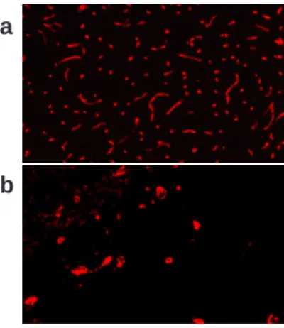
Figure 1 shows representative vessel sections from healthy rat brain tissue and an experimental brain tumor.
Along with the mitotic index, presence of necrotic areas, invasive potential and cell differen‐ tiation, angiogenesis has been recognized as one of the diagnostic criterions of malignancy in the World Health Organization (WHO) classification. Similar to the presence of mitosis and necrosis, vascular proliferation is significantly correlated to survival [6-10]. Although neuro‐ radiologic features can be highly suggestive, diagnosis is based on histologic examination. Neuroradiologic mapping of angiogenesis is important to guide the biopsy needle to sample appropriate tissue. After grading is established neuroimaging techniques help to delineate the
tumor for radiotherapy and/or surgical planning. Magnetic resonance imaging (MRI) capable of multiparametric mapping and yielding high soft tissue contrast is widely used for diagnosis, surgical and radiation treatment planning as well as for treatment follow up. In many imaging facilities, perfusion MRI used to map vascular and hemodynamic parameters is part of the neuroimaging protocol, at least for diagnosis and treatment planning. In the advent of new treatment strategies targeted at the angiogenic process, noninvasive mapping of angiogenesis by MRI will become a requisite to monitor treatment efficacy in follow up studies.
3. What are imaging biomarkers of angiogenesis?
At the microscopic level, several parameters are used to describe and quantify the vascular network. Microvascular density, Nv (cm-2), simply reports the number of vessels per unit area
regardless of their shape, orientation or size. Together with the vascular volume density, which is the volume occupied by vascular walls and blood per unit volume of tissue, the microvas‐ cular density is the most frequently used parameter for angiogenesis quantification. The microvascular surface Sv is important for exchange processes between blood and interstitium
and is approximately 100 cm2g-1 tissue [11]. The length density L
v (cm-2) is the total length of
microvessels existing per unit volume of tissue. The vessel radii are important for rheological considerations because they define the cross sectional area that in turn is one of the parameters that determines the blood flow rate. The vascular area density is the ratio between the total area of vessel cross sections and the area of the region of interest (ROI) and correlates with the vascular volume density. The mean intercapillary distance in the human brain is about 40 μm [12] and is an index of the access of an interstitial cell to the exchange processes at the vascular boundary, since in the interstitium transport is mainly governed by diffusion. Other morpho‐
a
b
Figure 1. Immunofluorescent staining of collagen IV a component of the basal lamina of the vessel wall. a: Cortical
vessels in a healthy rat are delicate, with a narrow distribution of vessel radii around 8 μm and randomly oriented and homogenously distributed. b: Tumor vasculature in a C6 glioma model is composed of sparse irregularly shaped and enlarged vessels. Parts of the tumor are not perfused.
logical parameters that change under physiologic and pathologic conditions exist, e. g. the tortuosity, interbranching distance, branching angle. Typical microvasculature from mouse cortex and tumor tissue is shown in Figure 12 b.
However MRI and other medical imaging techniques, such as computed tomography (CT) or positron emission tomography (PET) are rather macroscopic techniques. Obviously the above mentioned morphometric parameters of microvessels are not directly measurable. However, some hemodynamic parameters are accessible by these imaging techniques. One of them is the regional cerebral blood volume (CBV), which is the quantity of blood in ml per 100 g tissue that participates in the supply of oxygen and nutrients and in the discharge of toxic metabolites. It is often also expressed as a volume fraction (blood volume fraction, BVf), approximates the vascular volume density reported in microscopy studies and is related to the mean vascular diameter, the microvascular density and length density all of which are altered in the angio‐ genic process occurring in tumors. The conversion factor between both units is 100 λ/ρblood ≈
93.75 where λ is the brain-blood partition coefficient and ρblood is the blood density [13]. CBV
mapping has proven successful in assessing angiogenesis to study brain dysfunction and in testing drug efficacy.
Another parameter is the cerebral blood flow (CBF), which is the amount of blood arriving and leaving the tissue of interest in a time interval. The average CBF in humans is approxi‐ mately 50 ml/min per 100g of brain tissue, while the critical threshold for neuronal function is approximately 20 ml/min per 100g. Another often reported quantity is the mean transit time (MTT), the average time required for blood to pass through the tissue volume of interest. It is related to CBV and CBF by MTT = CBV/CBF. Brain metabolism can be assessed by measuring the cerebral metabolic rate of oxygen (CMRO2) which is about 130 μmol/min per 100g.
The permeability of the microvasculature to a substance is often reported as the product of the diffusional permeability coefficient P (cm min-1) and the surface area S
v. PSv has the unit of a
volume flow per tissue mass (ml min-1 g-1). Only values averaged over the volume of the voxel
can be obtained without information about the morphology of the vasculature. Clinical studies have demonstrated the utility of this parameter for assessing malignancy and response to therapy in various tumors [14].
However, one MRI technique is sensitive to microvascular architecture, and the parameter obtained is called the vessel size index (VSI). This index is a weighted average of vessel sizes with a strong predominance of larger vessel sizes. It also depends on the vessel orientation which is assumed to be isotropic in healthy gray matter tissue, on the BVf and on the amount of contrast agent used.
Brain pathologies that are accompanied by vascular changes reflected by altered CBV, CBF, BBB permeability or combinations thereof, are brain infarction (ischemia) [15-17], multiple sclerosis [18, 19], infectious and inflammatory diseases [20], some forms of dementia such as Alzheimer's disease [21-23], acquired immune deficiency syndrome associated brain diseases [24, 25], and traumatic brain injury [26]. This chapter focuses on the quantification of tumor angiogenesis, which requires particular methodologic developments, due to the BBB perme‐ ability to most CAs.
4. Why are quantitative measures important?
Drugs targeting the angiogenic process such as inhibitors of angiogenic factors bring with them a need for an accurate means of assessing tumor angiogenesis and monitoring response to treatment. In the context of treatment monitoring comparison of values obtained at different time points are necessary. In the context of clinical trials comparisons between patients and centers need to be made.
Unfortunately, the signal intensity from most MR pulse sequences does not relate directly to any physiological parameter. Magnetic field strength, scanner parameters, sequence timing parameters, flip angle as well as image scaling, make the signal scanner dependent and comparisons between serial or multi-center studies difficult.
Procedures for data collection have to be found which are insensitive to scanner, sequence and operator influence, and which are reliable and reproducible over time and between patients. The measured parameters have to be examined for their biological meaning and related to clinically relevant quantities. In this way, changes at the microscopic level such as in cellular or microvascular structures can be detected as changes in MR parameters, such as relaxation times or magnetization transfer ratio, or as changes in diffusion and perfusion parameters at typical MR image resolutions of about 1 mm.
In theory, perfusion MRI techniques can yield quantitative hemodynamic parameters. To do so, they rely on a number of assumptions that are detailed below and require additional measurements that are either time consuming or invasive and therefore difficult in the clinical setting. In routine perfusion imaging, descriptive or semiquantitative parameters are therefore reported, some of which are discussed below. Typically, such values in the tissue of interest are reported relative to the corresponding value in a reference region, or are normalized to an average value taken from the literature. The reference region is chosen in healthy appearing brain tissue, usually in white matter or in the contralateral hemisphere symmetrical to the lesion. This is a pitfall when there is no reference region because the disease affects the whole brain such as a systemic cardiovascular pathology or a generalized infection, or when the “healthy appearing” reference region is affected by the disease, such as might occur with brain tumors that exert a mass effect, or have infiltrated the reference region.
5. What are the available quantitative magnetic resonance imaging
techniques?
The perfusion MRI techniques that are presently used in the clinical practice are so called dynamic techniques. Dynamic techniques involve serial acquisition of MR images before, during and after the pass of an intravenously injected exogenous MRI CA through the tissue. As the CA enters into the tissue under investigation, the T1 and T2 values of tissue water
5.1. First pass or bolus tracking techniques
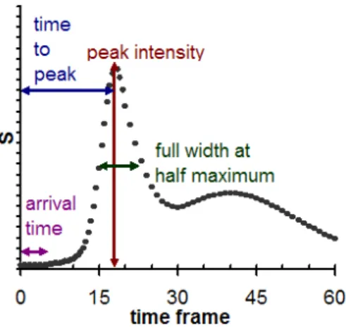
During the first pass of the CA bolus through the brain tissue the signal displays a characteristic intensity time course, which is related to the CA concentration in the tissue. Such a signal intensity time course is illustrated in Fig. 2 as an example of a positive (T1 weighted) signal
change. When changes in transverse relaxivity are exploited this technique is termed dynamic susceptibility contrast (DSC) MRI, which has superior signal to noise ratio (SNR) compared to T1 weighted techniques. Mixed T1 and T2 weighting can complicate the interpretation. Fast
imaging techniques with a recommended time resolution below 1.5 s are required, to ade‐ quately sample the signal dynamics. Even when using echo planar imaging (EPI) techniques, this requirement imposes limits to the spatial resolution and the number of slices that can be acquired.
Characteristic descriptive parameters measured form the observed signal changes during bolus pass include arrival time of the bolus, peak intensity, time to peak and full width at half maximum (Fig. 2). They generally depend on combinations of physiologic parameters, such as blood flow, fractional blood volume, and CA extravasation. Nevertheless, the peak signal amplitude was shown to correlate with the CBV [27].
For CBV quantification, the signal intensity during bolus pass is converted into a change in R1 [28], R2 or R2* [29] versus time reflecting the CA concentration. However, the proportionality
constant between tissue relaxation rate change and CA concentration not only depends on CA properties and magnetic field strength. In particular the transverse relaxivity also depends on tissue properties such as microvascular architecture, vascular permeability, water exchange rate between intra- and extracellular compartment and blood oxygenation, all of which are spatially variable. The relaxivity is generally assumed to be the same as in plasma or venous blood. Any non-linearity between relaxation rate or signal change and CA concentration in tissue and blood will lead to errors [30].
Figure 2. Characteristic signal intensity (S) time course during CA bolus passage. After the first high peak, the second
In clinical routine, the CBV in the tissue of interest is given relative to a reference tissue. Maps of relative CBV are calculated by integrating the area under the CA concentration change during the first pass over time and since the CBV is calculated on the basis of signal recovery to the precontrast baseline, an adequate estimation of the baseline signal by signal averaging is essential. The accuracy of the CBV measure further depends on the ability to separate the first from the second pass of the CA (Fig “2). One approach to correct for CA recirculation is to fit a gamma variate function to the concentration versus time curve [31].
Tracer kinetic analysis [32] of the first bolus passage allows quantification of CBV, CBF and MTT, provided that the arterial CA concentration time course (Ca(t)), the so called arterial input
function (AIF), is known.
The absolute CBV can be determined from the ratio of the areas under the tissue Ctissue(t) and
arterial CA concentration Ca(t) versus time curves:
CBV =
∫
−∞ ∞ Ctissue(t)dt∫
−∞ ∞ Ca(t)dtThe tissue concentration versus time curve is the convolution of the tissue residue function ℜ(t) and the shape of the arterial concentration time curve Ca(t) times the CBF:
Ctissue(t)=CBF
∫
−∞t Ca(τ)ℜ(t −τ)dτℜ(0) is equal to one at t = 0 when the CA enters the volume of interest. To calculate the CBF the impulse response CBF × ℜ(t)has to be determined by deconvolution, and then CBF is obtained as the initial (t = 0) height of the impulse response function.
The MTT is obtained by the central volume theorem: MTT = CBV/CBF
The AIF has to be specified from the major feeding artery. The imaging of the time course of the vascular CA concentration requires that the acquisition mode is insensitive to flow, that it has an adequate spatial resolution to identify a vessel and a high temporal resolution to sample the shape of the initial bolus passage. In addition, signal saturation for the very high vascular concentrations during the bolus peak has to be avoided. The AIF is difficult to obtain in a reliable way, and is the major source of error. It can be influenced by variations in injection conditions and by physiologic or morphologic parameters of the vasculature. Delay and dispersion occur from the site of the AIF measurement to the tissue ROI. Dispersion occurring in the larger vessels can be misinterpreted as a low tissue flow, although it is normal [33, 34]. The AIF measure is often affected by partial volume effects or suffers from saturation effects. Deconvolution methods [35, 36] have been proposed to provide more reliable absolute quantifications.
Most clinical studies using bolus tracking techniques report relative/semiquantitative results, because the determination of the AIF is considered too complex or inaccurate. When relative CBV values are reported, in addition to the above mentioned caveats regarding the choice of
the reference region, the assumption of identical AIFs and of identical CA relaxivity in the compared tissue ROIs is made.
In the presence of CA leakage, CBV maps computed from T2* or T2 weighted dynamic MRI
tend to underestimate the CBV values, and may show false negative findings in the event of an active tumor recurrence [1]. Where T1 weighted sequences are used, the presence of
transendothelial CA leakage will act synergistically on signal intensity, causing artefactual CBV increases [37].
5.2. Dynamic contrast enhanced MRI
While with first pass techniques a vascular confinement of the CA is assumed, or models for leakage correction need to be applied, T1 weighted dynamic contrast enhanced (DCE) MRI is
designed to monitor the pharmacokinetics of the CA distribution within different compart‐ ments.
A simple qualitative or semiquantitative analysis of the signal enhancement curve with time after CA injection [38] use descriptors such as arrival time of the CA, maximum signal intensity or maximum intensity time ratio [39], initial uptake gradient or washout gradient. These parameters have a link to the underlying tissue physiology and CA pharmacokinetics, but the link is complex and not well defined. Unless the CA concentration versus time curves are used for semiquantitative analysis, they also depend on MR scaling factors.
For quantification, the time-varying signal has to be translated into tissue CA concentration. Pharmacokinetic modeling sets up a simplified description of tissue as a multi-compartment system. Although DCE MRI is used to quantify the microvascular permeability to the CA, appropriate kinetic models also allow quantification of the fractional volumes of the tissue compartments accessible to the CA: the CBV and the extravascular leakage volume assumed to be the extravascular extracellular compartment. CA transport between the compartments may then be modeled in terms of rate constants. Simple approaches model unidirectional CA flux (from intra- to extravascular compartments). More detailed approaches [40] recognize CA reflux in a bidirectional flux model. Kinetic modeling and interpretation is simplified by the assumption of a low extravasation rate compared to vascular flow rate (permeability limited model) preventing a decrease of the intravascular CA concentration [41]. When the CA extravasation rate is in the order of or higher than the blood flow rate in the vessel, the permeability limited model is no longer accurate. Flow limited extravasation is not unlikely in the case of tumor angiogenesis, since blood flow is perturbed and endothelial permeability is high. CAs of greater molecular weight help this limitation to be overcome, because their extravasation rate is lower.
The change in extravascular CA concentration dCe/dt is proportional to the vascular permea‐
bility P (cm/min), the vascular surface area Sv (cm2/g) and to the difference between the blood
plasma concentration Cp(t) (mM) and the extravascular concentration Ce(t) and inversely
(
)
e v p e e dC PS ρ C (t) C (t) dt = v - (1)where ρ is the tissue density and approximately 1 g/ml.
The CA concentration in the tissue Ctissue(t) is composed of the concentrations in the plasma
and in the extravascular compartment:
tissue p p e e
C (t) v C (t) v C (t)= + (2)
where vp is the fractional volume of the plasma compartment. The fractional plasma volume
is related to the fractional blood volume (BVf) by: vp = (1-Hct) BVf, where Hct is the capillary
hematocrit.
Inserting Eq. 2 into Eq. 1 results in the following differential equation describing the CA flux across the endothelium where equal permeability for the outflux and the backflux is assumed:
dCtissue dt −vp
dCp
dt =PSvρ Cp(t)−v1e
(
Ctissue(t)−vpCp(t))
(3)The tissue concentration is given by the solution to Eq. 3: Ctissue(t)=Ktrans
∫
0 t
Cp(τ) exp −kep(t-τ) dτ + vpCp(t). where Ktrans = PS
vρ is the coefficient of endothelial permeability and where the rate constant
kep = Ktrans/ve governs the backflux of CA into the vessel. The parameters in this expression can
be fitted to the corresponding DCE-MRI data [42]. To derive the physiological parameters Ktrans, v
e and vp, the plasma concentration versus time
Cp(t) (the AIF) has to be measured or modeled. Tofts and Kermode [41] assumed a typical
biexponential decay of Cp, due to rapid leakage into the extravascular extracellular compart‐
ment in extracerebral tissues and to the slower filtration by the kidneys. Larsson et al [43] measured it from serial blood samples, while Brix et al [44] included the plasma clearance rate as a free parameter in the fit.
Assumptions common to all models described here are the homogeneity of the compartments with respect to the CA distribution, a CA flux that is proportional to the concentration gradient between compartments, a negligible contribution from diffusion of CA from other voxels and a time invariance of the compartment volumes and permeability coefficients. Further com‐ partmentalization of the CA within the extravascular extracellular space is ignored. Finally the water exchange between compartments is assumed to be fast so that a single relaxation time constant T1 can be measured for the tissue, although the CA is compartmentalized. The Tofts
and Kermode model [41] fails in areas where contrast extraction from the vasculature is extensive (flow limited case) or negligible, such as in normal brain tissue.
5.3. Steady state techniques
The so called steady state approaches for CBV measurement rely on the signal or relaxation rate change induced by a CA after having reached a homogeneous distribution and stable concentration in the intravascular compartment [45, 46]. Since CAs with a long blood half life and high relaxivity or a comparatively high CA dose is needed, they are only used in the research setting.
T1 [47, 48], T2 [49] or T2* weighted acquisitions are performed before and after injection of the
CA, to determine the signal difference ΔS or the relaxation rate change ΔR1, ΔR2 or ΔR2* in the
brain tissue before and after injection of a CA. To quantify the CBV with steady state techni‐ ques, measurement of the signal change, relaxation rate change or susceptibility difference induced by the CA in the blood compartment is needed. Although limited by the partial volume effect, this information can be obtained from a vascular ROI to avoid blood sampling. Quantitative CBV is calculated as the ratio of the signal or relaxation rate changes in‐ duced by the CA in tissue and blood: CBV = ΔStissue/ ΔSblood [47, 48] or CBV = ΔRi tissue/ ΔRi blood with i = 1,2 [50].
Other studies [51, 52] have exploited the changes in R2* [29]. The CBV quantification by the
steady state ΔR2* method is based on a simplified geometric model of the brain microvascu‐
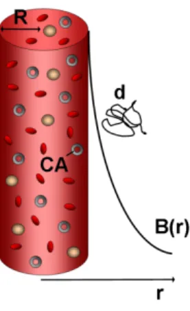
lature and the approximation of quasi static water protons. The compartmentalization of CAs, such as ultrasmall superparamagnetic nanoparticles of iron oxide (USPIO) characterized by a high magnetic susceptibility, within the randomly oriented capillary network of the brain results in localized microscopic field inhomogeneities in the tissue in which water protons diffuse, inducing a loss of transverse phase coherence with T2* signal loss in the perivascular
space. The component of the magnetic field B(r) which is parallel to B0 is inversely proportional
to the square of the distance r form the vessel B(r) ∝ ΔM (R/r)2 sin2(Θ) and it is a function of
the magnetization difference ΔM between the intra- and extravascular compartment induced by the compartmentalized CA, the vessel radius R and the angle Θ between the direction of the main magnetic field B0 and the axis of the vessel (Fig. 3). A quasi static water proton
diffusion regime assumes that the mean diffusion length of the extravascular water proton d = (D TE)½ is short with respect to the vessel radius R. In this case, the water protons situated
at different distances r from the vessel experience different magnetic field strengths B(r) and therefore diphase at different rates.
The proportionality factor between the vascular volume fraction and relaxation rate difference ΔR2* induced by the presence of the CA depends on the intra-extravascular susceptibility
difference Δχ. Monte Carlo simulations show good agreement with in vivo results [45, 53]. However Δχ has to be measured from blood samples and is sensitive to differences in hematocrit and oxygenation between the sampled blood and the microvasculature [54, 55].
Figure 3. The ΔR2* method for CBV measurement models the capillary as an infinitely long and homogeneous cylin‐
der containing the CA. The magnetic field gradient around the cylinder is a function of the cylinder radius R, of the magnetization difference between the intra- and extravascular compartment, of the cylinder orientation in the main homogeneous magnetic field B0 and of the distance from the cylinder r. The diffusion regime is said to be quasi static
when the mean water proton diffusion length d is short with respect to R, in such a way that the water protons in the vicinity of the cylinder dephase at a faster rate than those situated further away.
The CBV fraction is obtained in the following way [56]: CBV=4π3 γΔΧB1
0ΔR2 *
where γ is the gyromagnetic ratio and B0 is the static magnetic field strength.
The ratio ΔR2*/ΔR2 is dependent on the vessel size [45, 57]. ΔR2 is sensitive primarily to small
vessels, while ΔR2* is influenced by a broader range of vessel sizes. By measuring ΔR2*/ΔR2
using gradient echo and spin echo sequences, and the water diffusion coefficient D, it is possible to estimate the VSI: VSI = 0.424 (D/γΔχB0)1/2(ΔR2*/ΔR2)3/2.
5.4. Vascular space occupancy technique
The vascular space occupancy (VASO) technique [58] is a T1 weighted technique that uses an
inversion recovery sequence with timing parameters optimized to suppress the blood signal, while the extravascular tissue gives rise to a signal, which is not at its equilibrium value. For functional MRI, images are acquired during task performance (regional CBV change) and under rest conditions. It is assumed that the sum of intravascular and extravascular magnet‐ ization in a voxel is equal in the rest and in the activated condition and consequently a CBV change would inversely affect the extravascular magnetization. The signal difference between the rest and the activated condition is proportional to the CBV change. A signal decrease of about 0.7% has been detected under task performance consistent with a vasodilation [58]}. In a quantitative version of this approach [59], the absolute CBV can be determined using the T1 shortening effect of a CA. The signal before CA injection Spre is only of extravascular origin
inversion time Tinv: Spre = Sev where Sev is the extravascular signal. After CA injection, the Tinv is
sufficiently long to allow full relaxation of the blood water magnetization to thermodynamic equilibrium, and the post-contrast signal Spost is given by: Spost = Sev + S0 iv where S0 iv is the blood
signal corresponding to the thermodynamic equilibrium magnetization of the blood compart‐ ment. The signals in the difference image are proportional to the blood volume since the extravascular tissue cancels out: Spost –Spre = S0 iv.
This method is similar to the steady state T1 weighted approach except that the equilibrium
signal of the blood is acquired directly. For CBV quantification, the resulting blood signal in the difference image is normalized by the signal corresponding to the thermodynamic equilibrium magnetization of the total tissue (intra- + extravascular compartment). The normalization factor is obtained from a ROI containing cerebrospinal fluid on a reference image with sufficiently long acquisition times or from a small ROI containing mainly blood on the postcontrast image.
In humans, mean CBV of 1.4 and 5.5 ml/100 g have been measured with this technique for white matter and cortical gray matter, respectively [59].
The main difficulty encountered with this technique is that the repetition time (TR = 6 s) used is relatively long and therefore the blood T1 has to be known precisely in order to determine
the blood nulling inversion time (Tinv ≈ 1s, depending on the field strength). A slightly
inappropriate Tinv, reduced inversion efficiency or a change in blood T1 (e.g. with hematocrit
or oxygenation) results in a non negligible negative or positive blood signal before CA injection leading to a misestimation of the CBV in the difference image. Moreover, due to a relatively long Tinv, the water exchange between intra- and extravascular compartment will have a large
effect. Finally, if the normalization factor is obtained from a vascular ROI affected by a partial volume effect, the CBV might be overestimated.
5.5. The rapid steady state T1 technique
The Rapid Steady State T1 (RSST1) technique [60] is a quantitative T1 weighted MRI technique
for cerebral BVf mapping combining features of dynamic and steady state methods. Like the previously described methods it is based on a two-compartment model of the brain (intra- and extravascular) and necessitates the intravenous injection of a CA. It uses an inversion recovery (IR) prepared MRI sequence, but, in contrast to the VASO technique, a short repetition time (TR < 1 s). For such a short TR a dynamic equilibrium of the longitudinal magnetization Mz
installs in which slowly relaxing magnetization never reaches its thermodynamic equilibrium value. In addition, for tissues with T1 > 1 s, such as blood without CA and extravascular tissue,
Mz crosses the null line at almost the same inversion time Tinv (Figure 4 a). The images are
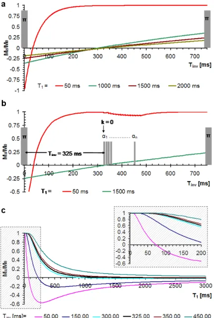
acquired using a fast low flip angle gradient echo imaging sequence FLASH [61, 62] and making sure the central k-space line is acquired when the longitudinal magnetization com‐ ponent crosses the null line (Figure 4 b). The signal evolution during this pulse sequence can be modeled [63]. Equation 4 is an approximation for the longitudinal magnetization Mz for
(
)
inv z inv 1 1 0 1 T 2exp M T ,TR,T T 1 M 1 exp TR T æ ö -ç ÷ ç ÷ è ø = -æ ö + çç- ÷÷ è ø (4)where M0 is the longitudinal magnetization at thermodynamic equilibrium and TR the
repetition time between two inversion pulses. Suppression of the longitudinal tissue magnet‐ ization can be achieved for
Tinv(TR,T1)=T1ln2−T1ln 1 + exp
(
−TRT1
)
.Figure 4 c shows Mz in function of T1 for different Tinv and TR = 750 ms.
Using a TR/Tinv couple such as 750 ms/325 ms or 500 ms/225 ms, the IR-FLASH sequence acts
like a T1 low pass filter suppressing extravascular signals having high T1 values and selectively
acquiring the intravascular signal in the presence of a CA. In particular, a blood signal at thermodynamic equilibrium is acquired when the blood T1 is below a critical value T1blood ≈
Tinv/5 after CA injection (Figure 4 a), reflecting the quantity of intravascular water protons. To
quantify the BVf, the acquired blood signal S is normalized to the thermodynamic equilibrium (proton density weighted) signal of the intra- plus extravascular tissue water S0 [60] obtained
in an acquisition with sufficiently long TR. To eliminate residual signal from extravascular compartments, such as from white matter that has lower T1, in particular at low magnetic field
strength, the average signal acquired before CA injection {Spre} is subtracted before normali‐
zation. The normalized vascular signal Snorm is then given by Snorm i=
(
Si− Spre)/
S0where S is the RSST1-signal and i denotes the time frame.
A plot of Snorm over time during and after CA injection is shown in Figure 5. For a low CA dose,
the signal time course resembles the one in Fig 2 as long as the signal is dependent on the CA concentration in blood. However, when T1blood ≤ Tinv/5 during the first pass the signal is
saturated and its amplitude equals the CBV fraction. For a higher CA dose, T1blood can be
sufficiently low for the second pass or for a longer time interval. Note that in contrast to steady state techniques, the CA concentration does not need to be in a steady state to result in a steady state signal. The name of the technique “rapid steady state” was chosen to describe the dynamic equilibrium of the signal when it becomes independent of the CA concentration, not the contrast agent concentration in blood itself.
In this way the RSST1 technique bypasses the need for conversion of the signal intensity change
into relaxation rate change and the assumption of proportionality between the latter and CA concentration. The concomitant T2 effect of the CA is minimized by using acquisitions with
Figure 4. a: The longitudinal magnetization component Mz in an IR sequence with 750 ms repetition time is plotted
after dynamic equilibrium has installed. Mz is suppressed and crosses the zero line at almost the same Tinv for tissues
with long T1, while for the same Tinv Mz is at thermodynamic equilibrium for tissues with short T1 such as blood in pres‐
ence of the CA. π = nonselective inversion pulse. b: The FLASH module acquires the image (and in particular the k = 0 line) when Mz of tissues with long T1 crosses the zero-line and blood magnetization is fully relaxed (due to the T1 short‐
ening effect of a vascular CA). Here a center-out acquisition scheme is illustrated. α = low flip angle pulse. c: Equation 4 is plotted as a function of T1 for several Tinv and TR = 750 ms. For Tinv = 325 ms Mz is suppressed for all T1 ≥ 1 s while it
Figure 5. Plot of Snorm over time. At a particular CA concentration [CA] during first and sometimes also during the sec‐
ond pass or longer, Snorm does not depend on the [CA] any more but reaches a rapid steady state (RSS) value, corre‐
sponding to the BVf.
Figure 6. a: Coronal MRI image of a mouse brain showing structural details. b: Corresponding Snorm map showing an
average cerebral BVf of 0.02 ± 0.004 and demonstrating CA accumulation in the cerebrospinal fluid leading to overes‐ timation of the CBV in periventricular structures.
The RSST1 technique was developed with CAs that remain confined to the vascular space
during the measurement such as the clinically approved small molecular size CA Gd-DOTA from Guerbet Laboraories in the presence of an intact blood brain barrier (BBB) [60]. CAs with more convenient properties are available for preclinical applications. The experimental CA P760 from Guerbet Laboratories is an intermediate molecular size CA with higher relaxivities and higher intravascular restriction (molecular weight 5.29 kDa versus 0.55 kDa, mean
diameter 2.8 nm versus 0.9 nm, longitudinal relaxivity r1 = 17.2 mM-1s-1 versus 2.9 mM-1s-1,
transverse relaxivity r2 = 27.1 mM-1s-1 versus 4.8 mM-1s-1 at 2.35 T, [64]). A rapid steady state of
at least 30 s can be obtained starting at a dose of 0.15 mmol/kg Gd-DOTA and 0.035 mmol/kg P760 at 2.35T. However, quantitative CBV maps were obtained in healthy rats with P760 at a dose of 0.1 mmol/kg and with Gd-DOTA at a dose of 0.2 to 0.3 mmol/kg. These CA doses lead to a RSS interval of up to 5 minutes that can be used for increasing the SNR, the in-plane resolution or the number of slices. Even longer RSS intervals were obtained using a continuous infusion of these CA [60]. Quantitative CBV maps were also obtained in mice at 4.7T [65]. Due to faster hemodynamics in mice and reduced relaxivities of Gd-DOTA at higher magnetic field strength, an intravenous 0.7 mmol/kg dose was used. To lengthen the RSS, the intraperitoneal administration route has been employed in mice using a 6 mmol/kg dose which was well tolerated and lead to a RSS interval of about 30 minutes starting 15 minutes after injection. Quantitatively equivalent CBV measures were obtained using the intravenous and intraperi‐ toneal routes on the same mice. A representative coronal CBV fraction map of a healthy mouse is shown in Figure 6. In studies performed repeatedly (once per month) in the same mice the cerebral BVf was well correlated between time points (Spearman r = 0.94, P-value = 0.017), with an intraindividual variability of the BVf measure in the caudate putamen of 0.018 to 0.024 (mean ± standard deviation: 0.022 ± 0.003) demonstrating the reproducibility of the CBV quantification. Intraperitoneal CA administration has the advantage of being less invasive with a lower risk for emboli and hypervolemia than intravenous administration. However, the CBV in cerebral regions close to ventricles might be overestimated due to CA arrival from the cerebrospinal fluid in which the CA accumulates.
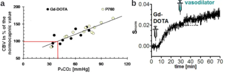
The sensitivity of the RSST1 technique to detect CBV changes has been assessed. In rats, the
measurement has been repeated under different capnia conditions [60]. Hypercapnia is induced by breathing elevated levels of carbon dioxide and results in vasodilation. In mice the vasodilator acetazolamide has been injected during the long vascular RSS interval obtained after intraperitoneal Gd-DOTA injection [65]. In both experiments, the technique has been found to be sensitive to the BVf change (Figure 7) and the degree of change was comparable with published values using different techniques [66-68].
The quantification of tumor angiogenesis is complicated by the leakiness of the vessels for these CA leading to an overestimation of the CBV in the presence of CA leakage when using
a b
Figure 7. a: A hypercapnia experiment demonstrates CBV increase in healthy rats. b: In healthy mice, the Snorm signal
a T1 weighted technique. Two strategies are possible: I) Injection of CAs that remain confined
to the vasculature despite hyperpermeable endothelium, and II) monitoring the CA accumu‐ lation in tumor tissue to be analyzed using an appropriate two compartment model.
USPIO such as AMI 227 (Sinerem, Guerbet Laboratories, Combidex, AMAG Pharmaceuticals) are widely used for their blood pool properties. They have also been used to quantify the blood volume fraction in malignant tumors in preclinical studies [69-72]. AMI 227 has a r2 relaxivity
in the order of 100 mM-1s-1 and is mainly used in T2 or T2* weighted acquisitions. The r1
relaxivity of AMI 227 (r1 = 5.4 mM-1s-1 at 2.35T) together with its blood pool property, makes it
an attractive CA for a T1 weighted technique. Sequences with ultrashort echo time (TE) need
to be used to exploit the T1 effect. Acquisition schemes starting at the center of k-space such as
radial or spiral acquisitions achieve short TE. A 3D projection reconstruction acquisition mode with a TE = 0.7 ms, was used at 2.35T to map the CBV with the RSST1 technique using 0.2 mmol/
kg AMI 227 in healthy and tumor bearing rats [73]. The post injection acquisition lasted 24 minutes, for which a steady state CA concentration in blood was assumed. The CBV meas‐ urement was compared with a steady state ΔR2* technique in the same animals (Figure 8 a).
After correction for transverse relaxation effects, both acquisition techniques yielded compa‐ rable results in healthy rat brain and a C6 glioma model. However, in a RG2 glioma model, the RSST1 technique yielded high tumor BVf while in the same ROIs the steady state ΔR2*
technique yielded BVfs that were significantly lower than in healthy or contralateral tissue (Figure 8 b). Such a discrepancy can only be explained by loss of CA compartmentalization, which results in underestimation of the BVf with T2* weighted techniques while T1 weighted
acquisitions tend to overestimate the BVf. There is also evidence for AMI 227 extravasation in the RG2 tumor model in results published by other authors [69].
In the search for intravascular CA with high r1 relaxivity for tumor BVf quantification, good
results were obtained with a novel preclinical CA based on a modified cyclodextrin [74] in a C6 tumor model [75]. This paramagnetic CA is an inclusion complex of Gd3+ with
per-(3,6-anhydro)-α-cyclodextrin. It has a molecular weight of 1464 Dalton and the shape of a flat disc. The relaxivities of Gd-ACX decrease with increased concentration, but at a 1.5 mM concen‐ tration in normal saline at 2.35T relaxivities are still r1 = 8.6 s-1mM-1 and r2 = 10.4 s-1mM-1 about
twice as high as for Gd-DOTA [64]. The biodistribution of Gd-ACX (0.05 mmol/kg) and the CBVf were studied using T1 weighted imaging and the RSST1 technique at 2.35T in healthy
and C6 tumor bearing Wistar rats 20 and 21 days after implantation, and compared to
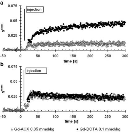
quantitative CBVf maps and the regional signal enhancement obtained after injection of Gd-DOTA. After Gd-ACX injection, the signal enhancement appears immediately in large vessels, but not in the tumor, while injection of Gd-DOTA reveals disruption of the BBB since an extensive signal enhancement is observed inside the tumor area. Representative signal versus time plots from one rat obtained by the RSST1 method in the tumor periphery and in contrala‐
teral brain tissue are shown in Fig. 9 a and b respectively. After Gd-ACX injection, Snorm remains
constant for about 5 min, while after Gd-DOTA injection the signal in tumor tissue increases continuously, reflecting CA accumulation due to a BBB leakage for this CA. Identical signal behavior in cerebral tissue contralateral to the tumor after injection of Gd-ACX and Gd-DOTA is observed (Figure 9 b). The constant signal enhancement obtained with the RSST1 technique
during the first five minutes confirms the absence of immediate Gd-ACX Extravasation from tumor vasculature allowing quantification of the tumor BVf using Gd-ACX in presence of vascular permeability to DOTA. However, the modest thermodynamic stability of Gd-ACX will limit its use to preclinical studies. For clinical applications, tumor angiogenesis needs to be assessed with clinically approved low molecular weight CA such as Gd-DOTA despite CA leakage.
Figure 9. Snorm versus time curves after Gd-ACX and Gd-DOTA injection in C6 glioma tissue (a) and contralateral brain
tissue (b). There is no evidence of Gd-ACX extravasation during the first 5 minutes after injection enabling BVf quanti‐ fication in presence of vascular endothelium permeable to Gd-DOTA.
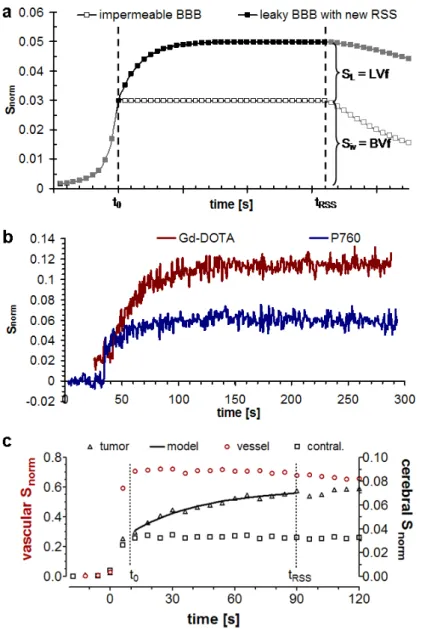
Figure 10. A model of the signal evolution during CA arrival and distribution in the tissue for two ROIs. The lower plot
represents the signal in a RSS from a ROI, in which the CA is confined to the blood pool. The upper plot displays the idealized shape of a leakage profile during the vascular RSS time window [t0, tRSS] attaining a new RSS at a signal am‐
plitude corresponding to the sum of BVf and LVf. CA = contrast agent, RSS = rapid steady state, ROI = region of inter‐ est, BVf = blood volume fraction, LVf = leakage volume fraction. b: Typical leakage profiles for a low (Gd-DOTA) and intermediate molecular size (P760) CA in a RG2 tumor model demonstrating that the vascular permeability and the total distribution volume is lower for the larger CA. c: Modeled leakage profile for Gd-DOTA in a C6 tumor model (right axis) along with RSS profiles for signal from a large vessel (left axis) and contralateral brain tissue (right axis) defining the time window [t0, tRSS] for leakage monitoring.
Unlike steady state techniques and similar to DCE-MRI, the high temporal resolution of the RSST1 technique enables monitoring of dynamic signal changes as illustrated in Figure 5.. Due
to the use of high relaxivity CA or high doses in preclinical studies, the vascular RSS is maintained over several minutes beyond the first pass. In tissues with permeable vasculature the CA extravasates leading to a continuous signal increase. If the time window for which the vascular signal corresponds to the BVf is known, the CA accumulation in tissue with permeable vasculature can be modeled. The model assumes two compartments accessible to the CA: the blood and the extravascular leakage compartment. The remaining compartments, not attained by the CA, maintain a high T1 value and do not lead to significant signal. The Snorm signal reaches
a RSS when the CA reaches a uniform concentration in the distribution compartment leading to a sufficiently low T1. As illustrated in Figure “10 a, in case of CA leakage the signal time
course approaches an asymptote. The maximum signal enhancement is then composed of the BVf and the leakage volume fraction (LVf). The Snorm signal is modeled as:
Smodel(t)=Siv+ SL
{
1−exp −κ(
t −t0)}
(5)where t0 is the beginning of the RSS time interval which can be obtained from a large vascular
structure or brain tissue with intact BBB. The BVf is estimated as Siv, i.e. Smodel in the beginning
of the signal RSS. SL is the proton density weighted signal of the extravascular leakage
compartment approximating the local extravascular distribution volume fraction (i.e. the LVf) of the CA. κ is a parameter related to the leakage rate. The CA leakage is assumed to be permeability limited [41]. Setting BVf = Siv also assumes negligible CA extravasation in the
beginning of the first pass of the CA bolus. CA backflow from the extravascular leakage compartment into the blood is not taken into account. A comparison of leakage signal profiles for two CA with different molecular weight in the same tumor tissue are shown in Figure 10 b, showing that the larger CA has a slower leakage rate and a lower distribution volume. Using Gd-DOTA, analysis of the leakage profile can therefore give valuable information about the vascular permeability which is spatially and temporally heterogenous in malignant tumors. Figure 10 c shows how the RSS time window can be determined from tissue containing impermeable vasculature in order to limit the fitting procedure to this time interval. This is not equivalent to the definition of an AIF, since the actual signal intensity is not of importance. The described methodological development of the RSST1 technique was carried out at
magnetic field strengths above 2.35T necessitating injection of high CA doses in order to compensate for the decreasing CA relaxivity with higher field strength and to achieve long vascular RSS intervals for signal averaging to overcome the low SNR in small animal imaging. In the clinical setting, the method is not only limited to Gd-DOTA-like CA, but also to low doses. In routine imaging a dose of 0.1 mmol/kg is administered, but a double or triple dose has been shown to result in higher sensitivity in particular applications. However, gadolinium based CA can result in serious complications such as nephritic systemic fibrosis in susceptible patients, it is therefore cautious to limit the administered dose to a minimum.
A pilot experiment on a 3T Philips Achieva research MRI scanner showed that CBV quantifi‐ cation with the RSST1 technique in the primate (macaque) brain is feasible with a 0.2 mmol/kg
Gd-DOTA dose at this field strength. In order to reduce the Gd-DOTA dose, the RSST1
technique has been implemented on a clinical 1.5T Philips Achieva scanner where it was integrated in the routine imaging protocol for follow up studies of neurooncological patients. The routine imaging protocol necessitated Gd-DOTA administration to look for pathological contrast enhancement on T1 weighted images, but did not include perfusion imaging techni‐
ques. A number of 120 RSST1 acquisitions (TR/Tinv = 750 ms/315 ms, matrix 64 x 55, flip angle
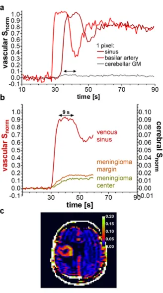
10º, inter-echo repetition time 4 ms, TE = 1.2 ms) were acquired over 90 s before, during and after CA injection using an automatic injector with an injection rate of 6 ml/s. These acquisitions were normalized to the proton density acquisition acquired before injection using the same sequence without inversion pulse and a TR of 10 s (number of averages = 3). Patients were injected with either 15 ml (= 7.5 mmol) or 30 ml (15 mmol) Gd-DOTA according to their reported or estimated weight as is often done in clinical routine, but weighted after completed examination in order to determine the administered dose precisely. In the feasibility studies, the imaging plane was chosen to include large vessels such as the basilar artery or branches of the circle of Willis and a large dural venous sinus to study the vascular signal with minimal partial volume effect. An example of the Snorm-signal profile is shown in Figure 11. It can be
observed that during the first pass of the CA Snorm reaches a value of 1 (one) corresponding to
100% blood when the voxel is placed within the vessel without partial volume effect. Conse‐ quently, the Snorm amplitude in brain tissue during the first pass reflects the CBV fraction. At
1.5T, a Gd-DOTA dose of 0.13 mmol/kg is necessary for reliable quantitative CBV fraction mapping. Below this dose, a sufficiently high CA concentration in the brain vasculature is only achieved for patients with a relatively low body mass index. The determined optimum dose is 30% higher than the recommended Gd-DOTA dose but still approved and often used in clinical practice. A RSS interval limited to the first pass of the CA has the following advantages: First, extravasation from hyperpermeable vasculature is minimized. When significant CA extravasation occurs, it can be detected as an increasing instead of a constant signal, and algorithms for leakage correction can be applied. Second, hemodynamic information can be derived. Like the mean transit time, the duration of the RSS during the first pass is related to the blood flow, but similar to first pass perfusion techniques it is also determined by the CA injection rate, dispersion and the BVf. As with first pass perfusion techniques the RSS duration relative to a reference region might still have diagnostic value.
6. What are the confounding effects?
To evaluate the accuracy of the RSST1 technique confounding effects need to be taken into
consideration. For example, the signal attenuation due to transverse relaxation has been minimized by using short TE. When T2* attenuation was significant as with AMI 227, the blood
T2* after injection has been measured to estimate and correct for this effect.
The RSST1 technique is not sensitive to blood flow effects that often affect quantification in
dynamic perfusion techniques. First, the inversion pulse is not slice selective, inverting all proton spins whether they are stationary, mobile, in the imaging plane or not. Second, when the blood T1 is sufficiently low after CA injection, the blood flowing into the imaging plane
between the excitation pulse and the readout arrives with a magnetization at thermal equili‐ brium such as the blood flowing out of the imaging plane.
However, the RSST1 technique seeks to selectively acquire signal from water molecules that
are in contact with the CA. The mobility of water molecules and their exchange across the
Figure 11. a: After an intravenous Gd-DOTA injection of 0.13 mmol/kg in patients, Snorm = 1 is attained during the first
pass in large vascular structures without partial volume effect. The Snorm amplitude in brain tissue during the first pass
(arrow) therefore corresponds to the BVf. Snorm = 0.04 in the cerebellar gray matter (GM) voxel. b: While the vascular
signal is in a RSS for about 9 s in this patient, a typical CA leakage profile is observed in the meningioma tissue. c: Snorm
map of a patient with glioblastoma. No leakage correction was applied and the BVf of 8 to 10% in the tumor border might be overestimated if significant CA leakage occurred during the first pass.
vessel wall might affect the CBV quantification. For example, water molecules that relax with a short T1 because they were in contact with the CA in the vascular compartment, but happen
to exchange to the extravascular compartment during the inversion time, will reduce the extravascular T1. This might lead to a signal contribution from the extravascular compartment
and therefore to a CBV overestimation. The RSST1 technique is based on a two compartment
model and assumes negligible water exchange between these compartments. Whether the exchange regime is fast or slow depends on the water exchange rate and on the difference between the longitudinal relaxation rates of the intravascular and extravascular compartment. An intracapillary residence time of 500 to 650 ms has been reported for healthy brain tissue [76] leading to a transendothelial exchange rate in the order of 2 s-1 which is slow compared to the
difference of the longitudinal relaxation rates between the two compartments which is in the order of 20 s-1 at the peak CA concentration. The exchange effect on the CBV measure was
evaluated using the model described in Moran and Prato [77] and showed an overestimation of 10 -12% for a Tinv of 325 ms and an assumed vascular T1 of 50 ms during the RSS. The water
exchange effect is more pronounced for higher CA agent doses or relaxivities such as used in preclinical studies. It can be reduced by shortening Tinv, allowing the compartments less time
to exchange water across the vascular boundary. For example, with the couple of parameters TR = 500 ms and Tinv = 225 ms, the overestimation would be reduced to less than 4% for a vascular T1 of 45 ms.
Strictly speaking, the blood as well as the extravascular compartment are multi compartment systems. The CA molecules do not enter the cells. However, the blood can be considered as a single compartment because even in the presence of CA molecules in plasma the intra-extracellular difference of the longitudinal relaxation rates is still one order of magnitude lower than the water exchange rate between erythrocytes and plasma (τexch-1 ≈ 125 s-1). In this fast
exchange limit, the intracellular water is affected by the presence of the CA, and it is the CBV that is measured and not the plasma volume. It is therefore not necessary to correct for the regional hematocrit.
7. How to validate a quantitative blood volume measure?
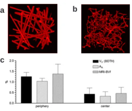
When developing new acquisition or analysis techniques the validity of their assumptions and their limits need to be assessed using reference methods ideally on the same brain. This implies either using a MRI technique that does not rely on the same principle or on the same assump‐ tions or a technique that has a different signal origin. Experimental and physiologic conditions need to be kept as similar as possible, which is not straightforward when the subject or animal needs to be moved from one scanner to another or when the measurements are a long time interval apart or relay on CAs with different properties. In particular, comparisons between in vivo and ex vivo techniques have to be interpreted with caution since the “physiologic” conditions are not alike. Nevertheless, histological validation is still the gold standard. When evaluating angiogenesis by histology, surrogate markers such as microvascular density or vascular area density are often used because they can be directly quantified from two-dimensional histological sections. The vascular volume density comes closest to the BVf but necessitates a stereological analysis of vascular morphometric data.
To validate the tumor BVf obtained with Gd-ACX by MRI, the vascular volume density was calculated as Vv = π{d}2Lv/4 where {d} is the mean vessel diameter and Lv is the vascular length
density obtained using a stereological analysis technique proposed by Adair [78]. For quanti‐ tative analysis of the microvasculature, 20 approximately equally spaced sections of 10 μm thickness were cut from the same location as the MR image (2 mm thickness). The collagen IV component of the vascular endothelium was stained using a fluorescent marker and the intravitally injected Hoechst dye was used to mark vessels which were perfused at the moment of injection. The tissue sections were digitized using a 10× magnification. ImageJ was used for segmentation and vascular morphometry. The stereological technique approximates the vessel sections as elliptical profiles of vessels modeled as randomly oriented straight cylinders. The vessel orientation was determined from the ratio of major and minor ellipse axes in order to derive Lv as described in [78]. However, no gold standard parameter exists that defines the
vessels diameter from an irregularly shaped vessel cross section. Therefore, four morphologic parameters were analyzed for their potential utility as descriptors for the vessel diameter: the radius of the inscribed circle, the minor axis of the fitted ellipses, the small side of the bounding box and the breadth. They were evaluated on a simulated idealized cylinder model and on mouse cortical vasculature obtained from two-photon microscopy data (Figure “12). Only the breadth and the minor axis of ellipse yielded reliable and physiologically appropriate diame‐ ters. These numeric data was also used to evaluate the minimum number of sections necessary to reliably quantify stereologic parameters such as the Lv. After these optimizations the
stereological analysis was applied to healthy rat brain and C6 tumor tissue and yielded vascular volume densities similar to the BVf measured by MRI with Gd-ACX. However, it was shown that only half of the tumor vessels detectable by histology were functional (perfused) vessels that contribute to the BVf measurement by MRI.
In opposite to the RG2 glioma model, the rat C6-glioma model has microvasculature permeable to Gd-DOTA but not to superparamagnetic iron-oxide nanoparticles (USPIO) allowing
a
c
b
Figure 12. Validation of the C6 tumor BVf measured with Gd-ACX and the RSST1 technique. a and b: Numerical mod‐
els used to evaluate the stereological approach: cylinder model (a) and cortical mouse vasculature (b). The stereologi‐ cal analysis of vascular morphometry confirms the tumor BVf measured by MRI (c).
validation of the BVf derived from the leakage signal time course of Gd-DOTA using a steady state ΔR2*-MRI method with an USPIO. Figure 13 a shows two BVf maps obtained with the
two MRI techniques on the same animal. Despite different spatial resolution both BVf maps reflect almost the same values and heterogeneity in the tumor. The tumor BVf and the contralateral cerebral BVf of 0.034 ± 0.005 and 0.026 ± 0.004, respectively, were confirmed, in the same rats, by ΔR2*-MRI (0.036 ± 0.003 and 0.027 ± 0.002) and also by immunohistochemical
staining (anti-collagen type IV) of perfused vessels (0.036 ± 0.003 and 0.025 ± 0.004) labeled with intravitally injected Hoechst dye. Figure 13 b shows the correlation between the three techniques.
a
b
Figure 13. Validation of the BVf obtained in a C6 tumor with the RSST1 technique by modeling the leakage signal
profile of Gd-DOTA a: Tumor BVf maps obtained with the RSST1 and a steady state ΔR2* technique with an USPIO
(MoldayION from BioPAL, Worcester, MA)as blood pool agent in the same animal show similar values and heteroge‐ neity. b: Plot demonstrating the good correlation between BVf measured with the RSST1 and the steady state ΔR2*
and with the histological vascular area density.
However, in case of USPIO leakage such as is the case in RG2 tumor tissue, the loss of CA compartmentalization reduces the magnetization difference between intra- and extravascular compartment. The CBV then tends to be underestimated with ΔR2* methods.
8. What are the quantitative values of the regional blood volume in vivo?
CBV fraction values published for healthy rats are summarized in Table 1. They are in the range of 2 to 4% with regional and technique related differences. Using the RSST1 technique
measured in healthy rats (Table 1). When using AMI 227, a lower average CBV was measured (1.6 to 2.1%) and regional differences were less pronounced probably due to the transverse relaxation effect that was insufficiently corrected for and because of a lower spatial resolution. However, steady state ΔR2* measures in the same rats confirmed the low CBV (Figure 8). In
C6 and RG2 tumor bearing rats, quantitative maps obtained with the RSST1 technique revealed
a significantly decreased contralateral CBV compared with healthy rats probably due to compression, edema, or inflammation [75], a finding also observed by other authors [71]. This shows that the vasculature in brain tissue contralateral to the tumor might not be representative of healthy brain vasculature as often assumed when reporting relative values. In a late stage C6 tumor model, a BVf of 0.98 ± 0.34% was measured in non necrotic tumor parts with the RSST1 technique and Gd-ACX, and confirmed by histology when care was taken to account for perfused vessels only.
MRI measurements in mice yield regional CBV fractions in the range of 1.7 to 2.7% including deep brain structures. Using intravital two-photon microscopy with an intravenously injected fluorescent marker, the BVf can be derived from the integrated fluorescence intensity [90]. The results in mouse brain cortex (2 to 2.4%) compare very well with the RSST1 measures, however
deeper structures are not measurable in vivo by two-photon microscopy presently limited to a depth of about 600 μm.
Figure 14.
In humans, BVf of 1.5 to 2.0% were measured in white matter, 3.5 to 4.5% in healthy appearing gray matter and values above 6% in glioblastoma margin. Figure 14 shows the BVf distribution in a healthy brain and in a glioblastoma after correction for CA leakage.
9. Conclusion
Direct quantitative mapping of the cerebral BVf is feasible with clinically approved contrast agents at a well tolerated dose during the first pass. The RSST1 technique is powerful for the
ROI CBV value unit technique reference
corpus callosum 2.0 ± 0.3% % RSST1b [60]
striatum 2.9 ± 0.6% % RSST1b [60]
cortex 3.1 ± 0.8% % RSST1b [60]
whole braina 2.51 ml/100g autoradiographyi [79]
whole braina 2.96 ± 0.57 ml/100g autoradiographyi [80]
whole brainb 2.77 ± 0.24 ml/100g autoradiographyi [81]
whole brain 1.3 ± 0.1 ml/100g autoradiographyj [82]
cortex 3.4 ml/100g optical bolus tracking [68]
whole brainc 2.40 ± 0.34 % 3D SS T 1 MRI [48] whole brainc 2.96 ± 0.82 % 3D SS T 1 MRI [83] whole brainb 3.14 ± 0.32 % SST 2-MRI [84] cortexb 1.63 ± 0.18 ml/100g SST 1-MRI [85] corpus callosumb 1.22 ± 0.25 ml/100g SST 1-MRI [85] thalamusb 3.03 ± 0.36 ml/100g SST 1-MRI [85] whole brainb 3.14 ± 0.32 % SSΔR 2*-MRI [84] cortexd 4.3 ± 0.7 % SSΔR 2*-MRI [52] striatume 3.1 ± 0.7 ml/100g SSΔR 2*-MRI [86] striatumf 2.2 ± 0.6 ml/100g SSΔR 2*-MRI [71] cortexa 3.01 ± 0.43 % SSΔR 2*-MRI [51] striatuma 2.94 ± 0.49 % SSΔR 2*-MRI [51] cortexa 4.07 % SSΔR 2*-MRI [87] striatuma 2.87 % SSΔR 2*-MRI [87]
whole brain 1.89 ± 0.39 % morphometryk [88]
whole brain without MVg 1.92 ± 0.32 ml/100g SRQCT [89]
whole brain with MVg 4.18 ± 1.06 ml/100g SRQCT [89]
cortexg 2.27 ml/100g SRQCT [89]
striatumg 2.01 ml/100g SRQCT [89]
striatumh 5.6 ml/100g SRQCT [89]
Reported values for the regional cerebral blood volume obtained with various imaging techniques. Decimal places and stand‐ ard deviations are given as reported in the original work.
ROI = region of interest, MV = macroscopic vessels, CBV = cerebral blood volume, SST1-MRI = steady state T1-weighted magnetic
resonance imaging, SSΔR2*-MRI = steady state ΔR2* magnetic resonance imaging, SRQCT = synchrotron radiation quantitative
computed tomography
arats anesthetized with halothane brats anesthetized with isoflurane
crats anesthetized with intraperitoneal pentobarbital
dcontralateral to C6 glioma, under moderate hypoxia, rats anesthetized with halothane erats anesthetized with intraperitoneal thiopental
fcontralateral to C6 glioma, rats anesthetized with intraperitoneal thiopental ganesthetized by intraperitoneal infusion of chloral hydrate
hcontralateral to F98 glioma (n = 1)
i14C-dextran labeled plasma and 99mTc labeled red blood cells j125I- labeled serum albumin and 55Fe labeled red blood cells kwith stereo correction for slice thickness, contralateral to 9L tumor
clinical practice, because it can quantify the BVf simultaneously for vasculature with or without permeability to the contrast agent, without requiring the AIF and conversion of signal intensity into CA concentration. This technique will play an important role in treatment monitoring and clinical studies in particular for the evaluation of antiangiogenic agents.
Author details
Teodora-Adriana Perles-Barbacaru* and Hana Lahrech
*Address all correspondence to: [email protected]
Grenoble Institute of Neurosciences (GIN), French National Institute of Health and Medical Research (INSERM U) – University of Joseph Fourier (UJF) – French Atomic Energy Com‐ mission (CEA) – University Hospital of Grenoble (CHU), Bâtiment Edmond J. Safra, Chemin Fortuné Ferrini, La Tronche, France
References
[1] Aronen HJ, Gazit IE, Louis DN, Buchbinder BR, Pardo FS, Weisskoff RM, et al. Cere‐ bral blood volume maps of gliomas: comparison with tumor grade and histologic findings. Radiology. 1994 Apr;191(1):41-51.
[2] Sugahara T, Korogi Y, Tomiguchi S, Shigematsu Y, Ikushima I, Kira T, et al. Postther‐ apeutic intraaxial brain tumor: the value of perfusion-sensitive contrast-enhanced MR imaging for differentiating tumor recurrence from nonneoplastic contrast-en‐ hancing tissue. AJNR Am J Neuroradiol. 2000 May;21(5):901-9.
[3] Folkman J. New perspectives in clinical oncology from angiogenesis research. Eur J Cancer. 1996 Dec;32A(14):2534-9.
[4] Zama A, Tamura M, Inoue HK. Three-dimensional observations on microvascular growth in rat glioma using a vascular casting method. J Cancer Res Clin Oncol. 1991;117(5):396-402.
[5] Folkman J. The role of angiogenesis in tumor growth. Semin Cancer Biol. 1992 Apr; 3(2):65-71.
[6] Abdulrauf SI, Edvardsen K, Ho KL, Yang XY, Rock JP, Rosenblum ML. Vascular en‐ dothelial growth factor expression and vascular density as prognostic markers of survival in patients with low-grade astrocytoma. J Neurosurg. 1998 Mar;88(3):513-20. [7] Assimakopoulou M, Sotiropoulou-Bonikou G, Maraziotis T, Papadakis N, Varakis I. Microvessel density in brain tumors. Anticancer Res. 1997 Nov-Dec;17(6D):4747-53.
![Figure 5. Plot of S norm over time. At a particular CA concentration [CA] during first and sometimes also during the sec‐](https://thumb-eu.123doks.com/thumbv2/123doknet/14216081.482729/16.722.177.549.114.475/figure-plot-norm-time-particular-ca-concentration-ca.webp)