Development and testing of three dimensional, two-fluid code THERMIT for LWR core and subchannel applications

by

J.E. Kelly and M.S. Kazimi

MIT Energy Laboratory Electric Utility Program Report No. MIT-EL 79-046

Massachusetts Institute of Technology Cambridge, Mass. 02139

DEVELOPMENT AND TESTING OF THE THREE DIMENSIONAL, TWO-FLUID CODE THERMIT FOR LWR CORE

AND SUBCHANNEL APPLICATIONS

by

J.E. Kelly and M.S. Kazimi

Report of work performed from October 1978 to September 1979

Date of Publication: December 1979

Sponsored by Boston Edison Company Consumers Power Company

Northeast Utilities Service Company Public Service Electric and Gas Company

Yankee Atomic Electric Company under

MIT Energy Laboratory Electric Utility Program Report No. MIT-EL 79-046

EXECUTIVE SUMMARY

This report describes the effort involved in the develop-ment and assessdevelop-ment of the two-fluid computer code THERMIT

for light water reactor core and subchannel analysis. The developmental effort required a reformulation of the coolant

to fuel rod coupling, found in the original THERMIT code, as well as an improvement in the fuel rod modeling capability. With these modifications, THERMIT now contains consistent

thermal-hydraulic models capable of traditional coolant-centered subchannel analysis. As such this code represents a very

useful design and transient analysis tool for LWR's.

The advantages of THERMIT are that it contains the sophis-ticated two-fluid, two-phase flow model as well as an advanced numerical solution technique. Consequently, mechanical and thermal non-equilibrium between the liquid and the vapor can be explicitly accounted for and, furthermore, no restrictions are placed on the type of flow conditions. However, the formula-tion of the two-fluid model introduces interfacial exchange

terms which have a controlling influence on the two-fluid equa-tions. Therefore, the models which represent these exchange terms must be carefully defined and assessed.

In view of the importance of these interfacial exchange

subchannel and core-wide applications. The approach followed has been to evaluate THERMIT for simple cases first and then work up to more complex flow conditions. Hence, the evaluation effort consists of performing comparison tests in the following order:

a) steady-state, one-dimensional cases, b) steady-state, three-dimensional cases, c) transient, one-dimensional cases, and d) transient, three-dimensional cases.

For these comparison tests, experimental measurements have been used when available and, otherwise,comparisons have been

made with COBRA-IV. While COBRA-IV is not as sophisticated as THERMIT, COBRA-IV is the only publicly available subchannel code capable of analyzing reverse flow conditions.

As a result of these comparisons, the following conclusions can be made. First, it is found that THERMIT can adequately predict the void fraction for a wide range of flow conditions.

This result implies that both the subcooled vapor generation

model and the interfacial momentum exchange model are appropriate. A second conclusion is that, while the heat transfer

model is generally appropriate, specific parts of this model may need to be improved. For example, the calculated critical heat flux is consistently too low. Hence, some improvement can be made in the prediction of the CHF location. However, the pre-CHF wall temperatures are satisfactorily predicted and do not require improvement. The post-CHF temperatures are also adequately predicted even though there are some

differences are not uncommon for the post-CHF regime since the data base for the heat transfer correlations is limited. Nevertheless, some of these differences may be due to the

method in which the heat transfer model is coupled to the fluid dynamic solution. Consequently, this coupling needs to be

evaluated to insure that it is appropriate.

A third conclusion is that in order to accurately predict the flow and enthalpy distribution in subchannel geometry,

a turbulent mixing model must be added to THERMIT. Both single-phase and two-single-phase measurements illustrate this point. Without such a model, the mass flux and quality predictions are poorly predicted.

In addition to the above mentioned validation efforts, the core-wide and transient capabilities have also been assessed. From these comparisons it can be concluded that, on a core-wide basis, THERMIT can accurately predict the core exit temperature distribution. This conclusion is based on comparisons with both measurements and COBRA-IV predictions.

It has also been found that THERJ4IT can accurately predict one-dimensional blowdown transients. For transients of this

type, the wall friction and vapor generation rate have the greatest effect on the code predictions.

Finally, for multidimensional transients it can be concluded that the predictions of THERMIT appear to be qualitatively

correct and, additionally, THERMIT is at least as computationally efficient as COBRA-IV (explicit). Differences between the

predictions of the two codes may be anticipated in light of their respective two-phase flow models.

TABLE OF CONTENTS Page EXECUTIVE SUMMARY ... ... ... . 1 TABLE OF CONTENTS ... 4 LIST OF FIGURES ... ... 6 LIST OF TABLES ... 8 NOMENCLATURE ... ... 9 Chapter 1. INTRODUCTION ... 11

Chapter 2. THERMIT DEVELOPMENT ... 17

2.1 Introduction ... 17

2.2 The Two-Fluid Model and Solution ... 17

2.2.1 Two-Fluid Model ... 17

2.2.2 Solution Procedure ... 20

2.2.3 Capabilities of Initial Version of THERMIT ... 21

2.3 Subchannel Version ... 22

2.3.1 Coolant Centered Channels ... 23

2.3.2 Fuel Rod Modeling ... 24

2.4 Other Code Improvements ... 25

2.4.1 Vapor Generation Model ... 25

2.4.2 Interfacial Momentum Exchange Model ... 28

2.4.3 CHF Correlation ... ... 28

Chapter 3.

Chapter 4.

VALIDATION AND ASSESSMENT OF THERMIT ... 3.1 Introduction ... ... 3.2 Steady-State, One Dimensional Comparisons

3.2.1 Void Fraction Comparisons ... 3.2.2 Clad Temperature Comparisons ... 3.3 Steady-State, Three-dimensional

Comparisons ... 3.3.1 Isothermal Subchannel

3.3.2 Heated Subchannel Data ... 3.3.3 Core Exit Temperature Measurements 3.4 Transient One-Dimensional Comparisons ... 3.5 Transient Multidimensional Comparisons .. 3.5.1 Rod Ejection Accident ... 3.5.2 Hot Zero Power Initial Condition

Case ... 3.5.3 Low Flow, Low Power Initial

Condition Case ... DIRECTIONS FOR FURTHER DEVELOPMENT ...

APPENDIX A - DESCRIPTION OF THE SUBCOOLED VAPOR GENERATION MODEL ... ... 104 MODEL.*-e---*---@---@---@---- 104 APPENDIX B - DESCRIPTION OF INTERFACIAL MOMENTUM

EXCHANGE MODELS ... ... 110 APPENDIX C - DESCRIPTION OF CHF CORRELATIONS ... 116 APPENDIX D - THERMIT COMPARISONS WITH STEADY-STATE,

ONE-DIMENSIONAL DATA ... 121 ACKNOWLEDGEMENTS ... .... 1535...3... 34 34 37 37 57 65 65 71 76 78 85 85 88 91 99

LIST OF FIGURES

FIGURE No TITLE PAGE

2.1 Comparison of Void Fraction Profiles ... 27 3.1 Typical Void Fraction versus Enthalpy Data ... 42 3.2 Void Fraction versus Enthalpy - Maurer Case 214-3-5 ... 45 3.3 Void Fraction versus Enthalpy - Christensen Case 12 ... ... 47 3.4 Void Fraction versus Enthalpy - Christensen Case 13 ... 48 3.5 Void Fraction versus Enthalpy - Composite of

Christensen Cases 12 and 13 ... 49 3.6 Void Fraction versus Enthalpy - Marchaterre Case 168 ... 51 3.7 Void Fraction versus Enthalpy - Marchaterre Case 184 .... 52 3.8 Void Fraction versus Enthalpy - Christensen Case 12 ... 54

3.9 Vapor Superficial Velocity versus Void Fraction for

Christensen Data ... 55 3.10 Vapor Superficial Velocity versus Void Fraction

-Comparison of Data with THERMIT ... 56 3.11 Typical Wall Temperature versus Axial Height Curve ... 61 3.12 Wall Temperature versus Axial Height - Bennett

Case 5394 ... ... ... 62 3.13 Wall Temperature versus Axial Height - Bennett

Case 5273 ... ... 64 3.14 Schematic Drawing of 9 Rod Bundle Cross Section ... 66 3.15 Radial Peaking Factors for Non-Uniformly Heated Case ... 72 3.16 Measured versus Predicted Coolant Temperature Rises

-Maine Yankee 1/8 Core Analysis ... 77 3.17 Comparison of THERMIT and COBRA-IV Exit Temperature

FIGURE No TITLE PAGE

3.18 Schematic Drawing of Edwards' Blowdown Pipe ... 81 3.19 Pressure-Time Histories for Edwards Pipe Blowdown Test.. 83-84 3.20 Normalized Transient Power Distribution Used in Rod

Ejection Accident Cases ... ... ... 86 3.21 Clad Temperature versus Time-Rod Ejection Accident

from HZP Condition ... . 89... 89 3.22 Void Fraction versus Time-Rod Ejection Accident

from HZP Condition ... . ... ... 90 3.23 THERMIT Space-Time Void Fraction Distribution-Rod

Ejection Accident from Low Flow, Low Power Condition ... 93 3.24 COBRA-IV Space-Time Void Fraction Distribution-Rod

Ejection Accident from Low Flow, Low Power Condition ... 94 3.25 THERMIT Inlet and Outlet Mass Flux Distributions versus

Time-Rod Ejection Accident from Low Flow, Low Power

Condition ... 95 3.26 COBRA-IV Inlet and Outlet Mass Flux Distributions versus

Time-Rod Ejection Accident from Low Flow, Low Power

Condition .. ... ... ... 96 3.27 Clad Temperature versus Time-Rod Ejection Accident from

TABLE No 1.1 1.2 2.1 3.1 3.2 LIST OF TABLES TITLE

THERMIT Advantages over COBRA-IIIC/MIT .... THERMIT Advantages over COBRA-IV ...

Summary of Remedies Used to Reduce CPU

Requirements for Steady-State Solutions ...

Summary of Evaluation Procedure ... Test Conditions for One-Dimension Steady-State Data ... Summary of Heat Transfer Regimes ... Single-Phase Data Comparisons for GE 9 Rod Bundle ... Initial Conditions for Rod Ejection

Transients ... 3.3 3.4 3.5 PAGE 14 15 31 38 44 59 70 87

NOMENCLATURE A Area Cp Specific heat D_h Hydraulic Diameter e Internal Energy f Friction Factor F Gravitational Force

F_i Vapor-Liquid Interfacial Momentum Exchange Rate F Wall Frictional Force

w

g Gravitational Constant

G Mass Flux

h Enthalpy

H Heat Transfer Coefficient Jv Superficial Vapor Velocity k Thermal Conductivity

Ki Interfacial Momentum Exchange Coefficient

L Length

N Bubble Number Density

P Pressure

Q. Interfacial Heat Transfer Rate Qw Wall Heat Transfer Rate

q Power

Re Reynolds Number

Sij Gap Spacing Between Coolant Channels

t Time

T Temperature

T_d Bubble Departure Temperature Ts Saturation Temperature

V Velocity

VR Relative Velocity w!. Turbulent Mixing Rate

13

X Quality

a Void Fraction Mixing Parameter

r

p Density

1P- Viscosity

SUBSCRIPTS

i,j,k Nodal Locations

z Liquid

s Saturation

v Vapor

1. INTRODUCTION

In the last few years, the need for improved assessment of nuclear reactor safety has lead to the rapid development of methods for multidimensional two-phase thermal-hydraulic analysis. These methods have become progressively more complex in order to account for the many physical phenomena encountered in two-phase flow. These phenomena include non-equilibrium conditions between the vapor and the liquid such as subcooled liquid boiling, vapor condensation and relative motion of the two phases. Furthermore, elaborate solution methods have been used so that the complex flow patterns encountered in postulated transients may be analyzed. For example, in a loss of coolant accident (LOCA) or a severe anticipated transient without scram

(ATWS), flow reversal may occur and the numerical method must be capable of handling such a condition. Hence, these new multidimensional thermal-hydraulic computer codes combine

complex physical modeling with advanced numerical solution techniques.

The MIT developed computer code, THERMIT (1), is an example of these advanced codes. THERMIT solves the three-dimensional, two-fluid equations describing the two-phase flow and heat transfer dynamics of light water reactor cores in rectangular coordinates. The two-fluid equations describe the

A complete set of conservation equations is written for each phase, accounting for the interactions between the phases. These equations are very general and are only limited by the choice of the interaction terms. Hence, both BWR and PWR cores can be modeled and analyzed under steady-state as well as

transient conditions.

The two-fluid equations are solved in first-order finite difference form with a semi-implicit solution technique. This technique is a modified version of the ICE method (2,3) and has a stability restriction in the form of a maximum allowable time step:

At < AX/V (1.1)

where AX is the mesh size and V is the larger of the vapor and liquid velocities. At each time step, the equations are solved with a Newton iteration method which reduces the system of equations to simplified boundary value problem for pressures only. A unique feature of this method is that convergence can always be obtained if small enough time steps are chosen.

Consequently, this solution is ideally suited for severe transient analysis.

Although originally developed as a tool for core-wide analysis, THERMIT is flexible enough to be adapted to analyze other types of two-phase flow conditions. One useful extension would be to modify the code so that it is capable of subchannel

analysis. Such a tool would have several advantages over widely used codes such as COBRA IIIC/MIT (4) or COBRA IV (5). For analyses of two-phase conditions, compared to COBRA IIIC/MIT

THERMIT has the advantages listed in Table 1.1. It is seen that both the improved physical model and the numerical

method lead to significant improvements. Similarily, a sub-channel version of THERMIT would also have advantages over

COBRA IV as summarized in Table 1.2. Again the improved physical model and numerical method lead to improvements although not

as many as in the COBRA IIIC/MIT case.

In view of these advantages, the development of a sub-channel version of THERMIT has been undertaken. The purpose of this effort is to provide the utilities with an advanced tool capable of both core-wide and subchannel thermal-hydraulic analysis. With such a tool, it is now possible to analyze

problems which could not have been analyzed using less advanced methods. Furthermore, it is also possible to assess the appli-cability of these less sophisticated methods. Hence, the

development of a subchannel version of THERMIT represents a significant advancement in core thermal-hydraulic analysis. The strategy for developing the subchannel version of THERMIT has been to

a) modify the code structure and numerical method as necessary,

b) verify and assess existing models for physical phenomena and

Table 1.1 THERMIT Advantages over COBRA-IIIC/MIT

A. Permanent Advantages of the Physical Model and Numerical Method

1. True 3-D flow equations, i.e., no approximation in transverse momentum equation

2. The two-phase flow model allows:

a) Unequal temperatures for each phase b) Superheated vapor

c) Compressibility effects

d) Countercurrent or cocurrent flow of the two phases

3. The numerical method allows: a) Flow reversals

b) Pressure boundary conditions c) Guaranteed convergence

B. Current Advantages

1. Improved heat transfer model which includes:

a) Complete boiling curve heat transfer calculations b) Advanced gap conductance model

c) Temperature dependent fuel properties d) Fully-implicit clad-coolant coupling

(COBRA-IIIC/MIT is being upgraded to compensate for these advantages)

Table 1.2 THERMIT Advantages over COBRA-IV

1. True 3-D flow equations, i.e., no approximation in transverse momentum equation

2. The two-phase flow model allows:

a) Unequal velocities for each phase (explicit version only)

b) Unequal temperatures for each phase

c) Subcooled liquid boiling (explicit version only) d) Compressibility effects

e) Countercurrent or cocurrent flow of the two phases 3. Improved heat transfer modeling which includes:

a) Advanced gap conductance model

b) Temperature dependent fuel properties 4. More advanced numerical method which allows:

a) Guaranteed convergence

b) Flow reversals (implicit version only)

Modifications, such as providing the capability to analyze coolant centered subchannels, are discussed in Chapter 2. Improvements which have been implemented in THERMIT are also discussed in Chapter 2. The verification and assessment of the models in THERMIT are discussed in Chapter 3.

2. THERMIT DEVELOPMENT

2.1 Introduction

In this section the effort to develop the capability for subchannel representation and the modification of the

models provided in THERMIT are described. The original THERMIT code structure and models are detailed in Reference 1. It is assumed here that only the changes from that structure need be discussed in detail. A brief account of the original THERMIT formulation will be given also.

2.2 The Two-Fluid Model and Solution 2.2.1 Two-Fluid Model

The two-fluid model in THERMIT treats each phase (either liquid or vapor) as a separate fluid which results in the following conservation equations:

Conservation of Vapor Mass: (2.1)

at (apv ) + V- (ap Vv) = r

Conservation of Liquid Mass:

t [ ( 1 - _{) pi] + V. [(1- a)pVp] = -r}

Conservation of Vapor Energy:

a (p ) aew)Pv4. at

at

(aPvev)

(2.2)

Conservation of Liquid Energy: (2.4)

a

aa

at

)p

= Qw - Qi

Conservation of Vapor Momentum:

av 5

ap v + pv(Vv. V)VV+ aVP = -FW -F - pg (2.5)

Conservation of Liquid Momentum:

(1 - a) P at + (- a) (V V)V+ (1- a)VP = -Fw +F i (2.6)

-(1- a) P g

(See Nomenclature Table on page 9 .)

In addition to these conservation equations there are four equations of state, i.e.

Pv = Pv(P, Tv) (2.7)

pk = pt(P, T) (2.8)

e_v = ev(P, T_v) (2.9)

e = e (P, T) (2.10)

In total then there are ten conservation equations (2 mass, 2 energy, 6 momentum) and four equations of state or fourteen total equations. The fourteen corresponding unknowns are the void fraction, a, the pressure, P, the densities, v and pk, the internal energies, ev and e, the temperatures, T_v

and T, and finally the three components of the velocity vectors, Vv and V. It is clear therefore that the liquid and vapor pressures within any control volume are assumed equal.

This two-fluid formulation of the conservation equations introduces terms that represent interactions within any given control volume. These interactions can be classified as

being either vapor - liquid or fluid-wall interactions. The vapor-liquid interaction terms are the vapor production rate

(or the mass exchange rate),

r,

the phase boundary. The fluid-wall interaction terms are the wall heat transfer, Qw' and the wall friction loss, Fw_. Each of these processes represent a transfer mechansim between

either the liquid or vapor and the structural material (e.g. fuel rods, grids). Models for each of these interaction

terms, usually referred to as the constitutive equations, are required to close the system of equations. These models are empirically or semi-empirically based. Due to the precise physical interpretation of these terms, the models should be valid over a wide range of conditions.

Hence, it is seen that the two-fluid model is rather complex. Nevertheless, the model is not restricted by assumptions such as the homogeneous equilibrium assumption

4. 4.

(V= = Vv, T = Tv = T ) Therefore, the two-fluid model is well-suited for severe transient analysis, where non-equilibrium

effects may be significant. 2.2.2 Solution Procedure

The above set of equations is solved with a semi-implicit numerical method as discussed in Reference 1. This method can be outlined as follows. The conservation equations are first approximated by a linearized set of finite difference

equations. The density and internal energy in these equations are then eliminated in favor of the pressure and temperatures by using the equations of state. The momentum equations are then used to derive a relationship between velocity and

pressure which can be used to eliminate the velocity in the mass and energy equations. The resulting system of

equations for each node can be represented as follows:

+ 1 x x x P x x x x P x X X o X X XXXX P+1 X x +x x x x(2.11)x x XXX jlP-1 x x x x Tk x x x k+l x Pk-l

where each x represents a known coefficient. One notes that these equations couple together the pressure in the node, the void fraction, the liquid and vapor temperatures and the pressures in the six adjacent cells. By multiplying through by the inverse of the 4x 4 matrix, the only unknowns in the first equation that remain are the pressures. This equation

is solved iteratively for every node with each sweep through the core referred to as an inner iteration. Once the pressure

distribution is found, the other unknowns (a, Tv, T) can be found by back substitution. The inversion of the 4x 4 matrix and subsequent back substitution is referred to as a Newton or outer iteration.

This method converges on the pressure distribution with the user controlling the convergence criteria and the number of iterations (both inner and Newton). If convergence is not attained in the specified number of iterations, the code has the capability of reducing the time step size. The

advantage of this feature is that if the time step size is small enough, the method will always converge. Hence, this solution method is extremely reliable for any type of flow conditions.

2.2.3 Capabilities of Initial Version of THERMIT

The numerical method in THERMIT was originally developed for core-wide analysis. In other words, transients which could be analyzed using a coarse mesh (i.e., assembly-sized control volumes) would be well-suited for THERMIT. Consequently, the initial developmental effort at M.I.T., which was sponsored by EPRI, focused on the idea of using assembly-sized control

vol-umes in THERMIT. The thrust of our current effort is to demon-strate that analyses with subchannel sizes can also be handled by the basic scheme.

With large control volumes, certain practical simplifica-tions can be made. For example, since only the average fluid conditions are calculated in each assembly, only one average

simplifies the coupling between the coolant and fuel rod. Additionally, the effects of turbulent mixing should be small and the above effects may be neglected. Hence, it is seen that the use of assembly-sized control volumes can lead to some modeling simplifications.

In view of this type of application for THERMIT, the various constitutive models were tuned for use with large control volumes. For example, the interfacial friction model was developed using BWR bundle average void fraction data. Modeling of the transverse wall friction was also based on

assembly-size volumes, since the friction correlation was developed for flow normal to an infinite rod array.

2.3 Subchannel Version

For a large number of applications, details of the two-phase within an assembly are of interest. Although a coarse mesh core modeling had originally been envisioned when using THERMIT, there is no intrinsic reason to limit the code

appli-cability to small mesh sizes. From a numerical point of view, the solution method would not explicitly restrict the size of the mesh. However, due to stability considerations, a mesh size smaller than 2 x 10-4m may lead to problems (6). This limit is at least 30 times smaller than subchannel size. The primary limitation on the applicability of THERMIT regarding

subchannel applications was that the constitutive models may not have been applicable for these applications. In particular, the lack of a turbulent mixing model and the infinite-array

transverse friction model were significantly inappropriate. Another shortcoming was that only one fuel rod per channel could be

modeled. Consequently, the traditional coolant centered subchannel, in which four fuel rods (actually quarters of fuel rods) and the gaps between them make up the boundaries of the subchannel,

could not be modeled.

In order to overcome these restrictions, a code development effort has been undertaken. This effort has been directed at improving THEPR4IT by developing a subchannel version and

evaluating the code's predictive capabilities. The specific modifications to THERMIT are discussed below.

2.3.1 Coolant Centered Channels

The first step in this development was to modifiy the code so that coolant centered subchannels could be modeled. This process involved changing all the coupling between the clad and coolant temperatures. This coupling occurs in the energy equations as outlined in Reference 1. These equations were changed so that each coolant channel could be coupled to

a maximum of four fuel rods. Hence, the source term in the energy equations would become a sum of up to four terms, one from each adjacent rod.

Changes were also required in the wall friction selection logic. As originally programmed in THERMIT, the partitioning of the wall friction would be as follows:

F = 0

wv } if T < T (2.12)

F = F CHF

F =0 if T > Tmsfb (2.13) F F wv wT F = qv F wv - wT q" + q" v } if TCH_F<T <Tmsfb (2.14) Fw~Z - FwT CHF w msfb Fwk qk FwT qQ + qv

This logic is dependent on the clad temperature or more

appropriately the wetting characteristics of the clad. With the potential of four heated surfaces in a channel, it became necessary to define which clad temperature should be used in this logic. A search routine was added to determine the maximum clad temperature in each coolant node and this value would be used in the wall friction selection logic.

2.3.2 Fuel Rod Modeling

Along with applications involving coolant centered

subchannels came the need to have detailed fuel rod modeling. In practical terms this meant having the ability to calculate four clad temperatures per fuel rod. With this capability, the fuel rod modeling would be consistent with the clad-coolant coupling.

This was accomplished by allowing each quarter of a fuel rod to be modeled separately. Hence, it would be possible to have four clad temperatures per fuel rod. In fact, a complete heat transfer calculation is performed for each rod section

(whether it be a quarter, half or full rod) so that the temperatures throughout the section are calculated.

Consequently, for any given rod modeled as four sections, there will be four centerline temperatures calculated which are not necessarily equal. This may not always be accurate due to azimuthal heat conduction effects which are neglected here. For cases of practical importance which have been run, negligible differences in the centerline temperatures were calculated. Another minor disadvantage of this method is that the computational time will be increased, but this increase should not be excessive. Therefore, on the whole, the fuel pin modeling together with the coolant-centered subchannel capabilities provide THERMIT with the geometrical flexibility required for subchannel analysis.

2.4 Other Code Improvements

A number of other improvements in the overall THERMIT model have been implemented. Some of these improvements modify the original constitutive models which are described

in Reference 1. The models affected are the vapor generation model, F, the interfacial momentum exchange model, Fi, and

the critical heat flux model. Other improvements have been added to reduce the computational effort required to obtain a steady-state solution. Each of these improvements is discussed below.

2.4.1 Vapor Generation Model

In the original version of THERMIT, only one vapor generation model had been available; namely the Nigmatulin model. Since its initial release, a second option has been

added to THERMIT. This model has been termed the subcooled boiling model because it allows vapor generation even for subcooled fluid conditions. Consequently, subcooled boiling can now be predicted, which was not the case in the original

version.

The formulation of this model is based on the work of Ahmad [7]. In this model it is assumed that the heat flux

to the coolant can be divided into two parts. One part raises the liquid temperature and the other part generates vapor. A prescription is then given for the fraction of the heat

flux used to generate vapor. Then using a simple heat balance and a condensation model based on non-equilibrium effects

the vapor generation model is obtained. The details of this model are given in Appendix A.

To illustrate the advantages of this new model a comparison between this model and the Nigmatulin model has been performed. In this test case, a BWR bundle has been modeled as a single channel and a void fraction versus axial length comparison has been made. As seen in Figure 2.1, over the last 60% of the channel the two models are in good agreement which simply indicates that both predict the same vapor generation rate in saturated boiling conditions. However, in the subcooled

boiling regime (first 40% of the channel) there is a sub-stantial difference in the vapor generation rate and,

consequently, the void fractions differ. With the subcooled boiling model, boiling is predicted to occur earlier in the channel. The void fraction differences are significant for

.7 .6 .5' z 0 H I/ E-1 H :> 3 .2 o/ Ca

Figure 2.1 Comparison of Void Fraction Profiles.

o .25 . .75 4o

reactivity considerations and, hence, the subcooled boiling model would yield the more realistic results for BWR and PWR cases.

2.4.2 Interfacial Momentum Exchange Model

The interfacial momentum exchange model provided in the original THERMIT did not prove to be very accurate and has been replaced. In fact, two models were added which give more realistic results. The first model was developed by Stewart [8] at M.I.T. and the second one is used in the two-fluid models at LASL [9]. Each of these models has been used in void fraction comparisons which are discussed in Section 3.2.1. The details of each model are given in Appendix B.

2.4.3 CHF Correlation

The original version of THERMIT contained only one CHF correlation. This correlation, namely the Biasi correlation, is part of the BEEST heat transfer package 0] which has been developed for blowdown heat transfer analysis. The selection of the Biasi correlation for blowdown applications is based primarily on its data base, which covers a wide range of pressures and includes both upflow and downflow conditions. Essentially, this correlation is a "dry-out" type CHF

correlation which is consistent with the expected CHF type during blowdown. However, for DNB type CHF or for non-uniform axial power distributions, the Biasi correlation would not be applicable. Therefore, in view of these shortcomings, additional CHF correlations have been added to THER4IT.

The two correlations selected to complement the Biasi correlation are the W-3 correlation and the CISE correlation. Each of these correlations can be found in the open literature and are reproduced in Appendix C. The W-3 correlation can be used for steady-state and transient PWR conditions while the CISE correlation can be used for similar problems in BWR systems. Together with the Biasi correlation, these correlations should cover the range of practical interest.

2.4.4 Steady-State Options

Although the semi-implicit solution method in THERMIT is well-suited for transient analysis, there is no convenient way to obtain steady-state solutions with this method. The

reason for this is that some of the temporal finite difference equations are written explicitly and, hence, the maximum

permissible time step size is limited by the Courant velocity condition (i.e. At < Ax/v). Consequently, an infinite value for At cannot be used as one would like to use for steady-state problems (i.e. 1/At = 0). Instead, steady-state solutions are found by starting from an initial guess and then running an

unperturbed transient until an equilibrium solution is achieved. This equilibrium solution is the steady-state solution from

which a true transient may be initiated.

This method of finding steady-state solutions by solving an initial value problem cannot be changed except by going to a fully implicit method. Therefore, techniques for improving the computational efficiency of this method have been

take advantage of the presumed nature of the steady-state

solution. For example, the fuel rod heat flux in steady-state must equal the linear power rate divided by the heated

perimeter. Therefore, there is no need to solve for the heat transfer coefficients and clad temperatures until the fluid dynamics have converged. In other words, the heat transfer calculations are initially eliminated. Basically, this technique decouples the heat source from the coolant which can lead to substantial CPU savings (See Table 2.1).

Another technique which has been developed to increase the computational efficiency of finding steady-state solutions is called the isolated channel method. It takes advantage of two features of the steady-state solution procedure and one physically based assumption. The first feature of the

solution procedure is that one-dimensional problems converge much quicker than do three-dimensional problems. For example,

four isolated channel require less CPU time to reach steady-state than do four connected channels. A second feature is that the closer the initial conditions are to the steady-state, the quicker the method will converge. This means that if one can improve the selection of the initial conditions, then a

steady-state solution may be obtained with less computational effort. The physical assumption is that in most cases the transverse flow between channels is small. This assumption means that the pressure and flow distributions can be

approximately determined by treating the channels as though they were isolated. Hence, a good initial guess can be

TABLE 2.1

SUMMARY OF REMEDIES USED TO REDUCE

CPU REQUIREMENTS FOR STEADY-STATE SOLUTIONS

Remedy Reduction of CPU

Isolated Channel Method+ 25 - 90%

Elimination of Heat Transfer Calculation 10 - 25%

Double Precision* 7%

The isolated channel case essentially provides a good guess of the flow and pressure fields. This remedy will work as long as the transverse flow is small so

that the radial pressure distribution is not signifi-cantly altered when the gaps between channels are assumed open.

This remedy was tested and showed limited improvement, but due to the increase in core storage it has not been implemented.

obtained using the calculational results of the isolated channel problem which require very little computational effort. Then, once this solution is obtained, the interconnecting gaps can be opened to allow the appropriate flow redistribution to occur. The unperturbed transient is then continued until a true

steady-state is reached. As seen in Table 2.1, this method leads to a substantial reduction of the CPU time. It should be noted that this technique may not be as beneficial in cases where large inter-channel crossflows are expected in steady-state, since the isolated channel case would no longer represent a good initial guess.

Both the option to eliminate the heat transfer calcula-tions (i.e., use a constant heat flux boundary condition) and the option to use the isolated channel method have been imple-mented into THERMIT. The use of either option is controlled by

an input flag. The input flag iqa controls the type of heat transfer boundary condition:

= 0 constant heat flux

4s . = Inormal

The input flag itam controls the use of the isolated channel method:

= O isolated channel method itam

= 1 normal

Both of these input flags must be specified by the user and can be changed with the restart option. Hence, a steady-state

would be obtained by initially running an unperturbed transient with iqas = 0 and itam = 0 for a specified length of time

(typically 2.0 seconds). The problem would then be restarted with iqa = 1 and itam = 1 and the unperturbed transient would be continued until steady-state is reached (typically an additional 2-3 seconds). Using this technique the computational efficiency of finding steady-state solutions is greatly increased.

3. VALIDATION AND ASSESSMENT OF THERMIT

3.1 Introduction

In conjunction with the developmental effort discussed in Chapter 2 a program for validating and assessing the models in THERMIT has been undertaken. The goals of this program are:

(1) To validate the predictive capabilities of THERMIT and (2) To define the needed models and assist in developing them. The emphasis in this effort has been directed toward evaluating

the code for subchannel applications. In particular, the following models and capabilities have been investigated:

a) r, the vapor generation rate model,

b) Fi, the interfacial momentum exchange rate model,

c) Qw' the wall heat transfer rate model, and d) The three dimensional flow modeling.

In addition to developing and verifying a subchannel version of THERMIT, the original version of THERMIT has also been assessed.

In order to meet the goals of this program, an orderly progression of tests and comparisons has been performed.

These include comparisons with both one-dimensional and three-dimensional experimental data and multidimension comparisons with other computer codes (e.g., COBRA IV). The order in which these comparisons have been made is structured so that individual models can be validated and assessed in a logical manner. This procedure entails first selecting a set of

experimental data which can be used to validate a specific model independent of the other models in the code. Once a model has been validated, it can be used with some confidence in the effort to validate the other models. For cases in which experimental data are not available, comparisons can be made with other computer codes. In this way, the data base for

the code is built-up in a systematic manner.

Experimental measurements suitable for model evaluation need to be simple so that individual models can be validated without introducing extraneous effects. Consequently,

steady-state, one dimensional measurements serve as a logical starting point for the validation program. Measurements of this type do not contain any temporal or multi-dimensional effects and

the conservation equations can be greatly simplified. The next step in complexity would be isothermal, steady-state, three dimensional tests. In measurements of this type, there is no heat transfer so that the energy equation can be elimi-nated. Next, steady-state, heated, three-dimensional experiments can be used. Measurements of this type have additional

com-plexities and, hence, it is imperative that the simpler cases are evaluated first. Finally, after completing these steady-state evaluations, both one-dimensional and multi-dimensional transient conditions would be investigated.

In this systematic procedure, the initial evaluation has been performed using steady-state, one-dimensional void

both the vapor production rate, r, and the interfacial momen-tum exchange rate, F.. A large number of data sets have been compared with THERMIT and these comparisons are discussed in section 3.2.1.

The second type of data used in this effort is steady-state, one-dimensional heat transfer data. This data is in the form of clad temperature distributions and is useful for evaluating the heat transfer model. Comparisons between the data and THERMIT predictions have been performed and are discussed in section 3.2.2.

Steady-state, three-dimensional measurements have also been used. Measurements for both isothermal and heated sub-channel experiments have been compared with THERMIT. A

discussion of these comparisons can be found in sections 3.3.1. and 3.3.2. Measurements of the core exit temperature

dis-tributions have also been compared with THERMIT. These comparisons require using the core-wide modeling approach and are discussed in section 3.3.3.

The first transient case which has been compared to THERMIT is a one-dimensional blowdown application. Experi-mental measurements for this case have been used to assess the ability of THERMIT to analyze a very severe transient. The results of this comparison are discussed in section 3.4.

The final case, which has been used in this evaluation program, is a two-dimensional simulation of a rod ejection accident (REA). For this case, THERMIT has been compared to

COBRA-IV in order to assess the transient capabilities of

THERMIT. Two different REA's are considered in this analysis. The first REA is initiated from a hot zero power condition while the other REA is initiated from a low flow, low power condition. The comparisons for these cases are discussed in section 3.5.

This evaluation program is summarized in Table 3.1. These tests do not cover all possible conditions of interest and futher testing is required. However, this evaluation program establishes a reasonable format for future investi-gations.

3.2 Steady-State, One Dimensional Comparisons 3.2.1 Void Fraction Comparisons

The ability to accurately predict the void fraction distribution is of major importance for both reactor safety and design purposes. Hence, it is essential that THERMIT be able to predict the void fraction distribution. However, in THERMIT there is no correlation for the void fraction as is found in other codes (e.g., COBRA IV). Instead, the void

fraction is a variable in the solution method and is controlled by a combination of the vapor generation rate and the interfacial

momentum exchange rate. Hence, the void fraction will depend on the selection of these two models.

The way in which these models affect the void fraction can be explained by considering each model separately. The vapor generation rate model must account for two types of

TABLE 3.1

SUMMARY OF EVALUATION PROCEDURE

1. Steady-State A. Void B. Clad One Dimensional Fraction Temperatures

2. Steady-State Three Dimensional A. Unheated Subchannel Data

B. Heated Subchannel Data

C. Core Wide Temperature Distribution

3. Transient One-Dimensional

A. Blowdown Transient Data 4. Transient Multi-Dimensional

A. Simulated Rod Ejection Accident

1) Hot Zero Power Initial Condition

boiling conditions; namely subcooled boiling and saturated boiling. In the subcooled boiling regime, this model must predict the location where boiling begins as well as the amount of vapor being generated. In the present model, the Ahmad correlation is used to determine the bubble departure

location and non-equilibrium effects are accounted for in the subcooled vapor generation rate (11). In the saturated

boiling regime, the model reduces to an equilibrium model in which all the heat added to the channel results in vapor production, i.e.,

r = q/hfg (3.1)

This model is continuous over the entire boiling length so that numerical difficulties are avoided. Hence, this model predicts the vapor generation rate for all types of boiling conditions.

Intuitively, the vapor generation rate must be related to the void fraction. One way to view this relationship is to examine the steady-state, one-dimensional vapor continuity equation, i.e.,

( Pv Vv) = r (3.2)

By using the definition of the flow quality,

X - Pv Vv/G ' (3.3)

this equation may be rewritten as

(XG) =

r

az

Since the mass flux, G, is constant, one finds that the vapor generation rate is directly related to the quality. Further-more, the quality and void fraction are related by

1

1 (l-X) P VV 1 +

X p V 2 2.

Hence, the void fraction is seen to depend not only on the quality but also on the slip ratio, Vv / V.

It is in the determination of the relative velocities of the two phases that the interfacial momentum exchange model becomes important. This model has a functional form which can be written as

F_i = (K₁ + K2 IVv -Vk ) (Vv - V) (3.6)

The interfacial force is nearly proportional to V_R This strong coupling means that the relative velocity can be controlled by adjusting K₁ and K2 and, in turn, the void fraction is changed. If two cases are computed, which are identical except for the values of K1 and K2, the case which

has the higher values of K₁ and K₂ will have the larger void fraction predictions. It is also clear that if K1 and K2

approach infinity, VR approaches zero. Thus for a given vapor generation rate, the homogeneous flow has the highest void fraction.

With this background, it is now possible to see how

void fraction data can be used to assess the vapor production model and the interfacial momentum exchange model. For a

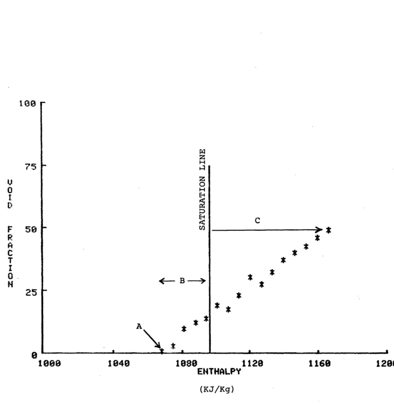
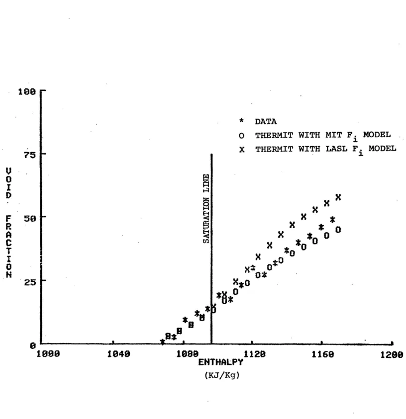
typical void fraction plot (Figure 3.1), three distinguishing features can be identified. The first is the point where boiling begins, point A. This point can be used to validate

the boiling inception point of the vapor generation model. The second feature is region B in which the slip ratio is nearly equal to 1.0 so that the void fraction is independent of Fi. Consequently, the subcooled vapor generation rate

can be verified in this region. The third feature is region C in which the vapor generation rate is independent of the flow conditions, so that the void fraction will be determined by the interfacial momentum exchange model. Therefore in this region, Fi can be assessed using the data. Thus, with a

z H O 0 H U) - B > A * 1 1880 * C * * * * % ** a ENTHALPY 1120 (KJ/Kg)

Figure 3.1 Typical Void Fraction versus Enthalpy Data 108 75 V 1 0_I D: F R A C T I 0 H 58 25 0 1800 S 1849 a 1160 a 1289 -, ml - -- m ~ - -- - .i

proper interpretation of the physical situation, the vapor generation rate and the interfacial momentum exchange rate can be evaluated using steady-state, one-dimensional void fraction data.

In the actual testing of THERMIT a large number of

experimental cases have been used. In all cases, the subcooled boiling model described in Appendix A and the M.I.T.

inter-facial momentum exchange model described in Appendix B have been used. For many cases, the LASL interfacial momentum exchange model has also been employed in order to investigate the sensitivity of the results to this model. All of the comparison cases are presented in Appendix D and only a few examples are discussed here. Table 3.2 summarizes all the experiments used in this investigation.

The first experimental comparisons have been performed using the data of Maurer (12). These data have been taken for high pressure water (1200-2000 psia) with a variety of mass

fluxes (0.4-4.0 Mlb/hr ft2), and heat fluxes (0.1-1.2 MBtu/hr ft2₎

in a 27 inch long rectangular test section (Dh = 0.18 inches). These data have been compared to THERMIT predictions and,

overall, the agreement between the two is very good. As seen in Figure 3.2, the code predictions for this case are in good agreement over the entire boiling length. The start of

boiling is predicted correctly as is the void fraction at high qualities. These trends are also observed for the other Maurer

TABLE 3.2

TEST CONDITIONS FOR ONE-DIMENSION STEADY-STATE DATA

Pressure Hydraulic Mass Flux Heat Flux Inlet

Test Range Diameter Range Range Subcooling (psia) (in) [Mlb/hr ft2) (MBtu/hr ft (Bt /lb)

(Btu/lb) Maurer 1200-1600 0.16 0.4- 0.9 0.09- 0.6 63 - 150 Christen- 400-1000 0.7 0.47-0.7 0.06- 0.16 4 - 30 sen Marcha- 260-615 0.444 0.44- 1.1 0.015-0.08 4 - 27 terre Bennett 1000 0.497 0.49-3.82 0.18-0.56 31 - 63

* Data

o THERMIT with

mIT

f4, 4' rl · _ 4 '1 , %.. ' -T JT 0 0 *0 0 0 1360 ENTHALPY (KJ/Kg)

Figure 3.2 Void Fraction Versus Enthalpy - MIaurer Case 214-3-6

75 U 0 I () Mode 1 F R A C T I 0 N 50 25 z H z o H E U.) * 0 1000 r $ 1180 1549 1728 1900 l- -- -- -- - & 1

6

cases which have been studied. Hence, the comparisons with this data would indicate that both the vapor generation model and the M.I.T. interfacial momentum exchange model are indeed correct.

However, the good agreement found in the above comparisons is not necessarily seen in all the cases which have been analyzed. For example, the comparisons between THERMIT and the data of

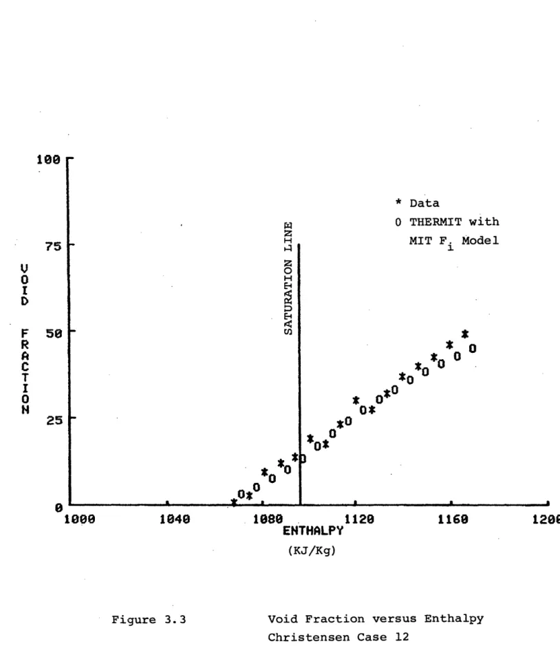
Christensen (13) show some minor discrepencies. This data has been taken in a 50 inch rectangular test section

(Dh = 0.7 inch) for a range pressures (400 - 1000 psia), mass fluxes (0.4 - 0.7 Mlb/hr ft2) and heat fluxes (0.07 - 0.16 MBtu/ hr ft2). A typical comparison curve is seen in Figure 3.3. In

this case, the code predictions are in fairly good agreement with the data, although there are some differences. A second comparison case is shown in Figure 3.4. The only difference in test conditions between this case and the previous one is the amount of inlet subcooling. Yet, in this case the measure-ments are not well predicted by THERMIT over the entire boiling length. The start of boiling and the amount subcooled vapor production coincide with the data, but the void fraction at high qualities is underpredicted by THERMIT. However, a com-posite curve of both cases (Figure 3.5) shows that at high qualities the void fraction measurements show considerable scatter. This result indicates some type of dependency on the inlet subcooling. On the other hand, the THERMIT

z H H E-4 E U) *o0 O . * Data O THERMIT with MIT F. Model I * 0 * 0*0 0* *0 '0 3 1080 1129 ENTHALPY (KJ/Kg) 1160

Figure 3.3 Void Fraction versus Enthalpy Christensen Case 12 100 75 V 0 I I D F R A C T I 0 50 25 0 1000 1040 1208 I -r -- · m ~~~~-iii·i· - _ -II-- I I

I-* Data O THERMIT with MIT F. Model 1 * ** * 0 *0t 0 0 0 1120

Figure 3.4 Void Fraction versus Enthalpy Christensen Case 13 75 U 0 1 D F R A C T I 0 N 50 25 * *I * * * H H H 0* o0 0 0 *_ 0o 0 1000 1040 1080 ENTHALPY (KJ/Kg) 1160 12800 _ I __ __ __ -I I - 1

* Data O THERMIT with MIT F. Model 1 :*0 ° * * * * 0 * It to 0 *: t* *0 0 * O

0*

Figure 3.5 Void Fraction versus Enthalpy Composite of Chrsitensen Cases 12 and 13 t0 75 V 0 I D 50 F R A C T I 0 H z H Z O H H C:1 E U) 0 1008 (KJ/Kg)

predictions show no dependence on the inlet subcooling which is what one might expect. Hence, it is difficult to assess the correct high quality behavior based on this data alone. A third set of measurements, those of Marchaterre (14), have also been compared with THERMIT. These measurements are for a 60 inch rectangular test section (Dh = 0.44 in.) with a range of pressures (160 - 600 psia), mass fluxes

(0.6 - 1.1 Mlb/hr ft2) and heat fluxes (0.04 - .25 MBtu/hr ft2). The comparison of these data show results similar to those seen above. For example, as seen in Figure 3.6 the code predictions for this case are in good agreement with the data. However, for another case, seen in Figure 3.7, the predictions fall below the data. The agreement in this case is not as good at high qualities, but is still good at low qualities. Hence, the boiling inception point and the amount of subcooled boiling are predicted correctly, but the void fraction at high qualities

tends to be underpredicted.

As discussed above, the void fraction at high qualities is a function of the interfacial momentum exchange rate. The above comparisons indicate that at high qualities the void

fraction is too low or, in other words, the slip ratio, is too high. In order to lower the slip ratio, the interfacial momentum exchange rate needs to be increased. A simple

compar-ison of the LASL model and the MIT model indicates that the LASL model predicts a transfer rate which is about a factor

* Data 0 THERMIT with MIT F. Model 1 0* 0 *0 *0 0 1080 1128 ENTHALPY (KJ/Kg)

Figure 3.6 Void Fraction versus Enthalpy Marchaterre Case 168 108 VI 0 I D F R A C T I 0 N 25 W z H ,4 z O H p Ul) * 0 0 0 0 0 1000 1040 1160 1280

* Data O THERMIT with MIT F. Model 1 * * * * 0 920 ENTHALPY (KJ/Kg) 0 0 969

Figure 3.7 Void Fraction versus Enthalpy Marchaterre Case 184 75 V 0 I D F R A C T I 0 N 25 0 0O Z H O H E-En 0 * 0 0 *0 0 0* 800 840 880 1ee9 _ m. . .

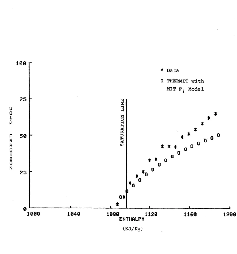
of 10 higher. Consequently, the Christensen and Marchaterre cases have also been analyzed using the LASL model in order to investigate the sensitivity of the void fraction predictions to this model (see Appendix D).

In general, the void fraction predictions with the LASL model are higher than the data at high qualities. This result,

illustrated in Figure 3.8, shows that the data lies between the predictions using the LASL model and those using the M.I.T. model. At low qualities the void fraction predictions are

nearly independent of the Fi model. Consequently, as expected, the interfacial momentum exchange rate only affects the void fraction at high qualities.

In order to assess the interfacial momentum exchange

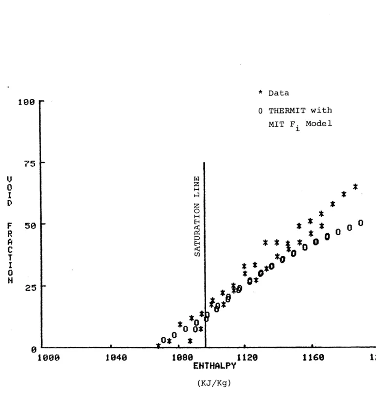
model, it is necessary to consolidate all of the data and then make a comparison with the code predictions. This process can be accomplished by plotting the superficial vapor velocity, Jv, versus the void fraction. A plot of this type is useful for comparing the data of a particular test section in which

the pressure, flow rate and power have been varied. For example, all of Christensen's data are plotted in Figure 3.9. The data show a definite trend with a certain amount of scatter. The code predictions are included in Figure 3.10 and it is seen that the two interfacial momentum exchange models bracket the data. The M.I.T. model slightly underpredicts the void fraction while the LASL model overpredicts the void fraction.

H

1008

Figure 3.8 Void Fraction Versus Enthalpy - Christensen Case 12

lea

N

1290

+ *e #$* I *0 + * *r 0 0 + 0 A x * + e v #X $e +0 $ @ a 0.4 Void Fraction

Figure 3.9 Vapor Superficial Velocity versus Void Fraction for Christensen Data.

# 2.0 1.5 s) * * Jv (m/' 1.0 0.5 0

x

LASL F. Model_I 2.5 2.0 1. 5 Jv (m/s) 1.0 0.5 tO

/

I

Figure 3.10 Vapor Superficial Velocity versus Void Fraction

Comparison of Data with THERMIT Predictions for Christensen Data.

Over the range of pressures (400 - 1000 psia) of these mea-surements, the M.I.T. model shows little sensitivity while the LASL model appears to be very sensitive to the pressure. Neither model could predict the scatter in the data, but each could be changed to lie closer to the majority of the data

(i.e., the M.I.T. model could be increased or the LASL model decreased).

In summary, the following conclusions can be drawn from the one-dimensional void fraction comparisons. First of all, the vapor generation model is found to accurately predict the point of boiling incipience and the amount of subcooled vapor for the majority of the data. Consequently, this model requires little, if any, improvement. The second conclusion

is that improvement is needed in the interfacial momentum exchange model. Either the M.I.T. model should be increased in value or the LASL model decreased in value. On the whole, the void fraction can be accurately predicted with THERMIT over the entire boiling length.

3.2.2 Clad Temperature Comparisons

The verification and assessment of the clad temperature predictive capabilities of THERMIT is the second step in the overall model evaluation strategy. The goal of this effort is to verify that the correlations in the heat transfer model accurately predict the clad temperature distribution when

from the fact that the heat transfer correlations depend on the specific flow conditions. Hence, if THERMIT is predicting

the correct flow conditions for a particular experiment, then the predicted clad temperatures should agree with the measured values provided the heat transfer correlations are valid.

Therefore, this heat transfer model evaluation effort relies on the work discussed in the previous section insofar as it

can be assumed that the flow conditions are accurately predicted. The THERMIT heat transfer model is a modified form of BEEST

heat transfer model (10) which constructs a complete boiling curve. As summarized in Table 3.3, a total of 10 heat transfer regimes are identified which include both pre-CHF and post-CHF conditions. Therefore, measurements over this wide range of conditions are needed to evaluate the heat transfer model.

The predictions of THERMIT have been compared with the data of Bennett (15). These measurements cover both pre-CHF and

post-CHF conditions and are, therefore, very useful for the present purposes. The data sets which have been used include a wide range of mass fluxes (0.5 to 3.8 Mlb/hr ft2 ) and heat fluxes (0.1 to 0.5 MBtu/hr ft). In each case the system pressure is 1000 psia and the test section is a 220 inch tube

(Dh = 0.5 inch) which is uniformly heated.

A total of 8 cases have been compared in this study. For each case the clad temperature measurements are compared to the code predictions. The complete set of comparison curves can be found in Appendix D, and only a few examples are

TABLE 3.3

SUMMARY OF HEAT TRANSFER REGIMES

regime:

Forced convection to single-phase liquid Natural convection to single-phase liqued Subcooled boiling Nucleate boiling Transition

High P, high G film boiling

Low P, high G film boiling

Low G film boiling

correlation: Sieder McAdams Chen Chen Interpolation between qCHF and qMSFB Groeneveld 5.7 Modified Dittus-Boelter Modified Bromley plus either McAdams vapor

or high flow film boiling Forced convection to

single-phase vapor Natural convection to single-phase vapor Sieder-Tate McAdams ihtr: 1 2 3 4 5 6 7 8 9 10

For each case, there are two regions of major interest from the viewpoint of the heat transfer model. These regions are identified in Figure 3.11 for a typical data set. In the

first region, I, the type of heat transfer is predominately nucleate boiling and, hence, measurements in this region can be used to validate the nucleate boiling heat transfer correlation. In the second region, II, either film boiling or single phase vapor are present and, consequently, the post-CHF heat transfer models can be evaluated in this region. The CHF correlation can also be verified by noting the location of the temperature excursion. Hence, the heat transfer model

can be validated in three parts, i.e., pre-CHF, post-CHF and CHF location.

For example, the data of case 5394 are compared with THERMIT predictions in Figure 3.12. In the pre-CHF regime, the code

consistently predicts a slightly larger value for the wall temperature than the data shows. This result indicates that the heat transfer coefficient is too low, but the error is well within the accuracy of the correlation. It is also seen that CHF is predicted to occur closer to the inlet than is actually observed. The difference in location of the CHF points is approximately 10% of the boiling length which again is within the limits of the CHF correlation. In the post-CHF region, the code predictions are in excellent agreement with the data. On the whole, the code can reasonably predict the wall temperatures for this case.

I

:HF Location

20 40 60 80 100 120 140 160 180 200 220 Axial Height (inches)

Figure 3.11 Typical Wall Temperature versus Axial Height Curve

1050 950 X 0 (V w ro ~--CD w a) E-H H Cd l3l-850 750 650 550 He f- II - ip

THERMIT\ Data a i a . . I - , , .- _. . I 20 40 60 80 100 120 140 160 180 200 220 Axial Height

Figure 3.12 Wall Temperature versus Axial Height Bennett Case 5394 1050 950 o₀ Cd 0 ; H_cov r:4 a) P I-I r-i (d 59-850 750 650 550 0 (inches)

A second comparison case is illustrated in Figure 3.13. Once again, THERMIT predicts both slightly higher wall temper-atures in the nucleate boiling regime and an earlier occurrence of CHF. However, in the post-CHF regime the code does not

accurately predict the wall temperatures. In this case, the heat transfer coefficient is too large except for a region near the exit. This result indicates that a problem may exist in the model and in particular the choice of the heat transfer correlation in this regime needs further evaluation.

The results of the 8 comparisons can be summarized as follows. In the nucleate boiling regime, the heat transfer model underpredicts the heat transfer coefficient and conse-quently, the wall temperature predictions are slightly larger

than the data. Better agreement is found in this regime for cases with a lower mass flux. The CHF location is consistently predicted to occur earlier than the observed value and the

error in this prediction is approximately 10%. An error of this magnitude is not excessive, but improvement can be sought. In the post-CHF regime, good to poor agreement is found between the predictions and the data. At low mass fluxes, the

agreement is poor and this problem indicates an area which requires further study.

THERMIT Data 0 20 40 60 Figure 3.13 * t. . t I X a |.I I I 80 100 120 140 160 180 200 220 Axial Height (inches)

Wall Temperature versus Axial Height Bennett Case 5273 1050 950 850 750 0o a) r4 a) P H r-r-q IlO 650 550 -_

I