Detecting hazardous intensive care patient episodes using real-time mortality models

(1)

Detecting Hazardous Intensive Care Patient

Episodes Using Real-time Mortality Models

by

MAS

Caleb Wayne Hug

S.M., Massachusetts Institute of Technology (2006)

B.S., Whitworth College (2004)

Submitted to the Department of Electrical Engineering and Computer

Science

in partial fulfillment of the requirements for the degree of

Doctor of Philosophy in Computer Science

at the

MASSACHUSETTS INSTITUTE OF TECHNOLOGY

June 2009

@

Massachusetts Institute of Technology 2009. All rights reserved.

A uthor ...

Department of Electrical Engineering and Computer Science

May 19, 2009

Certified by....

Peter Szolovits

Professor

Thesis Supervisor

/17?

Accepted by ....

Terry P. Orlando

Chairman, Department Committee on Graduate Students

SACHUSETTS INSTiTTE OF TECHNOLOGY

AUG 0

7 2009

LIBRARIES

6'

-7l

(2)

(3)

Detecting Hazardous Intensive Care Patient Episodes Using

Real-time Mortality Models

by

Caleb Wayne Hug

Submitted to the Department of Electrical Engineering and Computer Science on May 18, 2009, in partial fulfillment of the

requirements for the degree of Doctor of Philosophy in Computer Science

Abstract

The modern intensive care unit (ICU) has become a complex, expensive, data-intensive environment. Caregivers maintain an overall assessment of their patients based on important observations and trends. If an advanced monitoring system could also reliably provide a systemic interpretation of a patient's observations it could help caregivers interpret these data more rapidly and perhaps more accurately.

In this thesis I use retrospective analysis of mixed medical/surgical intensive care patients to develop predictive models. Logistic regression is applied to 7048 develop-ment patients with several hundred candidate variables. These candidate variables range from simple vitals to long term trends and baseline deviations. Final models are selected by backward elimination on top cross-validated variables and validated on 3018 additional patients.

The real-time acuity score (RAS) that I develop demonstrates strong discrimi-nation ability for patient mortality, with an ROC area (AUC) of 0.880. The final model includes a number of variables known to be associated with mortality, but also computationally intensive variables absent in other severity scores. In addition to RAS, I also develop secondary outcome models that perform well at predicting pressor weaning (AUC=0.825), intraaortic balloon pump removal (AUC=0.816), the onset of septic shock (AUC=0.843), and acute kidney injury (AUC=0.742).

Real-time mortality prediction is a feasible way to provide continuous risk assess-ment for ICU patients. RAS offers similar discrimination ability when compared to models computed once per day, based on aggregate data over that day. Moreover, RAS mortality predictions are better at discrimination than a customized SAPS II score (Day 3 AUC=0.878 vs AUC=0.849, p < 0.05). The secondary outcome mod-els also provide interesting insights into patient responses to care and patient risk profiles. While models trained for specifically recognizing secondary outcomes consis-tently outperform the RAS model at their specific tasks, RAS provides useful baseline risk estimates throughout these events and in some cases offers a notable level of pre-dictive utility.

Thesis Supervisor: Peter Szolovits Title: Professor

(4)

(5)

Acknowledgments

The research described in this thesis was funded in part by the National Library of Medicine (training grant LM 07092) and the National Institute of Biomedical Imaging and Bioengineering (grant R01 EB001659).

Many people helped make this work possible. I would first like to thank my lovely wife Kendra. She sacrificed many evenings to the time sink that graduate school can easily become. Her friendship, support, perspective (and food!) made the past five years an enjoyable journey - helping through the difficult moments and adding

immeasurably to the joyous times. Kendra and I welcomed our first child, Hannah, during my time at MIT. The opportunity to witness the miracle of life and a child's first exploration of the world is an experience that I relish and something that has renewed my appreciation for many of the simplest things in life and inspired my work. My research advisor, Peter Szolovits, was instrumental in guiding the research presented in this thesis. He allowed me the freedom and responsibility to pursue my own research directions. Many of the resulting digressions and tangents were invaluable contributions to my educational experience. But whenever I had questions, I could count on prescient insight and the rich experiential advice that stems from his illustrious career in medical informatics.

I would also like to acknowledge my other committee members, including Bill Long, Roger Mark, and Lucila Ohno-Machado. Each member provided constructive conversations, helpful advice, and excellent feedback regarding the research presented in this thesis. I am especially grateful for Bill's patience in listening to me as I bounced ideas off of him or sometimes ranted about data problems.

A number of other individuals at MIT also helped me with this work. Tom Lasko's friendship and advice was an immense encouragement to me as I first began to explore the field of medical informatics. Andrew Reisner provided helpful information for many of my clinical questions and was always a joy to talk with. Gari Clifford and Mauricio Villarroel provided much assistance with the data used in this study and provided many enjoyable conversations. I am blessed to consider all of these individuals my friends.

Furthermore, I would be remiss not to mention several others who played an essential role in my successful completion of this work. Kent Jones, Susan Mabry, and Howard Gage - computer science and mathematics faculty from Whitworth College - went out of their way to challenge and encourage me. While the past five years seemed to have passed so quickly, my parents and brothers (especially my oldest brother Joshua) were also wonderful sources of encouragement to me during the times with no apparent end in sight.

During my time at MIT I spent three years living as a graduate resident tutor in an undergraduate dorm. Living with the students of Conner 4 was a great experience and complimented my MIT education in many ways. While I'm excited to finally move off campus, I will miss the energy and community that characterize this group of talented young adults.

Studying in historic New England has nurtured a strong respect for my country. My story is a testament to the exceptionalism of the United States, a country built

(6)

on reverence for human liberty and filled with endless opportunities. As my graduate student tenure comes to an end, I marvel at the great privilege of graduate education in this country - an easily overlooked privilege made possible by the generous tax dollars of U.S. citizens. I will not forget the investment that my country has made.

Finally, I would like to thank my Heavenly Father. He has given me a rich life

- blessed me with a wonderful family, a healthy body, and all of my worldly needs. Furthermore, He has challenged me with opportunities to grow personally, spiritually, and academically at a renowned institution. I could not ask for more opportunity. As king Solomon wrote in the book of Proverbs, "It is the glory of God to conceal a thing; but the honor of kings is to search out a matter." For a farm boy from the sticks, I indeed feel like I have been in the company of kings. And I believe uncovering the wonder of mathematics and the intricacies of the human body offer but a glimpse of the glory of God.

(7)

List of Figures

3-1 Observation frequency histograms . ... . 31

3-2 Histograms for demographic information . ... 45

3-3 SAPS II Variables ... .. ... 46

3-4 SAPS II Variables (cont) ... ... 47

3-5 ICU Readmissions ... 48

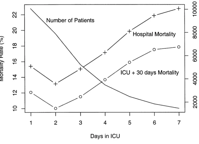
3-6 Patient mortality rate versus ICU day . ... 49

3-7 Patient mortality rate versus ICU day: Final dataset . ... 52

5-1 SDAS model selection using cross-validation . ... 68

5-2 SDAS model selection ... ... 69

5-3 SDAS ROC curve (development data) . ... 73

5-4 DASn model selection (all development data) . ... 76

5-5 Ranked comparison of DASn inputs . ... 82

5-6 DASn ROC curves (development data) . ... 84

5-7 SDAS ROC curves (validation data) . ... 88

5-8 DASn ROC curves (validation data) ... 89

5-9 Calibration plots for SDAS day 1 and DAS1 (validation data) ... 92

5-14 RAS model selection using cross-validation . ... 98

5-15 RAS model selection (all development data) . ... 101

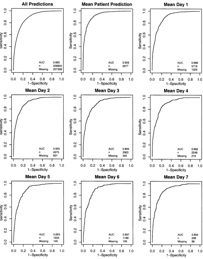
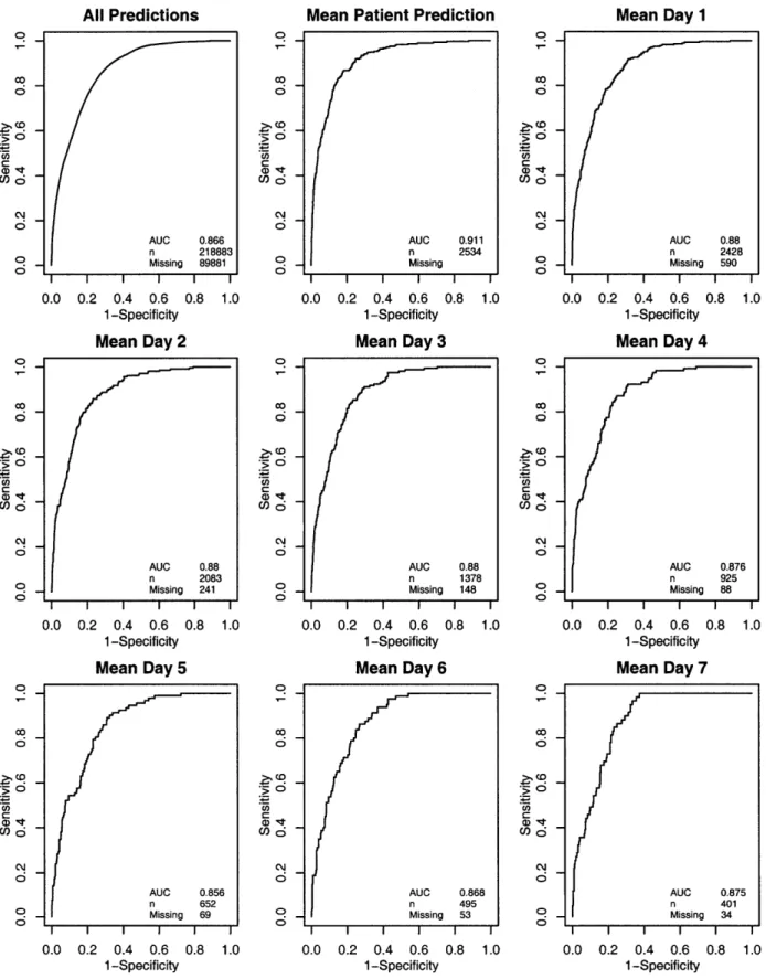
5-16 RAS ROC curves (development data) . ... 102

5-17 RAS ROC curves (validation data) ... . 103

5-18 RAS calibration plots (validation data) . ... . . . . 105

5-19 RAS calibration plots, days 2 and 3 (validation data) . ... 106

5-20 RAS calibration plots, days 4 and 5 (validation data) . ... 107

5-21 SAPSII, ROC curves ... ... 110

5-22 SAPSII, calibration plots, days 1 through 3 ... 113

5-23 SAPSIIa calibration plots, days 4 and 5 . ... 114

5-24 AUC versus day, first 5 ICU days (development data) . ... 116

5-25 AUC versus day, first 5 ICU days (validation data) . ... 116 5-26 AUC versus day, patients with ICU stays > 5 days (development data) 117 5-27 AUC versus day, patients with ICU stays > 5 days (validation data) . 117

(12)

6-1 6-2 6-3 6-4 6-5 6-6 6-7 6-8 6-9 6-10 6-11 6-12 6-13 6-14 6-15 6-16 6-17 6-18 6-19 6-20 6-21 6-22 6-23 6-24 6-25 6-26 6-27 6-28 6-29 6-30 6-31 6-32 6-33 6-34 6-35 6-36 6-37 6-38 6-39 6-40 6-41 6-42 6-43 6-44 6-45

Pressor-infusion episode lengths . . . .. PWM example annotations . . . .... PWM model selection (all development data) . . PWM ROC curve (development data) . . . . PWM predictive values (development data) . . . PWM prediction context surrounding successful p PWM prediction context surrounding successful p PWM example annotations with predictions . .

PWM calibration plot . ...

PWM ROC curve (validation data) . . . . PWM predictive values (validation data) . . ..

PWM prediction context surrounding successful p PWM prediction context surrounding successful p Pressor-infusion episode lengths . . .... ... PWLM example annotations ...

PWLM model selection (all development data) . . . .

PWLM ROC curve (development data) . . . .. PWLM predictive values (development data) . . . . . PWLM prediction context surrounding HDFR . . . .

PWLM example annotations with predictions . . . . . PWLM calibration plot . ...

PWLM ROC curve (validation data) . . . ... PWLM predictive values (validation data) . . . . PWLM prediction context surrounding HDFR . . . . IABP episode lengths . ...

BPWM example annotations ...

BPWM model selection (all development data) . . . .

BPWM ROC curve (development data) . . . .. BPWM predictive values (development data) . . . . . BPWM prediction context surrounding IABP removal BPWM prediction context surrounding IABP removal BPWM example annotations with predictions . . . . . BPWM calibration plot . ...

BPWM ROC curve (validation data) . . . ... BPWM predictive values (validation data) . . . . BPWM prediction context surrounding IABP removal BPWM prediction context surrounding IABP removal Septic shock onset warning lengths . . . ... SSOM example annotations ...

SSOM model selection (all development data) . . . .

SSOM ROC curve (development data) . . . .. SSOM predictive values (development data) . . . . . SSOM prediction context surrounding HDFR . . . .

SSOM prediction context surrounding HDFR . . . . SSOM example annotations with predictions . . . . . resso resso resso resso resso .. . . . . 129 .. . . . . 130 . . . . . . . 131 .. . . . . 135 .. . . . 136 r weans .... . 137 r weans .... . 138 . . . . . . . 138 . . . . . . 141 . . . . . . 142 . . . . . . 142 r weans .... . 143 r weans .... . 143 . . . . . . 148 . . . . . . 149 . . . . . . . . 150 . . . . . . 152 . . . . . . . 153 . . . . . . . . 154 . . . . . . . 154 . . . . . . 156 . . . . . . 157 . . . . . . . 157 . . . . . . . . 158 . . . . . . 164 . . . . . . 164 . . . . . . . . 165 . . . . . . 168 . . . . . . 169 . . . . 170 . . . . . 171 . . . . . . 171 .. . . . 172 .. . . . . 173 . . . . . . 173 . . . . 174 . . . . 174 .. . . . . 179 .. . . . . 180 . . . . . . . . 181 .. . . . . 184 . . . . . . 184 . . . . . . . 185 . . . . . . . 186 . . . . . . . 186

(13)

6-46 6-47 6-48 6-49 6-50 6-51 6-52 6-53 6-54 6-55 6-56 6-57 6-58 6-59 6-60 6-61 6-62 6-63 6-64 6-65 6-66 6-67 6-68 6-69 C-1 C-2 C-3 C-4 C-5 C-6 C-7 C-8

Ventilator type recording frequency . . . .

Joint density: change in pressors and time Joint density: change in pressors and time Joint density: change in pressors and time Joint density: change in pressors and time DAS1 model selection stage 1

DAS2 model selection stage 1 DAS3 model selection stage 1 DAS1 model selection stage 2 DAS2 model selection stage 2 DAS3 model selection stage 2 DAS4 model selection stage 2 DAS5 model selection stage 2

(day (day (day (day (day (day (day (day (high doses) . . . (medium-high dose (died) . . . . (lived) ... SSOM calibration plot . ... ...

SSOM ROC curve (validation data) . . . . SSOM predictive values (validation data) . . . . SSOM prediction context surrounding HDFR . . . . SSOM prediction context surrounding HDFR . . . . Creatinine Measurement Intervals . . . . Acute kidney injury onset warning lengths . . . . . AKIM example annotations . . . . AKIM model selection (all development data) . . . . AKIM ROC curve (development data) . . . . AKIM predictive values (development data) . . . . . AKIM prediction context surrounding kidney injury . AKIM prediction context surrounding kidney injury . AKIM example annotations with predictions . . . . . AKIM calibration plot (validation data) . . . . AKIM ROC curve (validation data) . . . . AKIM predictive values (validation data) . . . . AKIM prediction context surrounding kidney injury . AKIM prediction context surrounding kidney injury .

. . . . . 250 . . . . . 251 . . . . . 252 . . . . . 253 . . . . . . . . . . . 254 . . . . . . . . . . 255 . . . . . 256 . . . . . . . . . . . . 257

E-1 Model outputs for patient 13319 E-2 Model outputs for patient 23047 E-3 Model outputs for patient 14386 E-4 Model outputs for patient 23335 E-5 Model outputs for patient 5872 E-6 Model outputs for patient 21521 E-7 Model outputs for patient 7272 E-8 Model outputs for patient 23600 E-9 Model outputs for patient 931 E-10 Model outputs for patient 8451 E-11 Model outputs for patient 14302 264 265 266 267 268 269 270 271 272 273 274 . . . . . 188 . . . . . 189 . . . . . 189 . . . . . 190 . . . . . 191 . . . . . 197 . . . . . 198 . . . . . 199 . . . . . 201 . . . . . 203 . . . . . 203 . . . . . 204 . . . . . 204 . . . . . 205 . . . . . 207 . . . . . 208 . . . . . 208 . . . . . 209 . . . . . 209 . . . . . 213 . . . . . 216 s) . . . 217 . . . . . 218 . . . . . 218

(14)

E-12 Model outputs for patient 1224 . . . . . E-13 Model outputs for patient 8929 . . . . . E-14 Model outputs for patient 20113 . . . . . E-15 Model outputs for patient 10855 . . . . . E-16 Model outputs for patient 18687 . . . . . E-17 Model outputs for patient 13538 . . . . . E-18 Model outputs for patient 14692 . . . . . E-19 Model outputs for patient 4754 . . . . . E-20 Model outputs for patient 24019 . . . . . E-21 Model outputs for patient 12483 . . . . . E-22 Model outputs for patient 22716 . . . . . E-23 Model outputs for patient 13642 . . . . . E-24 Model outputs for patient 23224 . . . . . E-25 Model outputs for patient 5947 . . . . . E-26 Model outputs for patient 21799 . . . . . E-27 Model outputs for patient 6946 . . . . . E-28 Model outputs for patient 23877 . . . . . E-29 Model outputs for patient 864 . . . . E-30 Model outputs for patient 7803 . . . . . E-31 Model outputs for patient 13765 . . . . . E-32 Model outputs for patient 1168 . . . . . E-33 Model outputs for patient 8817 . . . . . E-34 Model outputs for patient 20353 . . . . . E-35 Model outputs for patient 10776 . . . . . E-36 Model outputs for patient 19108 ... E-37 Model outputs for patient 13032 . . . . . E-38 Model outputs for patient 14466 . . . . . E-39 Model outputs for patient 4690 . . . . . E-40 Model outputs for patient 24847 . . . . . F-1 PWM model selection using cross validation F-2 PWM final feature set performance on cross F-3 PWLM model selection using cross validatio

. ... . 275 . ... . 276 . ... . 277 ... ... . 278 . ... . 279 ... ... . 280 . ... . 281 . ... . 282 ... ... . 283 . ... . 284 ... ... . 285 ... ... . 286 ... ... . 287 ... ... . 288 .... ... . 289 . ... . 290 .... ... . 291 .. ... . 292 . ... . 293 ... ... . 294 ... ... . 296 . ... . 297 ... ... . 298 ... ... . 299 ... ... . 300 ... ... . 301 . ... . 302 . ... . 303 ... ... . 304 . . . . . . . . . . 306 validation folds ... 307 n . . . . .

F-4 PWLM final feature set performance on cross validation folds F-5 BPWM model selection using cross validation . . . . F-6 BPWM final feature set performance on cross validation folds F-7 SSOM model selection using cross validation . . . . F-8 SSOM final feature set performance on cross validation folds F-9 AKIM model selection using cross validation . . . . F-10 AKIM final feature set performance on cross validation folds

308 309 310 311 312 313 314 315

(15)

List of Tables

Continuous and Ordinal ChartEvent Variables . . . . Categorical ChartEvent variables . . . . MedEvent variables (Intravenous Medications) . . . .

IOEvents variables ... ...

ItemIDs used for summary IO variables . . . . TotalBalEvents variables . . . . . . . ..

Demographic Variables . . . . . . . . . ...

Derived Variables . ... . . ... Variables from Literature ...

Variables with Range and Baseline Deviation Calculations Hospital and ICU Admissions . . . .. Outcome Variables . . . . . . . . . ..

Final Dataset: Entire Patient Exclusions . . . . Final Dataset: Partial Patient Exclusions . . . . Preprocessed Data . . . . . . . . . . ..

4.1 SAPS II Variables ...

Final dataset description . . . . . . . . . ....

Real-time data ... ... ...

Aggregated Daily Data ... ... . .. ...

SDAS Hosmer-Lemeshow H risk deciles (all days) . . . . SDAS Hosmer-Lemeshow C probability deciles (all days) . . . . . SDAS bootstrapped goodness of fit statistics (development data) DASn model characteristics (development data) . . . . DAS1 bootstrapped goodness of fit statistics . . . . DAS2 bootstrapped goodness of fit statistics . . . . DAS3 bootstrapped goodness of fit statistics . . . . DAS4 bootstrapped goodness of fit statistics . . . .. DAS5 bootstrapped goodness of fit statistics . . . . Hosmer-Lemeshow calibration summaries for SDAS and DASn . . SDAS Hosmer-Lemeshow H deciles of risk (validation data) . . . DAS1 Hosmer-Lemeshow H deciles of risk (validation data) . . RAS Hosmer-Lemeshow calibration (development data) . . . . . RAS bootstrapped goodness of fit statistics (development data) . RAS Hosmer-Lemeshow calibration (validation data) . . . . 3.1 3.2 3.3 3.4 3.5 3.6 3.7 3.8 3.9 3.10 3.11 3.12 3.13 3.14 3.15 . . . . 32 . . . . 34 . . . . 36 ... . 37 . . . . 38 . . . . 39 . . . . 39 . . . . 41 ... . 42 . . . . 43 . . . . 48 . . . . 50 . . . . 50 . . . . 51 . . . . 51 5.1 5.2 5.3 5.4 5.5 5.6 5.7 5.8 5.9 5.10 5.11 5.12 5.13 5.14 5.15 5.16 5.17 5.18 . . . 66 .. . 66 .. . 67 . . . 73 . . . 74 . . . 74 . . . 83 . . . 85 . . . 85 . . . 86 . . . 86 . . . 86 . . . 87 . . . 90 . . . 90 . . . 100 . . . 100 . . . 101

(16)

5.19 RAS H statistic deciles of risk ... ... 104

5.20 SAPSII, calibration statistics . ... ... . . . 109

5.21 SAPSIIa bootstrapped goodness of fit statistics, day 1 (dev data) . . . 109

5.22 SAPSII, bootstrapped goodness of fit statistics, day 2 (dev data) . . 111

5.23 SAPSII, bootstrapped goodness of fit statistics, day 3 (dev data) . . . 111

5.24 SAPSII, bootstrapped goodness of fit statistics, day 4 (dev data) . . 111

5.25 SAPSIIa bootstrapped goodness of fit statistics, day 5 (dev data) . . . 112

5.26 SAPS II customization AUC performance . ... 115

5.27 Model coverage on validation data . ... . 115

5.28 Calibration statistics for daily model comparisons (development data) 118 5.29 Calibration statistics for daily model comparisons (validation data) 118 5.30 RAS DeLong AUC significance tests (days 1 through 5) ... 118

5.31 RAS DeLong AUC significance tests (5+ day patients) ... 119

6.1 PWM data ... .. . ... 130

6.2 PWM Hosmer-Lemeshow H risk deciles (development data) ... 134

6.3 PWM Hosmer-Lemeshow C probability deciles (development data) . . . 134

6.4 PWM Hosmer-Lemeshow H risk deciles (validation data) ... 139

6.5 PWM Hosmer-Lemeshow C probability deciles (validation data) . . . . 140

6.6 PWLM data ... . ... .. 147

6.7 PWLM Hosmer-Lemeshow H risk deciles (development data) ... 150

6.8 PWLM Hosmer-Lemeshow C probability deciles (development data) . . 152

6.9 PWLM Hosmer-Lemeshow H risk deciles (validation data) . ... 155

6.10 PWLM Hosmer-Lemeshow C probability deciles (validation data) . . . . 156

6.11 BPWM data ... . . . .. ... 163

6.12 BPWM Hosmer-Lemeshow H risk deciles (development data) ... 167

6.13 BPWM Hosmer-Lemeshow C probability deciles (development data) .. 168

6.14 BPWM Hosmer-Lemeshow H risk deciles (validation data) . ... 170

6.15 BPWM Hosmer-Lemeshow C probability deciles (validation data) . . . . 172

6.16 SIRS Variables ... 178

6.17 SSOM data ... . . . ... 179

6.18 SSOM Hosmer-Lemeshow H risk deciles (development data) ... 183

6.19 SSOM Hosmer-Lemeshow C probability deciles (development data) . 183 6.20 SSOM Hosmer-Lemeshow H risk deciles (validation data) ... 187

6.21 SSOM Hosmer-Lemeshow C probability deciles (validation data) . . . . 187

6.22 RIFLE Classification Scheme ... ... 196

6.23 Estimated baseline creatinine ... ... 196

6.24 AKIM data ... ... ... ... 197

6.25 AKIM Hosmer-Lemeshow H risk deciles (development data) ... 202

6.26 AKIM Hosmer-Lemeshow C probability deciles (development data) . . 202

6.27 AKIM Hosmer-Lemeshow H risk deciles (validation data) . ... 206

6.28 AKIM Hosmer-Lemeshow C probability deciles (validation data) . . . . 206

(17)

D.1 DASi: Hosmer-Lemeshow Goodness of Fit Test: Risk Deciles ... 259 D.2 DAS2: Hosmer-Lemeshow Goodness of Fit Test: Risk Deciles ... 260 D.3 DAS3: Hosmer-Lemeshow Goodness of Fit Test: Risk Deciles .... . 260 D.4 DAS4: Hosmer-Lemeshow Goodness of Fit Test: Risk Deciles .... . 260 D.5 DAS5: Hosmer-Lemeshow Goodness of Fit Test: Risk Deciles .... . 261

(18)

(19)

Chapter 1 Introduction

The modern intensive care unit (ICU) has become a complex, expensive, data-intensive environment. In this environment - where physician decisions often make the dif-ference between life and death - tools that help caregivers interpret patterns in the data and quickly make the correct decision are essential. My objective in this research is to develop models that, given a set of observations, provide a systemic "understanding" of a patient's medical well-being and assist physicians in making more informed decisions. I use a data-driven approach to model the complex patient system by considering variables that range from therapeutic interventions to simple vitals to complex trends. Specifically, I develop several mortality models and compare them against a real-time mortality model. I then compare and contrast the ability of mortality models to predict acute patient events with models that were specialized to predict specific events. If real-time risk models can be successfully developed, physi-cians could have an immediate alert of jeopardized patient state - providing valuable time to intervene - or an indicator of a particular treatment regime's benefit to an individual patient.

1.1 Overview

While doctors routinely do an outstanding job of matching complex patterns observed in patient data to an applicable set of diagnoses and treatments, they are not perfect. Patients admitted to ICUs - a particularly vulnerable category of patients - require close monitoring due to an increased probability of life threatening events. The close attention of caregivers, necessary to provide high quality care, clearly exposes patients to the human errors known to be common in health care [40]. In fact, Rothschild et al. found that ICU patients suffer a large number iatrogenic injuries, especially failure to carry out intended treatment correctly [71]. A system that understands the patient's progression could potentially catch dangerous episodes and ultimately increase caregiver vigilance.

(20)

CHAPTER 1. INTRODUCTION

errors. These shortages are particularly evident in the ICU. One survey conducted in 2000 found that the nurse vacancy rate in critical care, at 14.6%, was higher than other locations [30]. In order to fill vacancies, temporary staff are commonly used in many hospitals. Furthermore, projections indicate that the current shortage of intensivists will shortly be a crisis [41]. In the ICU, the potential for information technology and medical informatics to supply decision support, enhance efficiency, and generally improve quality by utilizing relevant data is well understood (e.g., see [36]). In fact, companies such as VISICU (recently acquired by Philips Medical Systems) have emerged that seek to leverage the intensivist shortage by allowing a single intensivist to monitor up to 100 patients through a remote environment. A system that can effectively interpret a patient's data could help reduce the burden placed on caregivers and, as a result, help alleviate the intensivist shortage.

Despite the theoretical promise of comprehensive patient monitors, reality might present a more dire picture. One recent review by Ospina-Tasc6n et al. [64] questions the utility of recent monitoring progress by pointing to the systemic lack of ran-domized controlled trials and argues that, of the few conducted, most show negative results. Besides the clear ethical problems with conducting randomized controlled trials on obviously helpful monitors (e.g.; electrocardiogram monitoring for patients with acute myocardial infarction), Ospina-Tascon6n's review raises many questions regarding the utility of investing in monitoring development. An alternative inter-pretation that might be inferred from such criticisms of contemporary monitoring systems is that the systems are inadequate for the actual caregiver needs. Are ad-vanced monitoring devices really helpful, or do they simply overwhelm the nurses and physicians with useless information that do not ultimately benefit patients?

Current monitors do indeed come at a cost. Concerned about sensitivity, monitors often sacrifice specificity. The trade-off between sensitivity and specificity can be seen by the documented prevalence of false alarms [58, 89, 90, 57]. An ancillary burden from devices with low specificity and high sensitivity is excessive background sound

- Ryherd et al. found that the noise level in one neurological intensive care unit was significantly higher than recommended by the World Health Organization guide-lines [74]. Caregivers surveyed as part of Ryherd's study overwhelmingly indicated that the noise adversely affected them and their patients. The prevalence of audible false alarms indicate that the wealth of observations taken in the ICU are poorly understood at the monitoring level. The problem of better interpreting observations in order to increase specificity has attracted considerable attention, and recent work, such as that by Zong et al., has demonstrated methods for dramatically reducing false alarm rates [95]. Modern monitors are able to corroborate related signals in order to limit spurious alarms. Current approaches, however, generally focus on better alarms on individual signals rather than to fuse information together to reflect the underly-ing patient condition and produce warnunderly-ings such as suspected hypovolemia or septic shock.

(21)

1.2. OUTLINE OF THESIS

the ability to quickly search the Internet and find highly relevant information - it is only a matter of time before relevant medical knowledge will be highly accessible from the bedside. The insurmountable electronic medical record obstacle has even shown signs of abating with several large industry players making substantial investments in the personal health record (PHR) arena and releasing promising solutions such as the Microsoft HealthVault, Google Health, or Dossia's Indivo system [60, 20, 10, 22].

Current U.S. government trends also indicate large investments in standards-based electronic health information systems. As standards emerge for electronic health records, detailed patient history will be available. If this additional patient informa-tion can be synthesized, better and more customized care could result. In general, the emerging innovations in the field of informatics point to an environment where a wealth of useful data will be available at the ICU bedside for use in systems that automatically assist caregivers.

One approach to understanding a patient is to focus on the patient's risk of death. A real-time risk model - or real-time acuity model - could track important changes in a patient's risk profile. More volatile patient states presumably have patterns that are associated with a greater risk of mortality. A real-time acuity score could also provide more frequent outcome prognoses than the current daily severity of illness scores. Clinically, the value of a real-time acuity score remains uncertain. How should a patient's care change if the score changes from a 50% chance of survival to a 60% chance of survival? Such changes are unlikely to be useful in determining the patient's care. However, if the model could detect (1) acute deterioration in the patient's state or (2) insidious changes in state over the course of a day, then it could potentially help interpret abundant ICU data more rapidly and perhaps more accurately.

In this thesis, I investigate a real-time general acuity model for intensive care patients. The acuity model that I explore is based on a patient's risk of near-term mortality. I first contrast my real-time acuity model with daily acuity models and existing severity of illness scores, and then I examine the performance of my general acuity model in the context of secondary outcomes. For comparison, a variety of models that predict secondary outcomes directly are developed and discussed. Unlike existing daily scores, which generally emphasize simplicity, my models utilize a variety of computationally intensive inputs as well as caregiver interventions. Furthermore, in contrast to a daily point score, a real-time acuity score can offer a detailed summary of a patient's risk profile over time.

1.2 Outline of Thesis

This thesis is organized into the following chapters:

* Chapter 2 provides an overview of existing severity of illness scores with a particular focus on the role that time plays in severity of illness scores.

(22)

CHAPTER 1. INTRODUCTION

* Chapter 3 describes the data and the preparation of the data that I use to create and validate the predictive models that I consider in this report.

* Chapter 4 discusses the general methodological framework that I follow to create and validate the predictive models.

* Chapter 5 develops and describes three types of mortality models: (1) daily mortality models, (2) a stationary daily mortality model, and (3) a real-time mortality model.

* Chapter 6 examines models trained and validated on specific secondary out-comes and compares their performance with the performance of the real-time mortality model developed in Chapter 5.

* Finally, Chapter 7 concludes my thesis with a summary of the contributions that it makes to the field of medical informatics and a discussion regarding future work.

(23)

Chapter 2 Background

2.1 Severity of Illness Scores

One area where researchers have utilized large amounts of ICU data is the develop-ment of severity of illness scores. Over the past 20 years, there has been a growing interest in severity of illness scores and several mature options have emerged, including the Acute Physiology and Chronic Health Evaluation (APACHE) [39], the Simplified Acute Physiology Score (SAPS) [45], the Mortality Prediction Model (MPM) [52], and several more recent generations of each of these scores [37, 38, 44, 51, 46]. The APACHE score was constructed using an expert clinical panel to select variables and denote levels of severity for each. The SAPS metric was designed similarly to APACHE, but its designers sought to match the APACHE performance using a simpler (and less time consuming to calculate) model. The APACHE and SAPS metrics both provide a point score at 24 hours after admission that indicates the illness severity for the patient. The MPM model took a different approach, using a more objective, forward stepwise selection methodology to select important variables. Unlike APACHE and SAPS, the MPM provides the patient's mortality probability directly and was constructed for multiple time points: at admission and 24 hours af-ter admission. More recent MPM models have been constructed for 48 hours and 72 hours after admission [50]. Prominent severity of illness scores have been validated on large multi-center databases - or, in the case of SAPS and MPM, large international databases. Recent work by Ohno-Machado et al. in [63] provides a thorough review of severity of illness scores.

The original intent of severity scores was to compare groups of patients and to stratify patient populations between hospitals. Despite warnings from many of the original researchers and several studies (e.g., [76]), many caregivers have come to expect the availability of a severity score to assist them in treating individual patients. The fact is that despite their inadequacy for individual care, severity of illness scores are not going away [27]. Many researchers have validated the use of severity of illness scores in settings that deviate from their original design. Alternative settings

(24)

CHAPTER 2. BACKGROUND

have included populations such as coronary care patients or subarachnoid hemorrhage patients or days subsequent to the initial 24 hours after admission [80, 26, 79, 72]. The performance under these alternate settings has been generally moderate.

The underlying models behind existing severity metrics remain quite simplistic. Many of their original constraints are arguably unnecessary given the nearly ubiqui-tous availability of computing power today. The traditional advantage of SAPS, i.e., its simplicity, makes little difference in an environment where data are automatically collected and processed by a computer. In fact, using digital data, it is now feasible to include complicated derived features, such as long term trends or deviation from a patient's baseline, as possible inputs. Features that capture trends, patient-specific abnormalities, or important patterns in various observations should provide addi-tional insight into the patient's underlying stability. On the other hand, caregivers appreciate simple models because of their comprehensibility and they are hesitant to use decision support systems that they do not understand. Another advantage of simplicity is the ability to calculate scores from widely available observations allowing scores to be easily implemented across different hospitals and diverse patient popula-tions. In order to surmount the obstacles presented by a more abstruse system that requires advanced infrastructure for implementation, a real-time acuity score needs to offer clear benefits to the caregiver's daily tasks by providing sensitive but specific assessment calibrated for individual patients.

2.1.1 Organ Dysfunction Scores

While the intent of the general severity indexes has been to provide mortality risk assessment, complementary work has been done to develop organ dysfunction scores to assess patient morbidity. One such score, the sepsis-related organ failure assessment (SOFA) score, seeks to "describe a sequence of complications in the critically ill" [92, 91]. The SOFA score is limited to 6 organs by looking at respiration, coagulation, liver, cardiovascular, central nervous system, and renal measurements. For each organ, the score provides an assessment of derangement between 0 (normal) and 4 (highly deranged). One noteworthy feature of the SOFA score is that it uses the mean arterial pressure (MAP) along with vasopressor administration for the cardiovascular assessment. In contrast to the mortality risk provided by most severity of illness scores, the SOFA score aims to evaluate morbidity. Since its introduction, several studies have successfully applied the SOFA score to non-sepsis patients (e.g., trauma patients [1]) and the meaning of the SOFA acronym quickly morphed into Sequential Organ Failure Assessment.

Other organ dysfunction scores include the multiple organ dysfunction score (MODS), the logistic organ dysfunction score (LODS) and the multiple organ failure score

[56, 43, 21]. Differentiating itself from the intervention-dependent SOFA score, the MODS score relies on what its authors refer to as the "pressure adjusted heart rate"

(25)

pres-2.1. SEVERITY OF ILLNESS SCORES

sure to mean arterial pressure [56]. The LODS score was designed for use only during the first ICU day and combines the level of dysfunction of all organs into a sin-gle score. The association of organ dysfunction with mortality has prompted many papers to explore the use of organ dysfunction scores at predicting mortality with results that are, in general, only slightly worse than the general severity of illness scores [62, 18, 6, 48, 7, 96, 67, 86]. While the organ dysfunction scores are func-tionally similar to my objective in this research, the critical distinction is that I will approach the problem from the opposite direction; that is, I will look at a mortality model's ability to understand patient state whereas organ dysfunction scores were designed to reflect organ derangement and are often validated by their correlation with final patient outcome.

2.1.2 Machine versus Human

How do severity scores compare to humans? Relative performance between "objec-tive" scores and humans is a difficult question that several studies have examined. When physicians have a low prediction of ICU survival (< 10%), Rocker et al. found that the low prediction, often acted on by limiting life support, by itself predicts mor-tality better than the severity of illness metrics or organ dysfunction scores, thereby making the doctor's belief a self-fulfilling prophecy [68]. The advantage that physi-cians have at predicting mortality is supported by a variety of studies that show physicians generally outperform severity scores [83, 78, 76]. Comparisons between physicians and scoring systems all share the problem alluded to above: a physician's prognosis for an individual patient clearly influences the physician's actions. The coupling between a physician's prognosis and his or her actions is an unavoidable challenge inherent in the retrospective analysis of any intensive care episode. If the doctor is considered the gold standard, it is impossible to demonstrate improvement over his or her actions. Perhaps this observation, combined with prior experience, better calibration for individual patients, and consideration of factors not included in scoring systems is why physicians generally perform marginally better at predict-ing mortality. Some researchers, however, have argued from a resource utilization viewpoint that given what they consider to be reasonable performance from severity scores, automatic scores should be adopted as objective measures to prevent futile care in the costly ICU environment. It seems prudent that severity scores improve drastically - especially in terms of individual patient calibration - before such ac-tion is considered.

2.1.3 Modeling Survival

Most ICU outcome prediction models rely on logistic regression. For example, a variety of equations are available for SAPS and APACHE severity scores to convert the point score into a mortality probability. Logistic regression has the advantage of

(26)

CHAPTER 2. BACKGROUND

being straightforward and relatively easily to comprehend. Bayesian networks have also been used to better understand the structure of complex data. Such analysis has revealed interesting details about many complex systems. I have previously explored the application of survival models to an earlier release of the MIMIC II data. The

advantage that survival techniques have, however, is limited by the absence of quality follow-up data (in general I only know which patients die in the hospital). Given the limited follow-up information, my analysis indicated that survival models perform nearly the same as logistic regression models at predicting outcome, but the fitting routines for survival models are less stable.

2.1.4 The Role of Time

A number of researchers have explored using daily severity of illness metrics. In

1993, Le Gall et al. suggested that despite likely being too time-consuming for most ICUs, daily scores would be the most "efficient way to evaluate the progression of risk of death" [44]. Ru6 et al. found that the mortality prediction on the current-day was the most informative - in fact, the mortality probability at admission and on previous days did not improve performance from the current day's score [72]. The importance of the current-day mortality prediction that Ru6 et al. observed corrob-orates Lemeshow et al.'s finding that the most important features change between the admission MPM model and the 24, 48 and 72 hour MPM models. The logistic regression equation also changes between 24-hour intervals to reflect an increasing probability of mortality [50]. From their observations, Lemeshow et al. make the gen-eral observation that a patient in the ICU with a "steady" clinical profile is actually getting worse.

Several others have examined the sequential assessment of daily severity scores. In 1989, Chang notably found that, using a set of criteria along with daily APACHE II scores, individual patient mortality could be predicted well with no false positives [9]. Lefering et al. argued against Chang's results and, while they found that Chang's metric could help identify high risk patients, their results caution against the use of such metrics for individual patients [47]. In Lefering et al.'s evaluation, in order to keep the false positive numbers low, the sensitivity of the estimates was severely limited. Lefering's results confirmed several previous findings such as those by Rogers et al. which caution against using daily severity scores for predicting individual out-come [69].

Ignoring the implications for individual patient prediction, others have confirmed the usefulness of daily severity scores. Wagner et al. showed strong results look-ing at daily risk predictions based on the APACHE III score and several additional variables such as the primary reason for ICU admission and treatment before ICU admission [94]. Wagner et al.'s study relied on over 17,440 patients from 40 U.S. hospitals. In another study by Timsit et al., daily SAPS II and the LOD score were combined to yield strong discrimination performance (ROC area of 0.826) and good

(27)

2.2. REAL-TIME ACUITY

calibration (Hosmer-Lemeshow C statistic of 7.14, p=0.5) [84].

The severity of illness studies pointed to above have several notable points of sim-ilarity. First, they heavily rely on existing models that have been widely adopted such as the SAPS and APACHE scores. While the wealth of studies validating exist-ing severity scores is reassurexist-ing, the fundamental design of current severity scores is arguably obsolete. Second, besides concerns about using severity scores over periods that they were not intended for, the infrequency of existing severity scores (once per day) limits their utility for identifying acute changes in patient state.

2.2 Real-time Acuity

Following the progression from evaluation on only the first day to daily evaluation, the next step for severity scores might be pseudo real-time evaluation. Little work has been done directly to explore systemic real-time risk monitoring of ICU patients, apart from the quintessential bedside monitor that performs signal processing on an array of vital signs. Some reasons for the dearth of research in real-time risk assessment likely include the following obstacles (1) the difficulty in evaluating state tracking using heterogeneous inputs of varying temporal resolution, (2) the rich data necessary for such evaluation, (3) lack of quality data in a structured digital format. The emergence of rich, high-volume data repositories promises to rapidly mitigate the last two of these obstacles, and will hopefully provide leverage for progress on the first.

Recently, several researchers have augmented existing severity of illness metrics using readily available physiological measurements. Silva et al. defined a variety of "adverse events" based on blood pressure, oxygen saturation, heart rate, and urine output values deviating from a "normal range" for a fixed period of time. Using their real-time intermediate outcomes, Silva et al. showed enhanced mortality prediction performance [82]. Rivera-Fernndez et al. defined similar physiologic alterations and also demonstrated strong performance [67]. In both cases, by using patterns of events prior to the current time the researchers were able to improve upon the performance of SAPS II. In a similar vein, Toma et al. have taken advantage of daily SOFA scores to find temporal organ failure patterns, termed "Episodes", that assist in predicting mortality [85, 86]. The studies by Toma et al., however, did not have access to the full daily records of the patients. Despite SAPS II calculations from the first day, they were unable to analyze patterns in many of the more predictive features relied upon by SAPS II.

Other researchers have explored models for predicting specific forms of deterio-ration such as work by Shavdia on predicting the onset of septic shock [81] or work by Eshelman et al. in providing predictive alerts for hemodynamic instability [17]. Several others have focused on predictions from high resolution trend data (e.g., 1 sample per minute) such as recent work by Cao et al. to predict hemodynamic

(28)

insta-28 _{CHAPTER 2. BACKGROUND}

bility from multi-parameter trends [8] or work by Ennett et al. to predict respiratory instability [16].

My goal in this thesis is to extend some of the work reviewed in this chapter. By utilizing a wealth of rich temporal data available from the MIMIC II database, I ex-plore the development of real-time acuity models. I also exex-plore the ability of models to predict specific clinically significant events. Through these endeavors, my work aims to contribute toward the development of advanced computer-assisted decision support in the ICU.

(29)

Chapter 3 Methods: Dataset Preparation

For the modeling and analysis presented in this thesis, I relied on data extracted from the MIMIC II database. While the MIMIC II database provides a rich collection of intensive care data, it can be difficult to understand these data and, like most real data sources that rely on human involvement, it contains a number of subtle quality issues. In preparing the data for use in this research, a variety of choices were necessary. For example, I corrected the arterial blood pressures with noninvasive measurements when the arterial line was obviously dampened. Such corrections helped make modeling with this data more reasonable. Other decisions, such as how I chose to integrate fluid inputs over time or how long I held values before I label them as missing, were also important. Understanding these decisions is important for any efforts that might try to reproduce the work discussed in this thesis.

This chapter provides a brief background of MIMIC II, a detailed summary of the MIMIC II data that I used and how I prepared it, and a number of important issues that I encountered while preparing the dataset. My hope is that this discussion will both enhance the reader's understanding of the data that my research is built on and assist future users of this data.

3.1 MIMIC II

The Multi-parameter Intelligent Monitoring for Intensive Care (MIMIC) [75] database was created to facilitate the development and evaluation of ICU decision-support systems. With data collection occurring over several years, the MIMIC II database now contains over 30,000 patients from a variety of care units at a Boston teaching hospital. New patients are constantly being added to this database; at the time that the data was extracted for this work a total of 26,647 patients were available. While one unique characteristic of this database is the high resolution waveforms for many of the patients, I do not currently use this information in my work. Instead, I

(30)

CHAPTER 3. METHODS: DATASET PREPARATION

rely exclusively on nurse-verified values' along with the intravenous medications, lab values, and ICD-9 codes.

MIMIC II also includes detailed free-text progress notes and discharge summaries for most patients. This text is frequently helpful when trying to better understand the context surrounding a particular patient's visit, the care regime the patient received, and irregularities in the numerical data.

Apart from the waveform data, MIMIC II is stored in a large relational database. In the following sections I will refer to tables (i.e., relations) and table attributes using a fixed width font.

3.2 Extracting the Variables

My first step was to translate the data from the relational database to a form directly suitable for modeling. The variables were collated in order to temporally synchronize them into a time-dependent matrix for each patient. Each column of this matrix represents a particular variable and each row (which I will refer to as an "instance") corresponds to a unique timestamp in a particular patient's stay. Many variables were charted hourly in the ChartEvents table. During sensitive episodes, however, this frequency often increases. For each unique time stamp (rounded to the nearest minute), an additional instance was created for the patient. Thus if a new observation (e.g., heart rate) was made at time t, then a unique instance is guaranteed to exist for time t in the matrix.

An important aspect in preparing the data was the method for handling variables with different temporal resolutions. For each variable I used a time-limited sample-and-hold approach. An upper time limit was specified for each variable to limit the maximum hold time. This maximum hold time was determined by independently ex-amining the distributions of the observational frequencies for each variable. Figure 3-1 shows several examples of the observation-interval distributions that were used for this task. Hold limits were selected that covered all common measurement frequencies. For example, a chemistry variable such as BUN (most commonly measured once per day) was held for up to 28 hours. Similarly, variables that were more frequently up-dated, such as systolic blood pressure, were only held for 4 hours. When a variable observation was absent for a period greater than the hold window time, I labeled it as missing. Trusting that the caregivers made measurements more frequently when they were needed undoubtedly introduces additional noise into my dataset; but this negative is arguably negligible when weighted against the considerable reduction in data sparseness obtained when values were allowed to persist for a reasonable amount of time.

IThe nurse-verified values are generally charted every hour, but this frequency varies greatly between variables and is patient-dependent.

(31)

3.2. EXTRACTING THE VARIABLES

Systolic Blood Pressure

a I I I I I

c)

0 1 2 3 4

Hours Between SBP Measurements

Hematocrit

0 10 20 30

Hours Between HCT Measurements

Glasgow Coma Scale

0 +

a)

0

5 10

Hours Between GCS Observations

Arterial Base Excess

0

0 5 10 15 20 25 30

Hours Between Art_BE Measurements

Blood Urea Nitrogen

8

r-01

I I I I I I

0 5 10 15 20 25 30 Hours Between WBC Counts

o o Co U-I I I I I I I 0 5 10 15 20 25 30

Hours Between INR Observations

FiO2 Settings

0 C 0

I I I I I I I

0 5 10 15 20 25 30 Hours Between FiO2Set Recordings

Figure 3-1: Observation frequency histograms INR

(32)

CHAPTER 3. METHODS: DATASET PREPARATION

3.2.1 General ChartEvent Variables

The majority of the candidate variables for my models are located in the ChartEvents table. Many of the ChartEvent variables contain a numerical value, typically resulting from measurements taken from the patient. The numeric ChartEvent variables that

I include in my dataset - such as the variable names, ItemIDs, hold limits and valid

ranges - _{are provided in Table 3.1. The final column of this table is explained later} in Section 3.3.

The valid ranges provided in Table 3.1 were found empirically by examining the individual distributions. Using the distributions, threshold points that discarded high and low outliers were selected. In some cases it was also necessary to consider the physiologic bounds of a particular variable. For example, obvious errors occasionally yielded a pH value of 0.076 instead of 7.6 or a temperature value of 37 "degrees Fahrenheit" instead of 98.6 degrees Fahrenheit.2

Table 3.1: Continuous and Ordinal ChartEvent Variables

kcc

Vi

zs,

Variable Name J C c "

Misc.

Glasgow Coma Scale (GCS) 198 28 points 3 15 28

Weight 581 28 kg 20 300 28 AdmitWt 762 Const kg 20 300 -Cardiovascular SBP (NBPSys) 455 4 mmHg 30 250 4, 28 DBP (NBPDias) 455 4 mmHg 8 150 4, 28 MAP (NBPMean) 456 4 mmHg 20 250 4, 28 A-line SBP (SBP) 51 4 mmHg 30 300 4, 28 A-line DBP (DBP) 51 4 mmHg 8 150 4, 28

A-line MAP (MAP) 52 4 mmHg 20 170 4, 28

Heart Rate (HR) 211 4 BPM 20 300 4, 28

Resp Rate (RESP) 211 4 BPM 20 300 4, 28

SpO2 646 4 % 70 101 4, 28

CVP 113 4 mmHg -5 50 4, 28

PAPMean 491 4 mmHg 0.1 120 4, 28

PAPsd 492 4 mmHg 0.1 120 4, 28

Cardiac Index (Crdlndx) 116 10 L/min/m2 0.1 10 4, 28 SVR 626 10 dyn.s/cm5 0.1 3200 4, 28 COtd 90 10 L/min 0.1 20 4, 28 COfick 89 10 L/min 0.1 20 4, 28 PCWP 504 10 mmHg 0.1 45 4, 28 PVR 512 10 dyn-s/cm5 0.1 1000 4, 28 Chemistries Sodium (Na) Potassium (K) Chloride (Cl) C02 Glucose BUN Creatinine 837, 1536 829, 1535 788, 1523 787 811 781, 1162 791, 1525 mEq/L mEq/L mEq/L mEq/L mg/dL mg/dL mg/dL

2Some of these obvious errors appear to have been corrected in the most recent release of MIMIC II , +

Detecting hazardous intensive care patient episodes using real-time mortality models

Detecting Hazardous Intensive Care Patient

Episodes Using Real-time Mortality Models

by

MAS

Caleb Wayne Hug

S.M., Massachusetts Institute of Technology (2006)

B.S., Whitworth College (2004)

Submitted to the Department of Electrical Engineering and Computer

Science

in partial fulfillment of the requirements for the degree of

Doctor of Philosophy in Computer Science

at the

MASSACHUSETTS INSTITUTE OF TECHNOLOGY

June 2009

@

Massachusetts Institute of Technology 2009. All rights reserved.

A uthor ...

Department of Electrical Engineering and Computer Science

May 19, 2009

Certified by....

Peter Szolovits

Professor

Thesis Supervisor

Accepted by ....

Terry P. Orlando

Chairman, Department Committee on Graduate Students

AUG 0

7

2009

LIBRARIES

ARCHIVES

6'

Detecting Hazardous Intensive Care Patient Episodes Using

Real-time Mortality Models

by

Caleb Wayne Hug

Abstract

Acknowledgments

Contents

List of Figures

List of Tables

Chapter 1

Introduction

1.1

Overview

1.2

Outline of Thesis

Chapter 2

Background

2.1

Severity of Illness Scores

2.1.1

Organ Dysfunction Scores

2.1.2

Machine versus Human

2.1.3

Modeling Survival

2.1.4

The Role of Time

2.2

Real-time Acuity

Chapter 3

Methods: Dataset Preparation

3.1

MIMIC II

3.2

Extracting the Variables

3.2.1

General ChartEvent Variables

zs,