HAL Id: hal-01773657
https://hal.archives-ouvertes.fr/hal-01773657
Submitted on 23 Apr 2018HAL is a multi-disciplinary open access archive for the deposit and dissemination of sci-entific research documents, whether they are pub-lished or not. The documents may come from teaching and research institutions in France or abroad, or from public or private research centers.
L’archive ouverte pluridisciplinaire HAL, est destinée au dépôt et à la diffusion de documents scientifiques de niveau recherche, publiés ou non, émanant des établissements d’enseignement et de recherche français ou étrangers, des laboratoires publics ou privés.
projected by a CMIP5 ensemble
Pierre Brigode, M. Gérardin, P. Bernardara, J. Gailhard, P. Ribstein
To cite this version:
Pierre Brigode, M. Gérardin, P. Bernardara, J. Gailhard, P. Ribstein. Changes in French weather pattern seasonal frequencies projected by a CMIP5 ensemble. International Journal of Climatology, Wiley, 2018, �10.1002/joc.5549�. �hal-01773657�
International Journal of Climatology Page 1 on 25
Changes in French weather pattern seasonal frequencies projected by
1
a CMIP5 ensemble
2 3
Brigode P.1,2,*, Gérardin, M.2, Bernardara P.1, Gailhard J.3 and Ribstein P.2
4 5
1 LNHE, R&D, Electricité de France (EDF), Chatou, France.
6
2 UMR 7619 Metis, Sorbonne Université, Paris, France.
7
3 DTG, DMM, Electricité de France (EDF), Grenoble, France.
8
* Now in: Université Côte d’Azur, CNRS, OCA, IRD, Géoazur. 9
Corresponding author: Pierre Brigode (pierre.brigode@unice.fr) 10
11
How to cite this article: Brigode P, Gérardin M, Bernardara P, Gailhard J, Ribstein P. Changes in French weather pattern seasonal frequencies projected by a CMIP5 ensemble. Int J Climatol. 2018; 1–16. https://doi.org/10.1002/joc.5549.
12
Keywords: 13
Weather pattern frequency; future weather pattern frequency; CMIP5; French climatology. 14
15
Abstract (up to 300 words): 16
Over the last decades, General Circulation Model (GCM) simulations have been regularly evaluated in 17
terms of their ability to reproduce the historical frequency of significantly recurrent Weather Patterns 18
(WP) observed at the regional scale. Thus, a good simulation of the frequency of these particular WP 19
by the GCM is generally conditioning the good representation of the regional statistics of surface 20
variables such as temperature and precipitation. In this paper, the seasonal frequency of eight 21
particular WP have been calculated using the daily geopotential height fields simulated by an ensemble 22
of 26 CMIP5 GCM. These WP are known as significantly influencing the French regional hydro-23
climatology in terms of both frequency of low flows and high precipitation events. Four different bias 24
correction methods have been applied on the simulated geopotential height fields before the 25
calculation of the seasonal WP frequencies. The GCM ensemble showed overall good performances in 26
terms of the simulation of WP seasonal frequencies. The application of a spatially and temporally 27
nonhomogenous correction of simulated geopotential height fields improved significantly the 28
simulation of WP frequencies for the four seasons. Finally, the evolution of the WP frequencies over 29
the next century has been quantified. Three WP (WP2, WP4 and WP8) have pronounced seasonal 30
changes, with WP2 and WP4 being less frequent in summer and autumn seasons, respectively, while 31
WP8 being more frequent over spring, summer and autumn seasons. The strong simulated frequency 32
evolution of WP2 and WP8 is an interesting result, which predicts the climate to be drier with time for 33
France. Thus, WP2 (western oceanic circulation), grouping rainy days over the northern France region, 34
is simulated as less frequent in future summers, while WP8 (Anticyclonic situations), which groups non-35
rainy days over France, is simulated as more frequent in future summers. 36
International Journal of Climatology Page 2 on 25
1 INTRODUCTION
38
Since several decades, meteorologists and climatologists have worked on the identification of 39
particular atmospheric circulations patterns that are recurrently observed at the regional scale and 40
that are strongly affecting the spatial and the temporal variability of surface variables, such as 41
temperature and precipitation (e.g. over Europe by Plaut & Simonnet, 2001 ; Cassou et al., 2005 ; Boé 42
& Terray 2008). Different classification methods are used for identifying a limited number of 43
significantly recurrent circulation patterns (see Huth et al., 2008 for a review), generally based on the 44
analysis of atmospheric circulation variables such as Sea Level Pressure (SLP) or geopotential heights 45
(Vautard, 1990; Michelangeli et al., 1995). In the literature, the obtained recurrent circulations 46
patterns have different names and are usually referenced as (weather, atmospheric, climate or 47
circulation) regimes, types or patterns, based on their properties (Stephenson et al., 2004). Philipp et 48
al. (2007) opposed the weather regimes (WR) to the weather patterns (WP) in terms of their spatial 49
and temporal characteristics. The WR are usually one to four “quasi-stationary states of the large-scale 50
circulation system” defined at the 10-day timescale, while the WP are more numerous situations 51
defined at a finer spatial scale since being devoted to the classification of the circulation system on a 52
daily timescale. The utility of WP classifications for quantifying the influence of large-scale climate 53
drivers on hydro-climatological variability has been discussed by several studies, mainly arguing that 54
WP are defined at an intermediate spatial scale between WR and local climatic observations (e.g. 55
Giuntoli et al., 2013 ; Brigode et al., 2013a, 2013b). 56
Recently, WP frequencies have thus been used as a conditioning variable for the statistical 57
modelling of extreme hydro-climatological values (e.g. Planchon et al. 2009; Brigode et al., 2013b). For 58
example, several studies successfully linked WP (or circulation-related variables) to flood statistics at 59
the regional scale (e.g. Nied et al., 2014; Wilby & Quinn, 2013; Renard & Lall, 2014). In the framework 60
of the statistical modelling of extreme precipitation, Garavaglia et al. (2010, 2011) proposed an eight 61
WP classification for sub-sampling precipitation events over France in terms of their synoptic origin. 62
Tramblay et al. (2011, 2013) used the same WP classification as conditioning variables in a non-63
stationary extreme value frequency analysis and showed the soundness of using this framework for 64
the statistical modelling of extreme precipitation in southern French regions. Furthermore, Giuntoli et 65
al. (2013) found significant correlations between these WP and low flows over France, highlighting 66
again the strong link between these WP and the seasonal French hydro-climatology. 67
These significant links are of particular interest in the context of the quantification of regional 68
climate change impacts. Under the (strong) hypothesis that the statistical relationships observed over 69
the historical period hold unchanged under climate changes, WP classifications can be used to 70
downscale and transform changes of atmospheric circulations into changes of regional surface 71
variables (Boé & Terray, 2008). Nevertheless, this approach is based on the other hypothesis that 72
atmospheric circulations are better simulated by the Global Circulation Models (GCM) than surface 73
variables such as precipitation. At the global scale, numerous studies showed that large-scale features 74
of the atmospheric circulation are among the variables that GCM represent with the best robustness 75
(e.g. Covey et al., 2003; Räisänen, 2007), even though the ability of GCM to simulate changes in 76
atmospheric circulation is recently questioned (e.g. Palmer, 1999; Corti et al., 1999; Hsu & Zwiers, 77
2001; Gillett et al., 2003; Shepherd, 2014; Hall, 2014; Murawski et al., 2016). 78
International Journal of Climatology Page 3 on 25 WR and WP classifications have been widely used as a way to evaluate GCM outputs in terms of 79
their ability to reproduce WR and WP frequencies over a target region (Sheridan & Lee, 2010). 80
Frequencies of simulated WP have been evaluated over different regions, such as the Euro-Atlantic 81
region (e.g. Demuzere et al., 2009; Handorf & Dethloff, 2012 and Pastor & Casado, 2012), the Arctic 82
region (e.g. Cassano et al., 2006), the northwestern Iberian Peninsula (e.g. Lorenzo et al., 2011) and 83
the Northwest America region (e.g. McKendry et al., 2006). Anagnostopoulou et al. (2008) used the 84
500 hPa geopotential height (Z500) and the 1000-500 hPa thickness fields for WP classification over the
85
eastern Mediterranean region and revealed several differences between observed WP frequencies 86
and the frequencies simulated by the considered GCM (HadAM3P), with, for example, an 87
overestimation of the summer frequency of anticyclonic situations. Sanchez-Gomez et al. (2009) 88
evaluated the performances of an ensemble of 13 Regional Climate Models (RCM) forced by a 89
reanalysis (ERA40) in terms of the simulation of WR over the Euro-Atlantic region and highlighted the 90
good performances of the ensemble in terms of the simulation of the mean WR frequency. During the 91
last years, the GCM outputs of the fifth Coupled Model Intercomparison Project (CMIP5, Taylor et al. 92
(2012)) have been evaluated with the same methodology over different regions (e.g. by Belleflamme 93
et al. (2013) over Greenland and by Dunn-Sigouin & Son (2013); Hertig & Jacobeit (2014) and Ullmann 94
et al. (2014) over the Northern hemisphere), and the CMIP5 GCM appear to represent generally well 95
the observed WR. Nevertheless, Belleflamme et al. (2014) and Santos et al. (2016) illustrated the 96
limitations of two different GCM ensembles in simulating seasonal WP frequency over Europe for the 97
recent decades. The ability of GCM to simulate WR and WP frequency seem thus to depend on the 98
GCM considered, on the spatial scale considered and on the WR and WP classification method used. 99
The general aim of the paper is to quantify the frequency changes of the eight French WP previously 100
defined by Garavaglia et al. (2010) simulated by an ensemble of 26 CMIP5 GCM over the 21st century.
101
Before studying future WP frequency changes, the performances of the GCM ensemble will be 102
quantified over the historical period (here 1979-2004), using four different bias correction method 103
applied on the GCM geopotential heights fields. 104
International Journal of Climatology Page 4 on 25
2 DATASETS
106
2.1 Reanalysis of geopotential height fields
107
The ERA-Interim global atmospheric reanalysis (Dee et al., 2011, noted ERAi hereafter) has been used 108
as reference for geopotential height fields for the historical period. This gridded dataset is available 109
from 1979, at a 0.75° spatial resolution and at a 12-hour temporal resolution. Two levels have been 110
considered in this study, namely (i) the geopotential height field at 1000 hPa (noted Z1000 hereafter)
111
and (ii) the geopotential height field at 700 hPa (noted Z700 hereafter), both at 0h for each day. The
112
historical period considered in this study is 1979-2004. 113
2.2 GCM geopotential height field outputs
114
Daily Z1000 and Z700 outputs from 26 GCM have been considered in this study. All outputs have been
115
generated within the fifth phase of the Coupled Model Intercomparison Project (CMIP5, Taylor et al., 116
2012). The GCM studied are listed in table S1. The daily outputs of three different experiments have 117
been used: 118
The “historical” experiment, which consists of a simulation of the recent past (1950-2005 period) 119
under the historical forcing; 120
The “RCP4.5” experiment, which extends the “historical” experiment by simulating the future 121
(2006-2100) under the RCP4.5 emission scenario (radiative forcing surplus of 4.5 W.m-2 in 2100).
122
The “RCP8.5” experiment, which extends the “historical” experiment by simulating the future 123
(2006-2100) under the RCP8.5 emission scenario (radiative forcing surplus of 8.5 W.m-2 in 2100).
124
The two emission scenarios considered here are members of the four Representative Concentration 125
Pathway (RCP) scenarios considered in the CMIP5 experiments (Moss et al., 2010). 126
Only the first member (named r1ip1) from the historical, RCP4.5 and RCP8.5 experiments have been 127
considered for each GCM. The simulated Z1000 and Z700 fields have been spatially interpolated on the
128
ERAi grid (0.75° grid spacing). The historical experiment outputs are considered over the 1979-2004 129
period (period of availability of the ERAi dataset) and the future experiment outputs are considered 130
over the 2006-2098 period. 131
Several GCM outputs being produced by climate models with structural similarities (e.g. the bcc-csm1-132
1 outputs and the bcc-csm1-1-m outputs), a sub-sample of the 26 outputs has also been considered. 133
Thus, the seasonal WP frequencies simulated using outputs produced by similar climate models (i.e. 134
developed by the same institution) were averaged. The Table S1 presents the merging considered for 135
the constitution of the second GCM ensemble (noted INS ensemble hereafter, where INS stands for 136
“institution”), composed by 15 GCM outputs out of the 26 available. 137
2.3 Precipitation reanalysis
138
As an illustration of the regional precipitation patterns associated to each WP, the E-OBS daily 139
precipitation reanalysis (Haylock et al., 2008, version 16.0) is used in this study. This reanalysis provides 140
daily precipitation amounts at a 0.25° resolution. This dataset has been used over Western Europe and 141
the 1979-2004 period. 142
International Journal of Climatology Page 5 on 25
3 METHODOLOGY
143
This section aims at describing the WP classification considered, the bias correction methods used and 144
the frequency analysis methodology, all performed in the R-project environment (R Core Team, 2016, 145
http://www.r-project.org/). 146
3.1 The WP classification method
147
3.1.1 Average synoptic situation of the eight French WP
148
The WP considered in the paper are the eight French WP defined by Garavaglia et al. (2010). These 149
WPs have been defined at the daily time step through a classification of “rainy days” over southern 150
France for the 1956-1996 period (see Garavaglia et al., 2010 and Brigode et al., 2013b for more details 151
on the rainy days classification method). For example, the first WP (WP1) is constituted by 668 rainy 152
days of the 1956-1996 period. 153
The synoptic characteristics of each of the eight WP have then been calculated by averaging the 154
synoptic situations of the different days constituting each WP. Thus, the WP1 synoptic situation is the 155
average of the synoptic situations of the 668 rainy days previously identified as constituting the WP1. 156
Four geopotential height fields are considered for the synoptic description of each day and thus of 157 each WP: 158 1. the Z1000 field at 0h, 159 2. the Z1000 field at 24h, 160 3. the Z700 field at 0h, 161 4. the Z700 field at 24h. 162
In this study, the average synoptic situation of each WP has been estimated with the ERAi geopotential 163
reanalysis (available from 1979, see section 2) and thus computed over the 1979-1996 period. 164
Geopotential height fields have been considered over 504 ERAi grid points, centered over southern 165
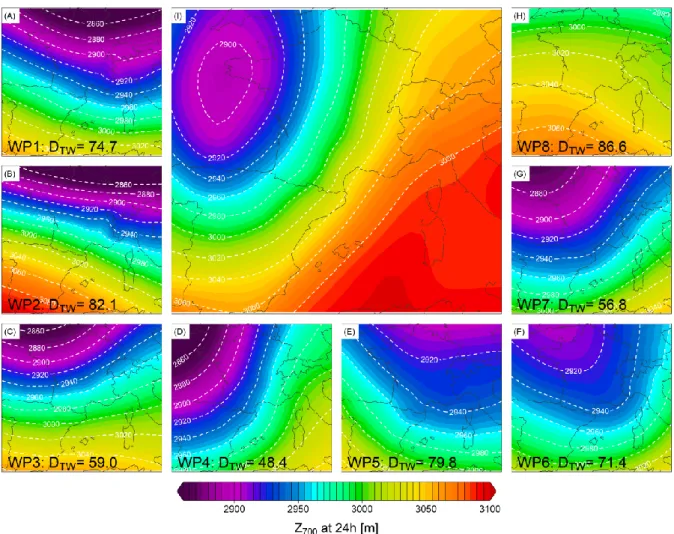
France (-7.50° to 12.75° of longitude and 37.50° to 50.25° of latitude). Figure 1 shows the average Z700
166
field at 24h of each WP, estimated over the 1979-1996 period, and the spatial coverage of the 504 167
ERAi grid points. 168
3.1.2 Classification of the historical period
169
In order to obtain a daily classification for the studied historical period, each past day is assigned to 170
one of the eight WP by computing distances between the synoptic situation of the studied day and 171
each WP. Teweles & Wobus (1954) distances (noted DTW hereafter) are calculated to find the closest
172
WP to each considered day (see Brigode et al., 2013a, 2013b for more details). DTW focuses on air flows
173
since this distance involves gradients of absolute values of geopotential heights (Woodcock, 1980; 174
Obled et al., 2002; Bontron, 2004; Wetterhall et al., 2005, Brigode et al., 2016). The formula for 175
estimating DTW between two synoptic situations (Z1) and (Z2) characterized by geopotential height
176
fields on a gridded domain oriented south-north (index i) and west-east (index j) is : 177 DTW = ∑ |eGi| i,j + ∑ |eG j | i,j ∑ |GLi| i,j + ∑ |GL j| i,j × 100 178
International Journal of Climatology Page 6 on 25 where eG is the difference, around a given grid point, between the Z1 and Z2 geopotential gradients,
179
while GL is the maximum of these two gradients in the direction considered (i or j):
180
|eGi| = |(Z1i,j− Z1i+1,1) − (Z2i,j− Z2i+1,1)|
181
|eGj| = |(Z1i,j− Z1i,j+1) − (Z2i,j− Z2i,j+1)|
182
|GLi| = max(|Z1i,j− Z1i+1,1|, |Z2i,j− Z2i+1,1|)
183
|GLj| = max(|Z1i,j− Z1i,j+1|, |Z2i,j− Z2i,j+1|)
184
DTW ranges from 0 for two identical geopotential fields and 200 for two opposite geopotential fields.
185
The final score between one day and one WP is the sum of four DTW distances: (i) the DTW between the
186
Z700 fields at 0h, (ii) the DTW between the Z1000 fields at 24h, (iii) the DTW between the Z700 fields at 0h
187
and (iv) the DTW between the Z700 fields at 24h. The DTW calculation is illustrated in figure 1, which shows
188
the eight DTW calculated between one particular day (21th September 1992) and the average synoptic
189
situation of the eight French WPs for the Z700 fields at 24h. The minimal DTW is found for the WP4
190
(DTW=48.4). The three other calculations of DTW for that particular day (Z1000 at 0h, Z1000 at 24h and Z700
191
at 0h) are summarized in the table 1. The sum of the four DTW is minimal for the WP4 (DTW=205.5): the
192
21th September 1992 is thus attributed to the WP4. Note that this synoptic situation has generated a
193
considerable amount of precipitation in South-Eastern France, with more than 300 mm of precipitation 194
observed locally that day (Benech et al., 1993), generating a catastrophic and deadly flash flood of the 195
Ouvèze river (Sénési et al., 1996). 196
197
Table 1: DTW distances calculated between the 21th September 1992 synoptic situation and the average
198
synoptic situation of the eight French WPs for the Z1000 and Z700 fields at 0h and at 24h. In this case, the
199
21th September 1992 is finally attributed to the WP4.
200 WP1 WP2 WP3 WP4 WP5 WP6 WP7 WP8 Z1000 at 0h 91.9 101.1 85.3 67.9 95.2 81.1 70.7 96.8 Z1000 at 24h 92.0 91.7 67.6 52.2 89.6 84.1 64.2 99.6 Z700 at 0h 62.5 73.3 49.7 36.9 63.4 63.6 46.1 70.4 Z700 at 24h 74.7 82.1 59.0 48.4 79.8 71.4 56.8 86.6 DTW sums 321.1 348.2 261.6 205.5 328.1 300.3 237.7 353.4 201
International Journal of Climatology Page 7 on 25 202
Figure 1: Comparison between the Z700 synoptic situation of the 21th September 1992 (at 24h, panel I) 203
and the Z700 situation of the eight French WP (panels A to H). The DTW distances calculated between 204
these geopotential fields are given on each panel. 205
206
3.1.3 Meteorological description of the eight French WP
207
The eight French WPs are described in the figures 2.1 and 2.2, in terms of average ERAi Z700 and
208
Z1000 fields at 0h, E-OBS regional precipitation pattern and seasonal frequencies, calculated over the
209
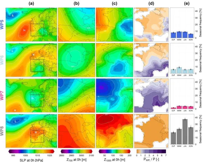
1979-2004 period. The eight WP can be grouped in terms of their general atmospheric flow direction 210
(cf. column (a) of the figures 2.1 and 2.2, showing average SLP for each WP): 211
WP1 (Atlantic Wave), WP2 (Steady Oceanic) and WP3 (Southwest Circulation) correspond to 212
westerly oceanic circulation, grouping days particularly rainy over the Alps, the Northwestern 213
part of France and the Western part of France, respectively. The WP2 is one of the most frequent 214
over the year, especially during the winter season. 215
WP4 (South Circulation), WP6 (East Return) and WP7 (Central Depression) correspond to 216
Mediterranean circulations, grouping days particularly rainy over the Southeastern part of 217
France. WP6 and WP7 days are relatively rarely observed. 218
The WP5 (Northeast Circulation) corresponds to continental circulations, grouping days not 219
particularly rainy over France. 220
International Journal of Climatology Page 8 on 25 Finally, the WP8 (Anticyclonic) corresponds to high pressure situations and thus groups non-221
rainy days. This French WP is the most frequent, especially in summer. 222
223
224
Figure 2.1: Description of the WP1 to WP4: (a) average ERAi SLP at 0h, (b) average ERAi Z700 at 0h, (c) 225
average ERAi Z1000 at 0h, (d) ratio between the E-OBS mean precipitation amounts and the general 226
precipitation amount (considering all WP) and (e) seasonal frequency of the WP, estimated over the 227
1979-2004 period. 228
International Journal of Climatology Page 9 on 25 229
Figure 2.2: Description of the WP5 to WP8: (a) average ERAi SLP at 0h, (b) average ERAi Z700 at 0h, (c) 230
average ERAi Z1000 at 0h, (d) ratio between the E-OBS mean precipitation amounts and the general 231
precipitation amount (considering all WP) and (e) seasonal frequency of the WP, estimated over the 232
1979-2004 period. 233
234
3.2 Classification of the daily GCM outputs
235
The classification of the geopotential height fields simulated by the GCM has been done with the same 236
methodology, i.e. by calculating DTW between each simulated day (characterized by four synoptic
237
situations: Z1000 at 0h, Z1000 at 24h, Z700 at 0h and Z700 at 24h) and the ERAi average situations of the
238
eight French WP (also being characterized by four synoptic situations). The sum of the four DTW is
239
calculated for each simulated day and each WP, and the WP with the minimal DTW sum is attributed to
240
the studied day. 241
3.3 Geopotential height bias correction methods
242
While most of the studies on the GCM WP simulation used uncorrected GCM outputs, it is 243
noteworthy that Demuzere et al. (2009) and Lorenzo et al. (2011) found better performances of GCM 244
in terms of frequencies if the SLP fields used for the classification were bias-corrected before the 245
classification procedure. Thus, the need for bias correction of GCM geopotential height fields before 246
performing WP classification will be tested in this paper, by considering different bias correction 247
methods. 248
International Journal of Climatology Page 10 on 25 DTW distance values have been firstly computed without correcting the GCM geopotential height
249
fields. The WP frequencies obtained by using these uncorrected GCM outputs are named D0 hereafter. 250
Then, four different bias correction methods have been applied to the GCM outputs: 251
1. A spatially homogeneous correction of the geopotential height average values and standard 252
deviations. The outputs of this bias correction method are named D1 hereafter. Note that since 253
DTW are estimated by considering synoptic circulation gradients, a spatially homogeneous
254
correction of average values only is useless: lowering or rising the mean geopotential height 255
fields has no effect on the DTW values.
256
2. A spatially nonhomogeneous correction of the average values. The outputs of this bias 257
correction method are named D2 hereafter. 258
3. A spatially nonhomogeneous correction of the geopotential height average values and standard 259
deviations. The outputs of this bias correction method are named D3 hereafter. 260
4. A spatially nonhomogeneous correction of the monthly average values and standard deviations. 261
The outputs of this bias correction method are named D4 hereafter. 262
To summarize, each GCM output is considered five times: firstly without any bias correction method 263
(outputs named D0) and then after application of the D1, D2, D3 and D4 bias correction methods. 264
3.4 Seasonal WP frequencies and frequency variability
265
Seasonal frequencies of the eight French WP have been estimated over the 25-year historical period 266
(01/03/1979-29/02/2004) and over 68 25-year periods extracted from the future RCP simulations 267
(2006-2031, 2007-2032, …, 2073-2098). Four 3-month seasons have been defined: the autumn season 268
(September, October and November, noted SON hereafter), the winter season (December, January 269
and February, noted DJF hereafter) the spring season (March, April and May, noted MAM hereafter) 270
and the summer season (June, July and August, noted JJA hereafter). For each season and each WP, 271
frequencies are defined as the percentage of days belonging to the considered WP. The reference 272
observed seasonal frequencies of the eight WP are the seasonal frequencies represented in column (e) 273
of figures 2.1 and 2.2. 274
In order to quantify the WP frequency variability within a time period, a non-parametric bootstrap 275
resampling has been performed. Thus, for each 25-year time period considered, 100 samples of 15 276
randomly chosen years are constructed. Note that no replacements are allowed within this bootstrap 277
resampling, and thus one particular year cannot be resampled twice. These 100 samples are then used 278
to quantify the variability of the frequency by measuring the 90% confidence interval. The dispersion 279
of observed WP frequencies are shown in figures 2.1 and 2.2 for the 1979-2004 period. The observed 280
variability of the seasonal frequencies is limited, the highest variability is observed for the WP2, WP4 281
and WP8. For example, the summer frequency of WP8 ranges between 33.2% and 38.8%. 282
International Journal of Climatology Page 11 on 25
4 RESULTS
284
4.1 GCM simulations of WP average Z
1000and Z
700285
The GCM ensemble outputs have been firstly evaluated in terms of the simulation of the average 286
Z700 and Z1000 fields for the eight WP, over the 1979-2004 period. Figure 3 summarizes the spatial
287
variability of the Z1000 and Z700 bias, calculated for each WP as the difference between the GCM
288
ensemble mean fields and the average ERAi fields (presented in the figures 2.1 and 2.2). For Z700, the
289
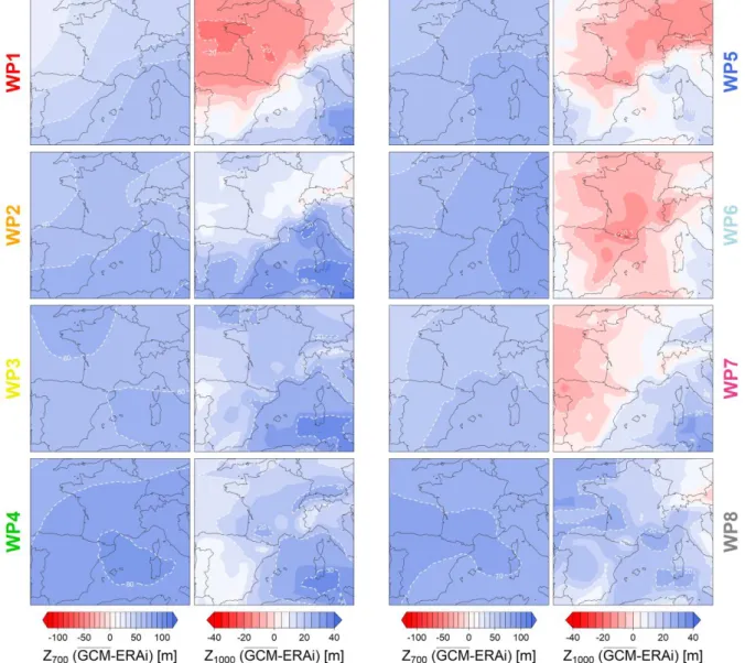
GCM ensemble appears to overestimate the geopotential heights for the eight WP. The spatial 290
distributions of theses biases reveal a slighter bias over northwestern France (Atlantic Sea). The spatial 291
distribution of Z1000 bias changes with WP. For WP1, WP5 and WP7, the GCM ensemble tends to
292
underestimate the Z1000 values over northwestern France and to overestimate the Z1000 values over the
293
southeastern part of the studied region. For the WP6, the Z1000 values are slightly underestimated over
294
the entire studied region. For the other WP (WP2, WP3, WP4 and WP6), the GCM ensemble tends 295
generally to overestimate the Z1000 values over the studied region. The spatial variability of biases
296
justified the use of bias correction method that are spatially (D2 to D4) nonhomogeneous. 297
International Journal of Climatology Page 12 on 25 299
Figure 3: Z700 and Z1000 geopotential bias calculated for each WP as the difference between GCM 300
ensemble mean and ERAi geopotential height fields. 301
302
4.2 Historical seasonal WP frequencies simulated by the GCM ensemble
303
The GCM ensemble has then been evaluated in terms of simulating historical WP frequencies for 304
the four different seasons considered. Figure 4 presents the observed (ERAi) seasonal WP frequencies 305
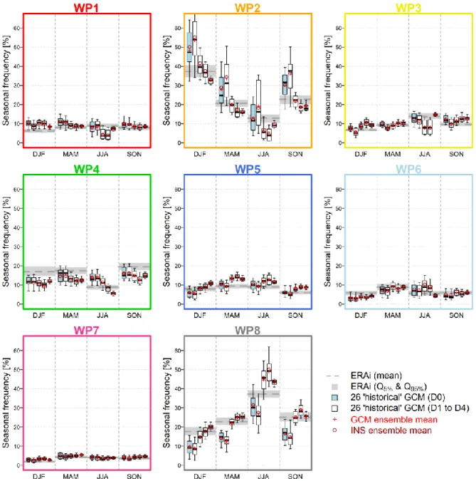
estimated over the 1979-2004 period and the WP frequencies simulated by the GCM ensemble 306
(uncorrected and corrected). The seasonal variability of the WP frequencies are generally well 307
simulated by the uncorrected GCM (expect for the WP4). Nevertheless, the frequencies of the two 308
most frequent WP (WP2 and WP8) are poorly simulated, with WP2 frequencies being strongly 309
overestimated and WP8 strongly underestimated. Moreover, the dispersion of the GCM ensemble is 310
large for these two WP as well as for the WP4. The impact of the different bias correction methods on 311
the historical WP frequencies is not straightforward and needs further investigations. 312
International Journal of Climatology Page 13 on 25 313
Figure 4: Seasonal WP frequencies estimated over the 1979-2004 period. The grey rectangles present
314
the observed (ERAi) WP frequencies. The boxplots are constructed with the WP frequencies simulated 315
by the GCM ensembles (GCM and INS) without bias correction (blue boxplots) and with bias corrections 316
(white boxplots, D1 to D4). 317
318
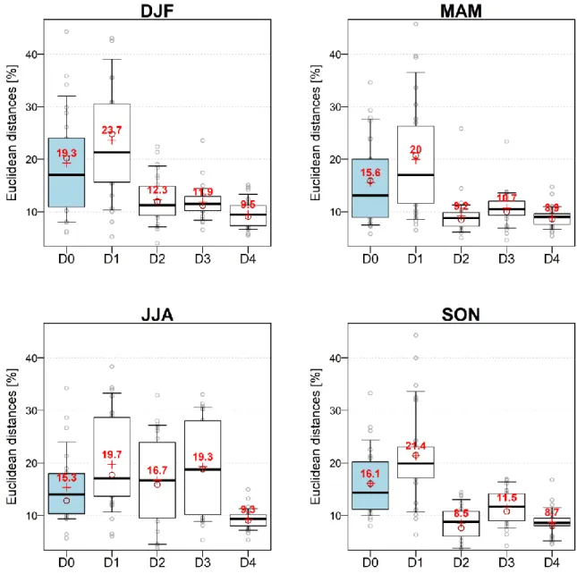
Figure 5 presents the distribution of Euclidean distances calculated, for each season and each bias 319
correction method, between the vector of the 8 observed WP frequencies and the 26 vectors of 8 320
simulated WP frequencies. When no bias correction is applied (D0 method), the GCM ensemble is 321
slightly less performant for DJF season (average distance around 19%) than for other seasons (average 322
distance around 15.5%). The application of the D1 bias correction method (spatially homogeneous 323
correction of the geopotential height standard deviations) appears to degrade the performance of the 324
GCM ensemble in terms of seasonal WP frequencies. Nevertheless, the application of the D2 to D4 325
correction methods (all spatially inhomogeneous correction methods) improves the GCM ensemble 326
performances for the DJF, MAM and SON seasons. For the JJA season, only the D4 bias correction 327
International Journal of Climatology Page 14 on 25 method improves the performance of the WP frequency simulation. Overall, the D4 bias correction 328
method (only method implying a spatial and temporal nonhomogenous correction) has the best 329
performances in terms of simulation of the ERAi WP frequencies on the historical period. 330
331
332
Figure 5: Distributions of seasonal Euclidean distances calculated, for each season and each bias
333
correction method, between the vector of 8 observed WP frequencies and the 26 vectors of 8 simulated 334
(GCM) WP frequencies over the 1979-2004 period. The blue boxplots are WP frequencies obtained 335
without bias correction, and the white ones are obtained when the bias correction D1 to D4 are applied. 336
Red values are mean values of Euclidean distances between WP frequency vectors and grey points are 337
individual GCM distances. 338
International Journal of Climatology Page 15 on 25
4.3 Future evolutions of seasonal WP frequencies
340
In this section, the changes of WP frequencies simulated by the GCM ensemble are calculated. 341
Regarding the performances obtained by the four different bias correction methods tested (see 342
Section 4.2), only the best method (D4) has been considered for the estimation of future WP 343
frequencies. Thus, future frequencies are calculated with both uncorrected GCM outputs (D0) and 344
GCM outputs corrected with the D4 method. 345
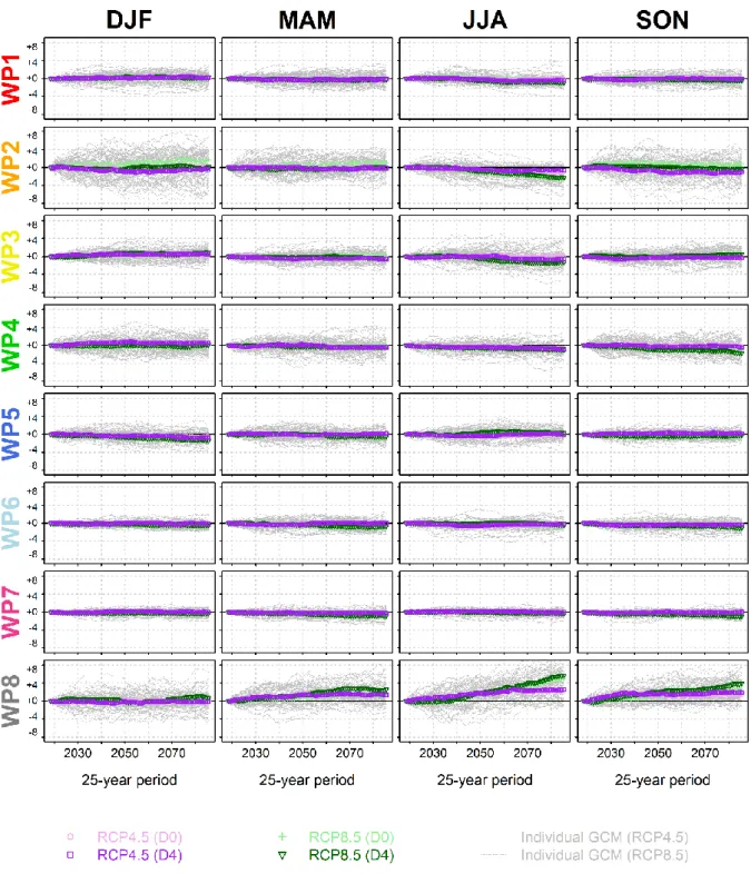
Figure 6 presents the mean seasonal frequency evolutions simulated by the GCM ensemble, 346
considering both RCP4.5 and RCP8.5 emission scenarios and both GCM outputs without bias correction 347
and GCM outputs corrected with the D4 method. None particular temporal evolutions throughout 348
seasons are simulated for WP1, WP5, WP6 and WP7. WP3 and WP4 appear to be slightly less frequent 349
at the end of the century during JJA and SON seasons, respectively. These slight decreases seem to be 350
more pronounced when considering the RCP8.5 simulations. WP2 and WP8 are the two WP with the 351
most pronounced seasonal changes and are in opposition. Overall, WP2 is slightly less frequent (but 352
its frequency evolution depends on the RCP outputs considered), while WP8 is highly more frequent. 353
These conjoint evolutions are particularly notable for the JJA season. For this season, WP8 frequency 354
is constantly increasing with time for RCP8.5 outputs, while the frequency increase is stopped around 355
the 2060 years for RCP4.5. Oppositely, the WP2 frequency decrease for the same season is stronger 356
when considering RCP8.5 outputs. For the SON season, a strong increase of WP8 is also notable, while 357
a slight decrease of WP4 and WP2 frequencies is found (expect for uncorrected RCP8.5 outputs). For 358
the DJF and MAM seasons, the WP8 appears to be also more frequent, while no particular frequency 359
evolution is found for WP2. 360
International Journal of Climatology Page 16 on 25 362
Figure 6: Seasonal WP frequency changes (in %) estimated with the GCM ensemble over 68 consecutive
363
25-year periods, considering RCP4.5 and RCP8.5 simulations, with no bias correction (D0) and with the 364
D4 bias correction method. Changes are relative to the WP frequencies simulated by the GCM ensemble 365
over the first 25-year period (2006-2031). Grey lines are individual GCM WP frequency changes. 366
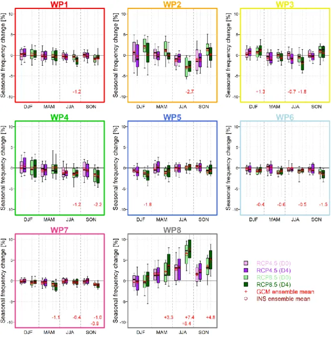
International Journal of Climatology Page 17 on 25 Figure 7 summarizes the frequency changes calculated between the 2006-2031 period and the 368
2073-2098 period. A Student's t-Test has been performed for highlighting the significant changes of 369
mean seasonal frequency (p-value < 5%). The dispersion of simulated changes is different depending 370
on the WP, with larger dispersion for WP2, WP4 and WP8 frequencies. WP1 frequency appears to only 371
slightly decrease in JJA months for the RCP8.5 simulations (-1.2%, 95% of the GCM ensemble simulating 372
a decrease), when geopotential height bias are corrected with the D4 method. For WP2, the simulated 373
changes are highly dependent on the season and on the application of a bias correction method. After 374
bias correction, no clear frequency changes are obtained when considering RCP4.5 outputs. 375
Nevertheless, the RCP8.5 outputs show a significant decrease of WP2 frequency for the JJA season 376
with the bias correction method applied (-2.7%, 90% of the GCM ensemble simulating a decrease). 377
WP3 appears to be slightly more frequent for DJF (significant increase of +1.3%, 75% of the GCM 378
ensemble simulating an increase, with D4 correction method), while being less frequent for JJA season 379
(significant decrease of -1.8%, 81% of the GCM ensemble simulating a decrease, with D4 correction 380
method), for the RCP8.5 simulations. The summer decrease of the WP3 frequency is also found in the 381
bias-corrected RCP4.5 simulations (significant decrease of -0.7%, 58% of the GCM ensemble simulating 382
a decrease). WP4 are significantly less frequent in JJA season RCP8.5 (-1.2%, 81% of the GCM ensemble 383
simulating a decrease) scenarios and in SON season for bias corrected RCP8.5 (-2.2%) scenarios. A 384
significant decrease of -1.8% in the DJF season is found for WP5 for the bias corrected RCP8.5 385
simulations (decrease simulated by 81% of the GCM ensemble), while no significant changes are found 386
for the other seasons and outputs. The bias corrected RCP8.5 outputs show significant less WP6 days 387
for the different seasons, with a stronger decrease for the SON season (-1.5%, 95% of the GCM 388
ensemble simulating a decrease).The WP7 is slightly less frequent for MAM, JJA and SON seasons, 389
especially when considering RCP8.5 and bias-corrected outputs (-1.1%, -0.4% and -1.0% for these three 390
seasons, decreases simulated by 81%, 67% and 81% of the GCM ensemble, respectively). Finally, the 391
WP8 frequency is significantly increasing for MAM, JJA and SON seasons. These increases are stronger 392
when considering bias corrected RCP8.5 outputs (+3.3%, +7.4% and +4.8%, increases simulated by 393
81%, 95% and 90% of the GCM ensemble respectively). 394
The summer (JJA) Z700 values simulated by the GCM ensemble is increasing with time over the
395
studied domain. The GCM ensemble mean is 3137 m around 2018 and is 3183 m around 2085, 396
considering the RCP8.5 scenario. This increase seems to be correlated with the decrease of the WP2 397
summer frequency and with the increase of the WP8 summer frequency (results not shown). 398
Nevertheless, the WP classification was performed using the Teweles & Wobus (1954) distance (DTW),
399
metric calculated with the geopotential height gradients and not with the absolute values of the 400
geopotential heights. Thus, the temporal increase of the geopotential height absolute values is not 401
influencing the DTW calculation and the simulated increase (decrease) of the seasonal WP8 (WP2)
402
frequency are thus due to changes in general circulation over the studied domain and not due to the 403
global increase of surface pressure in future climate. 404
International Journal of Climatology Page 18 on 25 406
Figure 7: Seasonal WP frequency changes estimated with the GCM ensemble between 2073-2098
407
period and 2006-2031 period, considering RCP4.5 and RCP8.5 simulations, with no bias correction (D0) 408
and with the D4 bias correction. The significant changes of mean WP frequency are printed in red color 409
and expressed as percentage of frequency change. 410
International Journal of Climatology Page 19 on 25
5 DISCUSSION AND CONCLUSION
411
An ensemble of 26 GCM used within the fifth Coupled Model Intercomparison Project (CMIP5) have 412
been analyzed in order firstly to test its ability to reproduce observed seasonal geopotential height 413
climatology over Western Europe, secondly to test its ability to reproduce the seasonal frequencies of 414
eight French WPs previously defined (Garavaglia et al., 2010) and finally to estimate the future 415
seasonal WP frequencies. 416
Firstly, biases of simulated Z1000 and Z700 have been quantified over Western Europe for the
417
historical period (here 1979-2004), relatively to the ERAi reanalysis. For Z1000, the GCM ensemble biases
418
have both a strong spatial variability and seasonal variability. For example, the GCM ensemble tends 419
to underestimate the geopotential heights at the highest latitudes of the Western Europe in DJF and 420
MAM seasons, while it tends to overestimate geopotential heights at the same latitudes for the JJA 421
and SON seasons. For Z700, the GCM ensemble tends to overestimate the geopotential heights for the
422
four seasons, with a slighter bias over northern latitudes. These spatial and seasonal variabilities of 423
geopotential biases could advocate the use of spatially and seasonally inhomogeneous bias correction 424
methods on the geopotential height outputs. 425
Secondly, the ability of the GCM ensemble to reproduce historical WP frequencies has been 426
quantified and revealed that the seasonal variability of the WP frequencies are generally well 427
simulated by the uncorrected GCM ensemble (expect for the WP4), with a slightly worse performance 428
obtained for the DJF season. Nevertheless, the frequencies of the two most frequent WP (WP2 and 429
WP8) are poorly simulated by the ensemble, with WP2 frequencies being strongly overestimated and 430
WP8 strongly underestimated. Similar results have been obtained by Santos et al. (2016) by looking at 431
WP frequencies simulated by an ensemble of 22 GCM over Western Europe and showing the 432
overestimation by this other ensemble of the frequency of WP associated with zonal airflow. The use 433
of four different bias correction methods showed that the application of a spatially and temporally 434
nonhomogeneous correction of geopotential height fields (here the correction named D4) improved 435
significantly the simulation of WP frequencies for the four seasons. 436
Finally, the evolution of the WP frequencies over the next century has been quantified, considering 437
two emission scenarios (RCP4.5 and RCP8.5) and considering one bias correction method (D4) and no 438
bias correction. The WP2, WP4 and WP8 have more pronounced seasonal changes, with WP2 and WP4 439
being less frequent in JJA and SON seasons, respectively, while WP8 being more frequent over MAM, 440
JJA and SON season. The frequency changes calculated are higher for RCP8.5 simulations than for 441
RCP4.5. Moreover, the temporal evolution of the WP frequencies appears to be constant over time for 442
RCP8.5, while the evolution stops around the year 2060 for the RCP4.5 scenario. The use of a bias 443
correction method is important in this context, since the significant mean changes of WP frequencies 444
are all obtained with bias-corrected outputs (expect the increase of WP8 summer frequency). 445
Nevertheless, the analysis of the temporal evolution of WP frequencies (figure 6) and the distribution 446
of simulated frequency changes (figure 7) showed that the bias-correction method used (D4) is not 447
changing the sign of the mean frequency changes compared to the uncorrected GCM outputs. Note 448
that the use of three other bias correction methods (D1 to D3) leads to the same change signs for the 449
different WP and seasons (results not shown). 450
International Journal of Climatology Page 20 on 25 The strong simulated frequency evolution of WP2 and WP8 is an interesting result, which predicts 452
the climate to be drier with time for France. Thus, WP2 (western oceanic circulation), grouping rainy 453
days over the northern France region, is simulated as less frequent in future summers, while WP8 454
(Anticyclonic situations), which groups non-rainy days over France, is simulated as more frequent in 455
future summers. These evolutions could have significant impacts on French low flows, since Giuntoli 456
et al. (2013) recently highlighted strong correlations between these WP frequency and drought 457
severity over France. An increase of the frequency of non-rainy WP is also found in the 22 GCM 458
ensemble studied by Santos et al. (2016) when considering RCP8.5 outputs. 459
The bias of CMIP5 GCM in terms of the simulation of the eight French WP frequencies rises several 460
questions, firstly about the WP classification methodology considered here. Thus, Vrac et al. (2007) 461
showed that the WP classification method used has an impact on the identified patterns, and also that 462
the choice of a given reanalysis as reference could lead to different WP classifications. Applying 463
different classification methods on the same GCM ensemble and considering other reanalysis as 464
reference would be an interesting perspective, in order to see if similar French WP are identified. In 465
addition, the applied methodology assumes that only the WP frequencies are changing in the future, 466
while WP structures are considered as constant in time. Küttel et al. (2010) thus highlighted large 467
changes within type variations for European WP. The application of the methodology developed by 468
Cattiaux et al. (2012) could be an interesting perspective in order to fully split the part of changes 469
explained by WP frequencies and the part explained by WP structures, for example. 470
The second question to be raised is the spatial domain considered here for the definition of the WP 471
classification and, consequently, for studying WP frequencies simulated by the GCM ensemble. This 472
domain is rather small (-7.50° to 12.75° of longitude and 37.50° to 50.25° of latitude), thus concerning 473
only a limited grid points for the GCM characterized by a limited atmospheric horizontal resolution. If 474
the WP identified at this spatial scale have relevant characteristics in terms of spatial distribution of 475
surface variables such as precipitation over France, it is possible that the horizontal resolution of GCM 476
are too large for allowing them to identify such regional patterns. Nuissier et al. (2011), with a rather 477
similar objective of determining WP leading to heavy precipitation events over southern France, used 478
a larger spatial domain for the WP classification (-24° to +39° of longitude and 25.5° to 63° for latitude). 479
Thus, trying to define French WP over a larger spatial domain is an interesting perspective, in order to 480
quantify the future WP frequencies. The use of Regional Climate Model (RCM) could also be an 481
interesting perspective, even though recent work questioned the ability of RCM to reproduce the daily 482
weather regimes (e.g. Lucas-Picher et al., 2016). 483
Finally, the use of spatially nonhomogeneous bias correction methods for geopotential height fields 484
is questionable, since these corrections change the simulated circulation patterns, transforming the 485
GCM outputs in order to be more similar to the reference ones. Moreover, the biases quantified over 486
the historical period have to be assumed as being stationary over time in order to be applied over the 487
future time period considered, which is a strong hypothesis. 488
489
The ultimate goal of this work was to use simulated future frequencies of particular WPs - known 490
to potentially leading to heavy precipitation events (and then extreme floods) - in order to discuss 491
future precipitation (floods) frequency. Within this framework, only the frequency of future rainfall 492
events is studied, thus splitting frequency (related to circulation dynamic) and intensity (related to 493
thermo-dynamic parameters) of such events. Nevertheless, recent studies highlighted that both 494
International Journal of Climatology Page 21 on 25 frequency and intensity have to be studied for discussing future extreme precipitation (e.g. Hertig et 495
al., 2013; Blenkinsop et al., 2015) or climate extreme event attribution (e.g. Trenberth et al., 2015). 496
Finally, another interesting future work would be to study the potential shift of WP persistence over 497
the same region and with the same GCM ensemble, since the persistence of rainy or non-rainy WPs is 498
a good indicator for flood or drought frequency and intensity. 499
500
6 ACKNOWLEDGEMENTS
501
We acknowledge the World Climate Research Programme's Working Group on Coupled Modelling, 502
which is responsible for CMIP, and we thank the climate modeling groups (listed in table S1 of this 503
paper) for producing and making available their model output. For CMIP the U.S. Department of 504
Energy's Program for Climate Model Diagnosis and Intercomparison provides coordinating support and 505
led development of software infrastructure in partnership with the Global Organization for Earth 506
System Science Portals. We also acknowledge the E-OBS dataset from the EU-FP6 project ENSEMBLES 507
(http://ensembles-eu.metoffice.com) and the data providers in the ECA&D project 508
(http://www.ecad.eu). The authors thank the two reviewers, who provided constructive comments on 509
an earlier version of the manuscript, which helped clarify the text. 510
511
7 BIBLIOGRAPHY
512
Anagnostopoulou C, Tolika K, Maheras P, Kutiel H, Flocas HA. 2008. Performance of the general 513
circulation HadAM3P model in simulating circulation types over the Mediterranean region. 514
International Journal of Climatology 28(2): 185–203. DOI: 10.1002/joc.1521. 515
Belleflamme A, Fettweis X, Erpicum M. 2014. Do global warming-induced circulation pattern changes 516
affect temperature and precipitation over Europe during summer? International Journal of Climatology 517
35(7): 1484–1499. DOI: 10.1002/joc.4070. 518
Belleflamme A, Fettweis X, Lang C, Erpicum M. 2013. Current and future atmospheric circulation at 500 519
hPa over Greenland simulated by the CMIP3 and CMIP5 global models. Climate Dynamics 41(7–8): 520
2061–2080. DOI: 10.1007/s00382-012-1538-2. 521
Benech B, Brunet H, Jacq V, Payen M, Rivrain J-C, Santurette P. 1993. La catastrophe de Vaison-La-522
Romaine et les violentes précipitations de septembre 1992: aspects météorologiques. La Météorologie 523
(1): 72–90. 524
Blenkinsop S, Chan SC, Kendon EJ, Roberts NM, Fowler HJ. 2015. Temperature influences on intense 525
UK hourly precipitation and dependency on large-scale circulation. Environmental Research Letters 526
10(5): 054021. DOI: 10.1088/1748-9326/10/5/054021. 527
Boé J, Terray L. 2008. A Weather-Type Approach to Analyzing Winter Precipitation in France: 528
Twentieth-Century Trends and the Role of Anthropogenic Forcing. Journal of Climate 21(13): 3118– 529
3133. DOI: 10.1175/2007JCLI1796.1. 530
International Journal of Climatology Page 22 on 25 Bontron G. 2004. Prévision quantitative des précipitations: adaptation probabiliste par recherche 531
d’analogues. Utilisation des ré-analyses NCEP/NCAR et application aux précipitations du Sud-Est de la 532
France. Institut Polytechnique de Grenoble, PhD thesis, 276 pp. 533
Brigode P, Brissette F, Nicault A, Perreault L, Kuentz A, Mathevet T, Gailhard J. 2016. Streamflow 534
variability over the 1881–2011 period in northern Québec: comparison of hydrological reconstructions 535
based on tree rings and geopotential height field reanalysis. Climate of the Past 12(9): 1785–1804. DOI: 536
10.5194/cp-12-1785-2016. 537
Brigode, P, Bernardara P, Gailhard J, Garavaglia F, Ribstein P, Merz R. 2013a. Optimization of the 538
Geopotential Heights Information Used in a Rainfall-Based Weather Patterns Classification over 539
Austria. International Journal of Climatology 33(6): 1563–1573. DOI:10.1002/joc.3535. 540
Brigode P, Mićović Z, Bernardara P, Paquet E, Garavaglia F, Gailhard J, Ribstein P. 2013b. Linking ENSO 541
and heavy rainfall events over coastal British Columbia through a weather pattern classification. 542
Hydrology and Earth System Sciences 17(4): 1455–1473. DOI: 10.5194/hess-17-1455-2013. 543
Cassano JJ, Uotila P, Lynch A. 2006. Changes in synoptic weather patterns in the polar regions in the 544
twentieth and twenty-first centuries, part 1: Arctic. International Journal of Climatology 26(8): 1027– 545
1049. DOI: 10.1002/joc.1306. 546
Cassou C, Terray L, Hurrell JW, Deser C. 2004. North Atlantic Winter Climate Regimes: Spatial 547
Asymmetry, Stationarity with Time, and Oceanic Forcing. Journal of Climate 17(5): 1055–1068. DOI: 548
10.1175/1520-0442(2004)017<1055:NAWCRS>2.0.CO;2. 549
Cassou C, Terray L, Phillips AS. 2005. Tropical Atlantic Influence on European Heat Waves. Journal of 550
Climate 18(15): 2805–2811. DOI: 10.1175/JCLI3506.1. 551
Cattiaux J, Douville H, Ribes A, Chauvin F, Plante C. 2012. Towards a better understanding of changes 552
in wintertime cold extremes over Europe: a pilot study with CNRM and IPSL atmospheric models. 553
Climate Dynamics 40: 2433. DOI: 10.1007/s00382-012-1436-7. 554
Corti S, Molteni F, Palmer TN. 1999. Signature of recent climate change in frequencies of natural 555
atmospheric circulation regimes. Nature 398(6730): 799–802. DOI: 10.1038/19745. 556
Covey C, AchutaRao KM, Cubasch U, Jones P, Lambert SJ, Mann ME, Phillips TJ, Taylor KE. 2003. An 557
overview of results from the Coupled Model Intercomparison Project. Global and Planetary Change 558
37(1–2): 103–133. DOI: 10.1016/S0921-8181(02)00193-5. 559
Dee DP, Uppala SM, Simmons AJ, Berrisford P, Poli P, Kobayashi S, Andrae U, Balmaseda MA, Balsamo 560
G, Bauer P, Bechtold P, Beljaars ACM, van de Berg L, Bidlot J, Bormann N, Delsol C, Dragani R, Fuentes 561
M, Geer AJ, Haimberger L, Healy SB, Hersbach H, Hólm EV, Isaksen L, Kållberg P, Köhler M, Matricardi 562
M, McNally AP, Monge-Sanz BM, Morcrette J-J, Park B-K, Peubey C, de Rosnay P, Tavolato C, Thépaut 563
J-N, Vitart F. 2011. The ERA-Interim reanalysis: configuration and performance of the data assimilation 564
system. Quarterly Journal of the Royal Meteorological Society 137(656): 553–597. DOI: 10.1002/qj.828. 565
Demuzere M, Werner M, van Lipzig NPM, Roeckner E. 2009. An analysis of present and future ECHAM5 566
pressure fields using a classification of circulation patterns. International Journal of Climatology 29(12): 567
1796–1810. DOI: 10.1002/joc.1821. 568
Dunn-Sigouin E, Son S-W. 2013. Northern Hemisphere blocking frequency and duration in the CMIP5 569
models. Journal of Geophysical Research 118(3): 1179–1188. DOI: 10.1002/jgrd.50143. 570
International Journal of Climatology Page 23 on 25 Garavaglia F, Gailhard J, Paquet E, Lang M, Garçon R, Bernardara P. 2010. Introducing a rainfall 571
compound distribution model based on weather patterns sub-sampling. Hydrology and Earth System 572
Sciences 14(6): 951–964. DOI: 10.5194/hess-14-951-2010. 573
Garavaglia F, Lang M, Paquet E, Gailhard J, Garçon R, Renard B. 2011. Reliability and robustness of 574
rainfall compound distribution model based on weather pattern sub-sampling. Hydrology and Earth 575
System Sciences 15(2): 519–532. DOI: 10.5194/hess-15-519-2011. 576
Gillett NP, Zwiers FW, Weaver AJ, Stott PA. 2003. Detection of human influence on sea-level pressure. 577
Nature 422(6929): 292–294. 578
Giuntoli I, Renard B, Vidal J-P, Bard A. 2013. Low flows in France and their relationship to large-scale 579
climate indices. Journal of Hydrology 482: 105–118. DOI: 10.1016/j.jhydrol.2012.12.038. 580
Hall A. 2014. Projecting regional change. Science 346(6216): 1461–1462. DOI: 581
10.1126/science.aaa0629. 582
Handorf D, Dethloff K. 2012. How well do state-of-the-art atmosphere-ocean general circulation 583
models reproduce atmospheric teleconnection patterns? Tellus A 64(0). DOI: 584
10.3402/tellusa.v64i0.19777. 585
Haylock MR, Hofstra N, Tank AMG., Klok EJ, Jones PD, New M. 2008. A European daily high-resolution 586
gridded data set of surface temperature and precipitation for 1950–2006. Journal of Geophysical 587
Research 113(D20): D20119. DOI: 10.1029/2008JD010201. 588
Hertig E, Jacobeit J. 2014. Variability of weather regimes in the North Atlantic-European area: past and 589
future. Atmospheric Science Letters 15(4): 314–320. DOI: 10.1002/asl2.505. 590
Hertig E, Seubert S, Paxian A, Vogt G, Paeth H, Jacobeit J. 2013. Statistical modelling of extreme 591
precipitation indices for the Mediterranean area under future climate change. International Journal of 592
Climatology 34(4): 1132–1156. DOI: 10.1002/joc.3751. 593
Hsu CJ, Zwiers F. 2001. Climate change in recurrent regimes and modes of northern hemisphere 594
atmospheric variability. Journal of Geophysical Research 106(D17): 20145–20159. DOI: 595
10.1029/2001JD900229. 596
Huth R, Beck C, Philipp A, Demuzere M, Ustrnul Z, Cahynová M, Kyselý J, Tveito OE. 2008. Classifications 597
of Atmospheric Circulation Patterns. Annals of the New York Academy of Sciences 1146(1): 105–152. 598
DOI: 10.1196/annals.1446.019. 599
Küttel M, Luterbacher J, Wanner H. 2010. Multidecadal changes in winter circulation-climate 600
relationship in Europe: frequency variations, within-type modifications, and long-term trends. Climate 601
Dynamics 36(5–6): 957–972. DOI: 10.1007/s00382-009-0737-y. 602
Lorenzo MN, Ramos AM, Taboada JJ, Gimeno L. 2011. Changes in Present and Future Circulation Types 603
Frequency in Northwest Iberian Peninsula. PLoS ONE 6(1). DOI: 10.1371/journal.pone.0016201. 604
Lucas-Picher P, Cattiaux J, Bougie A, Laprise R. 2016. How does large-scale nudging in a regional climate 605
model contribute to improving the simulation of weather regimes and seasonal extremes over North 606
America? Climate Dynamics 46(3–4): 929–948. DOI: 10.1007/s00382-015-2623-0. 607
International Journal of Climatology Page 24 on 25 McKendry IG, Stahl K, Moore RD. 2006. Synoptic sea-level pressure patterns generated by a general 608
circulation model: comparison with types derived from NCEP/NCAR re-analysis and implications for 609
downscaling. International Journal of Climatology 26(12): 1727–1736. DOI: 10.1002/joc.1337. 610
Michelangeli P-A, Vautard R, Legras B. 1995. Weather Regimes: Recurrence and Quasi Stationarity. 611
Journal of Atmospheric Sciences 52: 1237–1256. DOI: 10.1175/1520-612
0469(1995)052<1237:WRRAQS>2.0.CO;2. 613
Moss RH, Edmonds JA, Hibbard KA, Manning MR, Rose SK, Vuuren DP van, Carter TR, Emori S, Kainuma 614
M, Kram T, Meehl GA, Mitchell JFB, Nakicenovic N, Riahi K, Smith SJ, Stouffer RJ, Thomson AM, Weyant 615
JP, Wilbanks TJ. 2010. The next generation of scenarios for climate change research and assessment. 616
Nature 463(7282): 747–756. DOI: 10.1038/nature08823. 617
Murawski A, Bürger G, Vorogushyn S, Merz B. 2016. Can local climate variability be explained by 618
weather patterns? A multi-station evaluation for the Rhine basin. Hydrology and Earth System Sciences 619
20(10): 4283–4306. DOI: 10.5194/hess-20-4283-2016. 620
Nied M, Pardowitz T, Nissen K, Ulbrich U, Hundecha Y, Merz B. 2014. On the relationship between 621
hydro-meteorological patterns and flood types. Journal of Hydrology 519: 3249–3262. DOI: 622
10.1016/j.jhydrol.2014.09.089. 623
Nuissier O, Joly B, Joly A, Ducrocq V, Arbogast P. 2011. A statistical downscaling to identify the large-624
scale circulation patterns associated with heavy precipitation events over southern France. Quarterly 625
Journal of the Royal Meteorological Society 137(660): 1812–1827. DOI: 10.1002/qj.866. 626
Obled C, Bontron G, Garçon R. 2002. Quantitative precipitation forecasts: a statistical adaptation of 627
model outputs through an analogues sorting approach. Atmospheric Research 63(3–4): 303–324. DOI: 628
10.1016/S0169-8095(02)00038-8. 629
Pastor MA, Casado MJ. 2012. Use of circulation types classifications to evaluate AR4 climate models 630
over the Euro-Atlantic region. Climate Dynamics 39(7–8): 2059–2077. DOI: 10.1007/s00382-012-1449-631
2. 632
Philipp A, Della-Marta PM, Jacobeit J, Fereday DR, Jones PD, Moberg A, Wanner H. 2007. Long-Term 633
Variability of Daily North Atlantic–European Pressure Patterns since 1850 Classified by Simulated 634
Annealing Clustering. Journal of Climate 20(16): 4065–4095. DOI: 10.1175/JCLI4175.1. 635
Planchon O, Quénol H, Dupont N, Corgne S. 2009. Application of the Hess-Brezowsky classification to 636
the identification of weather patterns causing heavy winter rainfall in Brittany (France). Natural 637
Hazards and Earth System Sciences 9(4): 1161–1173. DOI: 10.5194/nhess-9-1161-2009. 638
Plaut G, Simonnet E. 2001. Large-scale circulation classification, weather regimes, and local climate 639
over France, the Alps and Western Europe. Climate Research 17(3): 303–324. DOI: 10.3354/cr017303. 640
R Core Team. 2016. R A Language and Environment for Statistical Computing. R Foundation for 641
Statistical Computing: Vienna, Austria. 642
Renard B, Lall U. 2014. Regional frequency analysis conditioned on large-scale atmospheric or oceanic 643
fields. Water Resources Research 50(12): 9536–9554. DOI: 10.1002/2014WR016277. 644
Sanchez-Gomez E, Somot S, Déqué M. 2009. Ability of an ensemble of regional climate models to 645
reproduce weather regimes over Europe-Atlantic during the period 1961–2000. Climate Dynamics 646
33(5): 723–736. DOI: 10.1007/s00382-008-0502-7. 647
International Journal of Climatology Page 25 on 25 Santos JA, Belo-Pereira M, Fraga H, Pinto JG. 2016. Understanding climate change projections for 648
precipitation over Western Europe with a weather typing approach. Journal of Geophysical Research 649
121(3): 2015JD024399. DOI: 10.1002/2015JD024399. 650
Sénési S, Bougeault P, Chèze J-L, Cosentino P, Thepenier R-M. 1996. The Vaison-La-Romaine Flash 651
Flood: Mesoscale Analysis and Predictability Issues. Weather and Forecasting 11(4): 417–442. DOI: 652
10.1175/1520-0434(1996)011<0417:TVLRFF>2.0.CO;2. 653
Sheridan SC, Lee CC. 2010. Synoptic climatology and the general circulation model. Progress in Physical 654
Geography 34(1): 101–109. DOI: 10.1177/0309133309357012. 655
Stephenson DB, Hannachi A, O’Neill A. 2004. On the existence of multiple climate regimes. Quarterly 656
Journal of the Royal Meteorological Society 130(597): 583–605. DOI: 10.1256/qj.02.146. 657
Taylor KE, Stouffer RJ, Meehl GA. 2012. An overview of CMIP5 and the experiment design. Bulletin of 658
the American Meteorological Society 93(4): 485–498. DOI: 10.1175/BAMS-D-11-00094.1. 659
Teweles J, Wobus H. 1954. Verification of prognosis charts. Bulletin of the American Meteorological 660
Society 35(10): 455–463. 661
Tramblay Y, Neppel L, Carreau J. 2011. Brief communication - Climatic covariates for the frequency 662
analysis of heavy rainfall in the Mediterranean region. Natural Hazards and Earth System Sciences 663
11(9): 2463–2468. DOI: 10.5194/nhess-11-2463-2011. 664
Tramblay Y, Neppel L, Carreau J, Najib K. 2013. Non-stationary frequency analysis of heavy rainfall 665
events in southern France. Hydrological Sciences Journal 58(2): 280–294. DOI: 666
10.1080/02626667.2012.754988. 667
Trenberth KE, Fasullo JT, Shepherd TG. 2015. Attribution of climate extreme events. Nature Climate 668
Change 5(8): 725–730. DOI: 10.1038/nclimate2657. 669
Ullmann A, Fontaine B, Roucou P. 2014. Euro-Atlantic weather regimes and Mediterranean rainfall 670
patterns: present-day variability and expected changes under CMIP5 projections. International Journal 671
of Climatology 34(8): 2634–2650. DOI: 10.1002/joc.3864. 672
Vrac M, Hayhoe K, Stein M. 2007. Identification and intermodel comparison of seasonal circulation 673
patterns over North America. International Journal of Climatology 27(5): 603–620. DOI: 674
10.1002/joc.1422. 675
Wetterhall F, Halldin S, Xu C. 2005. Statistical precipitation downscaling in central Sweden with the 676
analogue method. Journal of Hydrology 306(1–4): 174–190. DOI: 10.1016/j.jhydrol.2004.09.008. 677
Wilby RL, Quinn NW. 2013. Reconstructing multi-decadal variations in fluvial flood risk using 678
atmospheric circulation patterns. Journal of Hydrology 487: 109–121. DOI: 679
10.1016/j.jhydrol.2013.02.038. 680