The development of components for an in-situ mass spectrometer

The Development of Components for an In-situ

Mass Spectrometer

Submitted to the Department of Civil and Environmental Engineering In Partial Fulfillment of the Requirements for the Degree of

Master of Science in Civil and Environmental Engineering at the

Massachusetts Institute of Technology May 2000,

* 2000 Massachusetts Institute of Technology All rights reserved

Signature of Author...

... ....

...

... .... ...

May 5, 2000

Certified by ... ... ...

Harold F. Hemond Professor of Civil and Environmental Engineering.

Thesis Supervisor

A ccepted by... ... ...

Daniele Veneziano Chairman, Departmental Committee on Graduate Studies

MASSACHUSETTS INSTITUTE

OF TECHNOLOGY

THE DEVELOPMENT OF COMPONENTS FOR AN IN-SITU MASS SPECTROMETER

by

RICHARD CAMILI

Submitted to the Department of Civil and Environmental Engineering on May 5, 2000 in partial fulfillment of the

requirements for the Degree of Master of Science in Civil and Environmental Engineering

ABSTRACT

Many aspects of inquiry in marine systems require knowledge of the identity and concentrations of dissolved gases and volatile substances in the water column. Data characterizing variability in dissolved gases in the marine environment provide insight into many poorly understood environmental processes. The goal of this research is to develop components for a low-power, automated instrument capable of real-time, in-situ, measurement of dissolved gases, thereby enabling high-resolution temporal and spatial mapping of dissolved gas distributions on local to basin scales. Specifically, these components are for a membrane inlet mass spectrometer (MIMS) designed to operate autonomously either on board a Sea Grant Odyssey class autonomous underwater vehicle (AUV), as a moored instrument package, or on a variety of other platforms.

Over the past decade the call for more advanced in-situ sensing systems for continuous and real-time measurements of dissolved chemicals has grown (Wakeham 1992; Takahashi, Wunsch et al. 1993). Conventional measurement of dissolved gases at depth requires that water samples be collected and then relayed to a laboratory for analysis, a process that is slow and labor-intensive, and requires precautions against chemical and physical changes occurring during collection and transport (i.e. degassing,

photochemistry, microbial metabolism). Existing in-situ devices (e.g. DO probes) are

commonly limited to detecting one or a few gas species (Takahashi, Wunsch et al. 1993), with separate sensors required for each specie and sensitivities of typically about 1 ppm. Continuous sampling techniques (e.g. Weiss equilibrator) are generally limited to shipboard use and modest sampling depths, and have gas specie dependent equilibration constants from minutes to hours (Conrad and Seiler 1988; Park 1995; Bates, Kelly et al. 1996; Johnson 1999). By comparison, a MIMS system has the potential to rapidly and autonomously measure dissolved biogenic gases, atmospheric gases, and light hydrocarbons with high resolution. Preliminary calculations and data indicate that the prototype components described here will permit a depth capability of at least 100 meters, response time on the order of seconds and sensitivities for most gases in the tens of ppb range. Thus, the in-situ, high sensitivity, multi-species capabilities of the MIMS will fill an important, unmet need of oceanographic and other environmental scientists. Thesis supervisor: Harold F. Hemond

ACKNOWLEDGEMENTS

In Canto II of The Inferno, Dante wrote of his hesitancy to follow Virgil into hell. Like Dante, I too had misgivings when I first arrived at 77 Massachusetts Avenue. However, in the nearly 700 years since his writing, MIT has greatly expanded its real estate. There are now circles of hell reserved for those who have committed sins un-thought of in Dante's time --sins of technological impiety. Transgressions in the name of attempting to create fractions of a Torr of nothingness, sculpting incorrigible steel, of describing gvolts in bits of eight; I list but a few. There, among the smoldering cutting tools and moribund integrated circuits, the chaos of Murphy's law set upon me. It is

within these circles that I have labored for what, according to friends, has been eternity. As Dante had the poet Virgil to guide him with reason through the levels, I have had the indispensable guidance of my poet-advisor, Professor Hemond. Through his instruction I have learned what would have taken decades if left to my own devices. With Beatrice's divine protection Dante knew no peril, so too the aegis of loving family and friends have strengthened and protected me. My mother's prayers of compassion are garments I have worn from birth, safeguarding me from life's inclemencies. Saint Lucia's divine light is a fire ignited by the Reddy family, making my path clear. Contemplative life, a gift granted by my siblings and friends. Ivan, the wise old Boriqua revolutionary. Luis "Tanzania Jones", bull riding archaeologist and counterpoint to Babylon. Julia, champion of idealism. Dr. Amin Mery, forever proving that laughter is the best medicine. Chris Merkey, undisputed mundo del mondo and creator of VW restoration psychotherapy. Dr. Jenny Jay (the original veggie Doc) and Anand "imperial pint drinking" Patel, two genuine humanitarians and first-rate crewmates. My intellectual wingmen, three modern day musketeers: Luisto Perez-Prado, Enrique Vivoni, and Carlos Rinaldi. The Wall Street wizards, J. Alain & Tina Ferry. Garrett Cradduck and Tony Chang, the prime number hunting-combinatorialist pool sharks.

Along with these individuals, the deus ex machina within the Institute and elsewhere have played a vital sustaining role in my endeavors. Without the generous support of the National Science Foundation, the Alfred E. Sloan Foundation, the Ralph M. Parsons Foundation, and the William E. Leonhard Endowment, my graduate education would probably have remained just an aspiration. Likewise, the stalwart advocacy of the Graduate Education Office has allowed me to transcend otherwise insurmountable obstacles. Discussions, insights, and general laboratory assistance from fellow students, faculty, and staff of the Parsons laboratory, especially Sheila Frankel, Vicki Murphy, and members of the Hemond research group, have proven an invaluable resource.

Thank you, everyone.

As flowerlets drooped and puckered in the night turn up to the returning sun and spread

their petals wide on his new warmth and light-just so my wilted spirits rose again

and such a heat of zeal surged through my veins that I was born anew. Thus I began:

TABLE OF CONTENTS

ABSTRACT ... 3

ACKNO W LEDG EM ENTS...5

TABLE OF CO NTENTS...7

TABLE OF FIG URES...9

TABLE OF EQ UATIONS...10

CHAPTER 1: INTRODUCTION...11

CHAPTER 2: APPLICATIONS ... 15

CHAPTER 3: INSTRUM ENT DESIGN ... 19

3.1 VACUUM SYSTEM ... 21 3.2 INLET APPARATUS... . . ... 22 3.2.1 Vacuum envelope... 29 3.3 ANALYZER ... 33 3.4 SENSITIVITY ... 35 3.4.1 Ionization efficiency... 39 3.5 RESPONSE TIME ... 40 3.5.1 M embrane ... 40 3.5.2 Boundary layer...42 3.5.3 Inlet line... 44 3.5.4 Electrometer... 46

3.5.5 Overall response time ... 46

3.6 COMPUTERIZED CONTROL... 47

3.6.1 Power.... ... 48

3.6.2 Board fabrication & layout... 49

3.6.3 Software ... 49 3.6.4 Speed ... 52 3.6.5 Accuracy ... 54 3.7 DATA HANDLING... 59 3.8 PACKAGING ... 60 3.9 CALIBRATION ... 61 REFERENCES ... 63

Appendix A : PARADAQ and em ission regulator circuitry...67

PARADAQ integrated circuit descriptions... 67

PARADAQ schematic ... 69

PARADAQ circuit board modifications...70

PARADAQ circuit layout (etched version 3.1)... 71

Register Bit assignments for PARADAQ parallel port connector... 72

Pin assignments for D-sub (IEEE 1284-A) parallel port connector ... 73

Emission regulator circuit board layout...74

APPENDIX B: Computer code ... 75

PARADAQ digital-to-analog conversion testing code ... 75

PARADAQ analog-to-digital conversion testing code ... 77

High-speed PARADAQ testing code ... 78

Standard PARADAQ execution code... 81

APPENDIX C : M echanical drawings ... 89

Inlet apparatus Ortho cut away view ... 89

Cycloid heater box Ortho view ... 90

Vacuum envelope Ortho view ... 91

Vacuum envelope Side view ... 92

Cycloid magnet Side view...93

Cycloid magnet Top view ... 94

APPENDIX D : Equation derivations & chem ical coefficients...95

M inimum sensitivity determination ... 95

Permeability coefficients for various gases across inlet membrane... 96

Diffusivity coefficients for various gases across inlet membrane ... 97

Henry's Law coefficients for various gases in water... 98

Conductance determinations for vacuum system components ... 99

Vacuum envelope steady state pressure determination... 100

Tables of inlet backing plate depth limits using various design specifications... 101

TABLE OF FIGURES

Figure 1.0-1: Odyssey class AUV ... 13

Figure 3.0-1: M IM S conceptual design... 20

Figure 3.1-1: Vacuum system ... 22

Figure 3.2- 1: Inlet apparatus ... 23

Figure 3.2-2: Types of supports...25

Figure 3.2-3: Backing plate depth rating... 27

Figure 3.2-4: M em brane depth rating ... 28

Figure 3.2-6: Steady State Vacuum Envelope pressure ... 31

Figure 3.2-7: Vacuum Envelope cutaway view ... 32

Figure 3.3-1: Cycloidal ion trajectory ... 33

Figure 3.3-2: NdFeB M agnet ... 34

Figure 3.4-1: M IM S minim um sensitivities ... 37

Figure 3.4-2: MIMS minimum sensitivities vs. environmental concentrations ... 38

Figure 3.5-1: Calculated mem brane response time... 42

Figure 3.5-2: M ass dependence for molecular diffusion in water... 43

Figure 3.5-3: W ater boundary layer time lag... 44

Figure 3.5-4: Inlet tube residence time... 45

Figure 3.5-5: Electrom eter schematic ... 46

Figure 3.6-1: DAQ board ... 48

Figure 3.6-2: DAQ board timing diagram ... 50

Figure 3.6-3: DAQ board controller subroutine ... 51

Figure 3.6-4: DAQ operation speed...52

Figure 3.6-5: PC-104 clock speed vs. power consumption ... 54

Figure 3.6-6: DAQ error (using correction algorithm & signal averaging)... 55

Figure 3.6-7: DAQ output error (using error correction algorithm)... 56

Figure 3.6-8: DAQ input error (using 100x signal averaging without error correction algorithm)... 57

Figure 3.6-9: DAQ input error (using 100x signal averaging with error correction algorithm)... 57

Figure 3.6-10: Overall high speed DAQ error... 58

TABLE OF EQUATIONS

Equation 1: Membrane deflection...24

Equation 2: Maximum membrane loading ... 24

Equation 3: Maximum loading of simply supported plate...25

Equation 4: Maximum loading of edge held plate...25

Equation 5: Maximum loading of simply supported plate with void compensation...26

Equation 6: Membrane permeability...29

Equation 7: Vacuum envelope steady state pressure ... 30

Equation 8: Membrane permeability...35

Equation 9: Molecular diffusion partial differential...40

Equation 10: Total diffusive flux across membrane...41

Equation 11: D iffusive lag tim e ... 41

Equation 12: Molecular diffusion in water ... 43

Equation 13: Residence tim e... 44

Chapter 1

INTRODUCTION

The objective of this project is to develop components for a prototype instrument that will combine the analytical power of mass spectrometry, the advantages of in-situ analysis, and the range, autonomy, and cost effectiveness of a modern, low cost, autonomous underwater vehicle. Such an instrument will be invaluable for helping understand numerous processes in coastal and deep ocean systems (and freshwater systems as well). A mass spectrometer is chosen for in-situ dissolved gas analysis because a) a mass spectrometer is a universal detector, b) a mass spectrometer can detect chemicals at low concentrations, c) mass spectra can be quickly processed to yield chemical identities and concentrations in mixtures of several compounds and d) mass spectrometers can operate without reagents or exhaust. These characteristics make mass spectrometers well suited for real-time in-situ analysis of dissolved gases. A membrane inlet mass spectrometer is chosen for simplicity as well as selectivity for the gases of

interest relative to water.

Although several field portable mass spectrometers are now commercially available (Baykut and Franzen 1994), none possess the requisite characteristics for operation on an AUV. Therefore, this project was undertaken to develop specialized components that will allow for completely autonomous underwater operation of a mass spectrometer. Engineering obstacles to be overcome include size constraints, limited power budget, and resistance to high hydrostatic pressures. Much of the AUV-MIMS

development draws upon a successfully field tested backpack portable mass spectrometer built by Professor Hemond of MIT (Hemond 1991). As of this writing, many of the MIMS components have been fabricated and tested, including the vacuum envelope, membrane inlet, digital mass selection controller, and data acquisition system. Additional items, such as a permanent magnet and an instrument mounting frame have been designed but await fabrication. Finally, an embedded computer & power supplies, and an emission regulator are required for instrument completion.

When completed, the membrane inlet mass spectrometer (MIMS) components will enable autonomous underwater operation on a mooring or fixed platform. Value of the MIMS instrument will be further increased through the ability to use an autonomous underwater vehicle (AUV) as a platform. The AUV allows for data collection in environments that are not easily accessible, while providing continuous chemical mapping. The AUV also provides the added advantages of high resolution, continuous, temporal or spatial data collection - all difficult to achieve by manual sampling, followed by off-site analysis or even shipboard chemical analysis. Additionally, unlike remotely operated vehicles (ROVs), AUVs do not require a tether with a human operator and can thus move faster than ROVs as well as operate during hazardous weather conditions or in

areas inaccessible to a ROV support ship.

The Odyssey class AUV is a low cost, fully autonomous submarine developed by MIT Sea Grant (Figure 1.0-1), which is capable of carrying a sensory payload within one of its two internally housed pressure spheres. This class of AUVs has an endurance of 12 hours at 5 km/hr without recharging, displaces approximately 165 kilograms, and can

Figure 1.0-1: Odyssey class AUV

dive to depths of 6,000 meters (Bellingham, Goudey et al. 1992). Odysseys have been successfully demonstrated in several field trials, including missions in Antarctica, New Zealand's Kaikura Canyon (Bellingham 1997), and Vancouver Island's Haro Strait (Bellingham, Moran et al. 1996). Given the Odyssey performance characteristics, the MIMS will rapidly generate high-resolution data for mapping temporal and spatial distribution of dissolved gasses on local to basin scales. Calculations indicate that the mass spectrometer will be able to detect dissolved biogenic gases, atmospheric gases, and light hydrocarbons with masses from 2 to 150 AMU, with detection limits as low as 10 ppb. and response times on the order of seconds. The dynamic range of the data

acquisition system will allow for measurements of concentrations up to 1 part per thousand. By comparison, most existing in-situ dissolved gas measuring devices can only detect a single type of gas with a detection limit of only about 1 ppm and response times as long as minutes. Pressure testing and calculations indicate that the current prototype can withstand depths to 100 meters; further development should allow for greatly increased depth capabilities. The prototype will be able to operate throughout the

entire water colunm of many freshwater bodies, as well as many marine coastal areas such as Chesapeake Bay and Cape Cod Bay. Odyssey endurance, coupled with the MIMS sampling frequency, should make it possible to generate a total of approximately 43,000 data points during a 12 hour period, covering an equivalent linear distance of 60 km. In contrast, current technologies require time frames of weeks to generate an equivalent amount of data.

Chapter 2

APPLICATIONS

Potential applications for this instrument include geochemical, ecological, hydrological, and chemical fate analyses. Geochemical applications may include marine mapping of dissolved gases from hydrothermal vents and ocean floor seeps. Dissolved marine gases can vary widely both spatially and temporally (Conrad and Seiler 1988; Tilbrook and Karl 1995; Tsurushima, Watanabe et al. 1996; Sansone, Rust et al. 1998). Investigations of methane seeps are valuable for offshore oil exploration and global climatological research. This hydrocarbon is often observed in increased concentrations in areas of freshwater inputs (Scranton and McShane 1991), anaerobic zones of bottom sediments (Martens 1976), oil and gas deposits, destruction of crystallohydrates, and emission along fractures in the earth's crust (Alper 1990; Dafner, Obzhirov et al. 1998).

Deepsea hydrothermal vents have been the subject of increased interest from global climatological and biological perspectives. The reduced gases from these vents are known to give rise to entire chemosynthetic ecosystems (Alper 1990) which oxidize methane or sulfide to produce energy. Sources such as anhydrite chimneys of the North Fiji Basin and hydrothermal vents on the East Pacific Rise have been shown to emit gases in concentrations exceeding 14.5 parts per thousand of carbon dioxide, 1.4 parts per thousand of hydrogen gas, 49 ppm of methane, and approximately 937 ppb of helium (Welhan and Craig 1983; Ishibashi, Wakita et al. 1994).1 These concentrations would be

easily detectable using the MIMS instrument, enabling chemical concentration surveys of known sites and identification of previously unknown geologic sources.

Hydrologic research often utilizes dissolved gas data to determine source and age of waters. Concentrations of oxygen, nitrogen, carbon dioxide, and methane can provide valuable clues to origins and inflow rates of ground and surface waters into estuaries and coastal areas (Bussmann and Suess 1998). The ability of the MIMS to identify and quantify the distribution of biogenic gases in a water column is also useful for many aspects of ecological research. As an example, the N2/Ar ratio is accurately measurable

by membrane inlet mass spectrometry, and is potentially valuable in assessing denitrification. AUV/MIMS systems could also be used to unobtrusively monitor water quality, especially from urban runoff, shipping lanes, and point sources of pollution such as sewage outfalls. Another example is the ability to accurately measure 02 at sub- ppm levels, where even the best polarographic electrodes do not always reliably distinguish

small but ecologically significant concentrations of 02 _{from "zero" levels of} 02.

Mapping of marine oil spills for impact assessment and cleanup is yet another potential MIMS application. Oil spill surveillance relies almost exclusively on remote sensing such as infrared, ultraviolet, and radar imaging from satellites and planes (Fingas and Brown 1997). These approaches are only suitable for detecting surface slicks, and are unable to detect dissolved petroleum fractions at depth. Oil spill assessment based on surface slick as well as sub-surface data is important when DNAPL or water-soluble fractions are present and when wave induced mixing is a factor. For instance, approximately 77% of the 825,000 gallons of petroleum from the North Cape oil spill was dispersed into the water column (Lehr, Galt et al. 1996). Estimates of this spill's size, based upon oil-slick area, underestimated the magnitude of the disaster, thus contributing

to an ill-prepared cleanup response. In an occurrence such as this, MIMS would be unable to detect many of the heavier hydrocarbons (M/Z > 150) such as poly-aromatic hydrocarbons. However, it could easily detect lighter volatile hydrocarbons, including butane. Future sample introduction schemes may allow for measurement of larger hydrocarbons and their fragments, such as the butane cation (C4H9*), which is a major ion

in aliphatic compounds and is commonly used to calculate total petroleum hydrocarbons (Reddy and Quinn 1999).

Chapter 3

INSTRUMENT DESIGN

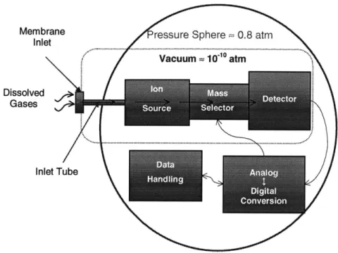
The MIMS instrument is designed to be self-contained, operating within a 17 inch Benthos pressure sphere. The pressure sphere functions to protect instrument components from ambient water, which can reach pressures up to 850 atmospheres. The instrument can be divided into 3 major component groups: the vacuum system, the analyzer, and the electronics system (Figure 3.0-1). The vacuum system consists of a membrane inlet apparatus, inlet tube, vacuum envelope, and ion pump. The inlet apparatus and inlet tube are used to exclude water, while allowing for adequate analyte gas inflow to the analyzer. The ion pump cooperatively maintains a low-pressure environment, permitting analyte gas ion acceleration and detection under free molecular flow conditions within the vacuum envelope. The analyzer component group, which is mostly contained within the vacuum envelope, includes the ion source, cycloidal mass

selector, and Faraday cup detector. Also, positioned outside of the vacuum envelope is a permanent magnet, which provides a homogenous B-field for the cycloid. Together, the analyzer components create analyte gas ions, which are then accelerated along predetermined trajectories toward the Faraday cup detector. Bombardment of the Faraday cup detector by these ions generates an ion current that is then sent to the electrometer. The electrometer senses this ion current and transforms it to an amplified voltage signal. This electrometer output voltage is then converted to a digital signal by a controller/data acquisition (DAQ) board and transmitted to an embedded computer which interprets and

Figure 3.0-1: MIMS conceptual design

Membrane _{ressure Sphere = 0.8 atm}

In let... _{... ...}

Vacuum = 100 atm

Dissolved Gases

Inlet Tube

stores this data. After this data handling is completed, the embedded computer calculates the accelerator potential needed to generate an appropriate trajectory for the next mass value. Using the calculated mass value, the DAQ board generates the correct accelerator potential via a high gain amplifier.

Design and construction of the MIMS package requires analysis and optimization of the three component groups. The remainder of this section seeks to provide the reader with an overview of relevant design issues. Therefore, in an attempt to provide an intuitive format, factors affecting instrument operation are divided into conceptual sub-sections. Each sub-section introduces, in a stepwise fashion, component design & performance issues contributing to overall instrument functioning. They are as follows:

" Vacuum system

Maximum depth capability of inlet apparatus Maintenance of free molecular flow environment " Analyzer

Cycloid performance characteristics Compact, low power design

" Sensitivity

Minimum detectable concentrations of dissolved gases " Response time

Diffusion of gases across unstirred water layer Diffusion of gases across inlet membrane Inlet tube conductance & residence time Electrometer response time

" Computerized control

Automated mass selection & peak height detection Digital accuracy

Sampling frequency " Data handling

Storage & transfer Spectrum separation " Packaging

Layout

Housing & mounting frame

e Calibration

3.1 Vacuum System

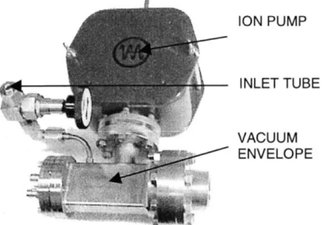
The vacuum system, which houses the cycloid, is comprised of various components including a membrane inlet, inlet tube, vacuum envelope, and ion pump. Space limitations have required that the vacuum system have a compact geometry, yet allow for adequate gas conductance rates. The vacuum envelope is constructed of welded #304 stainless steel and contains the ion source, mass selector, and detector. Roughly the size of the soft drink can (Figure 3.1-1), it was designed to be small enough to fit within the pressure sphere, yet permit satisfactory conductance of excess gases into the ion pump.

Sample gases first diffuse from the water column in through the membrane inlet, then move down the inlet tube into the vacuum envelope. Once gas molecules enter the

vacuum envelope, they are ionized and then accelerated through the mass selector, finally impacting the Faraday cup detector.

Figure 3.1-1: Vacuum system

ION PUMP

INLET TUBE

VACUUM

ENVELOPE

3.2 Inlet apparatus

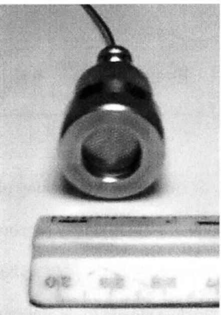
The inlet system, which is to be positioned outside of the pressure sphere, is designed to exclude water, while allowing for adequate analyte inflow by means of a hydrophobic membrane capable of maintaining an internal vacuum of 108 Torr. A physical challenge for marine deployment of the membrane inlet system is to withstand hydrostatic pressures up to 580 atmospheres. The inlet consists of an annular stainless steel cap threaded onto a stainless steel inlet body. Between the inlet body and cap are a stainless steel and a Teflon washer in series, which secure a 1mil thick polymer membrane over a stainless steel micro-etched backing plate (Figure 3.2-1) (see also APPENDIX C: Inlet apparatus Ortho cut away view, pp. 89). Possible failure modes include backing plate collapse caused by excessive hydrostatic pressure, membrane rupture caused by excessive hydrostatic pressure, as well as excessive water vapor influx across an intact membrane due to a thermally or chemically induced increase in membrane permeability. In addition to the problems associated with a catastrophic failure

of the inlet, significant water vapor input can cause a reduction in signal response through the collision of water molecules with analyte ions. A variety of polymers have been investigated for use as a hydrophobic semi permeable membrane (Richardson 1988; Ernst 1994), low-density polyethylene (p = 0.914) having the most desirable strength and permeability qualities.

Figure 3.2-1: Inlet apparatus

Determination of the maximum operational depth limit of the inlet system requires strength calculations (hydrostatic pressure loading) for the stainless steel backing plate and polymer membrane. The membrane can be modeled as an edge held, uniformly loaded circular diaphragm of uniform thickness, without flexural stiffness (Roark and Young 1975). To calculate maximum membrane loading, membrane vertical deflection at the center is first determined (Equation 1),

Tipsi alin]2 _ y[in] y__n

Equation 1: =

K

K4

t]2n

E[Psi] t[in] tdin] t[in]

where t is the membrane's tensile strength (psi.), a is radius (in.), E is modulus of elasticity (psi.), Ki-K4 are proportionality constants, q is maximum load (psi.), t is

membrane thickness (in.), and y is vertical deflection (in.). The deflection term is then used to solve for maximum loading (Equation 2).

IYin]

E[]siln] nK +K 2

j

Equation 2:

qlpsi

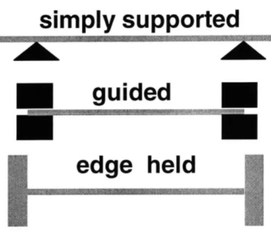
Three general ways of supporting the backing plate are possible: simple, guided, and edge held supports (Figure 3.2-2). A simply supported plate allows for flexing of the plate at its edges as well as movement of the plate with respect to the support as the plate deforms under load; thus, only making use of the unsupported area's rigidity. By contrast, the guided support does not allow for flexing of the plate at its edges, but does allow the plate to move with respect to the support; thereby utilizing the unsupported area's rigidity and the supported area's rigidity leveraged against the support edge. The edge held regime does not allow for flexing of the plate at its edges nor the movement of the plate with respect to the support; thus resulting in a "tensioned" support of the plate. However, a precise edge condition is unlikely, and a truly fixed edge is especially difficult to attain. Even a small horizontal force at the line of contact may appreciably reduce the stress and deflection in a simply supported plate; however, a very slight yielding at fixed edges will

greatly relieve the stresses there while increasing the deflection and center stresses (Roark and Young 1975).

Figure 3.2-2: Types of supports

simply supported

guided

edge held

The empirical equation used to describe yield strength of a circular, uniformly loaded, simple support (Equation 3) is nearly identical to the equation used to describe the yield strength of an edge held plate regime (Equation 4) (Roark and Young 1975).

Equaton 3 q~pil - T psi]X t[in ]2 X

16

Equation 3: qlpsi]=

6

a

(3

Equation 4: q[psi]=

d-

6

(I

In both these equations v is the material's Poisson's ratio (unitless), t is tensile strength (psi.), a is the disk radius (in.), q is the maximum loading (psi.), and t is thickness (in.). The difference between the two equations is only the value of the Poisson's ratio addend. Given #304 annealed stainless steel's characteristic Poisson's ratio of .28, a backing plate

utilizing an edge held support is stronger than a simple support by a factor of approximately 2.5.

The inlet system uses a backing plate support that can be approximated as a quasi-simple support. To avoid over estimation of the plate strength, an equation based on the simple support equation is used which has been augmented with an additional term. This term, V, is included to account for decreased strength caused by the micro-etched holes, and is expressed as the backing plate's surface area to hole void ratio. Using this derivation, a lower limit of the backing plate yield strength can be calculated (Equation

5).

T ps

q[psi]- 6iX t

Iin]2

16

6 X

Once the maximum loading of the membrane and plate have been calculated, a maximum depth rating for each can easily be found. Based on these calculations, the backing plate has a predicted maximum depth rating of approximately 95 meters, while the membrane is predicted to have a maximum depth rating of 118 meters. Although the calculated yield strength of the backing plate is 18% less than the membrane, the support method used for the backing plate is likely to be a hybrid of the simple, guided, and fixed supports. Therefore, the backing plate may actually be stronger than the membrane. Preliminary tests show that the inlet system is capable of withstanding hydrostatic pressure to an equivalent of at least 74 meters depth. Further, destructive testing is needed to ascertain the absolute depth capability of the inlet system.

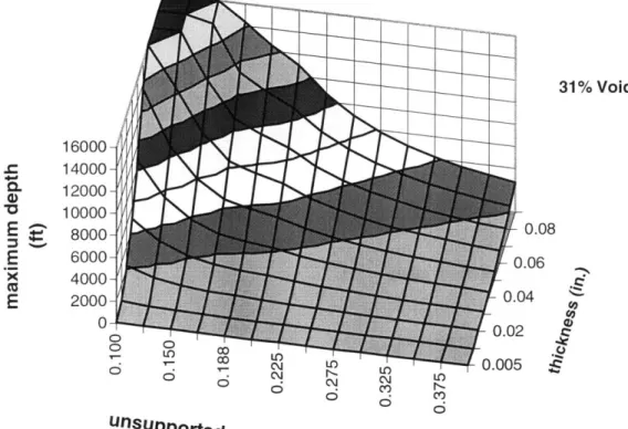
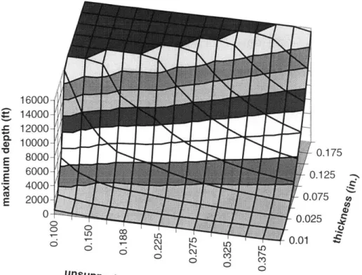
Modifications such as usage of an edge held backing plate, increase backing plate thickness, as well as additional backing plate support using a honeycomb type

reinforcement (Figure 3.2-3), increasing membrane thickness and decreasing the unsupported membrane radius may dramatically increase inlet system depth capability

(Figure 3.2-4) (see also APPENDIX D: Tables of inlet backing plate and membrane depth limits using various design specifications, pp. 101-102).

Figure 3.2-3: Backing plate depth rating

31% Void 16000 -.c 14000 -CL 12000-4) 'a 10000/ E 8000 - 0.08 E 6000-00 40 E 2000 0-04 0 0.02 C~j 4 0.005 0 unsuppOrted aperture N

radius (in.)

16000 E 14000-5 12000-C. @" 10000- 8000-M 6000-E - 4000 E 2000 0")₀ 0 010 co ~- cc 67 6 C\j 1O N ₀ \ r- LO 1 0 C Ij C ~) r-C; C C6 unsupported

aperture radius (in.)

0.175

0.125 >

0.075

0.025 _Q

0.01 $

Figure 3.2-4: Membrane depth rating

7000' .c6000- e5000-1E 4000 5.50E-03 33000 _4.50E-03 E2000 2.50E-03 o ni 1.50E-03 0 6 _5.OOE-04 $ 0 ₀ 21% Void

3.2.1 Vacuum envelope

Aquatic samples of dissolved gases contain water in concentrations of approximately 55 moles per liter, while dissolved gases of interest are nominally of micro-molar to nano-molar concentrations. Because water vapor is the most abundant gas to enter the vacuum system, far in excess of all other gas species combined, the steady state pressure within the vacuum envelope can be estimated based on water vapor influx alone. Assuming water vapor on the outer surface of the membrane is in equilibrium with the ambient water, water vapor pressure on this surface can be determined. Considering that the volume of the vacuum system remains constant, mass in must equal mass out for vacuum envelope internal pressure to be maintained at steady state (i.e. water vapor influx rate equaling vacuum envelope conductance multiplied by internal pressure). To estimate steady state vacuum envelope pressure, the influx rate of water,

Q

@STP/sec), is first calculated, using the permeability coefficient of water across the membrane, P ([cm3@STP-cm]/[cm2-sec-atm]), the membrane surface area, A (cm2_{), and}

the membrane thickness, 1 (cm); where the internal partial pressure of water, p2 (atm), is assumed to be negligible and the external membrane water vapor pressure, pi (atm), is a function of temperature (Equation 6) (Comyn 1985).

(cm3@stp)-cm 2

\m3@sTP [cm sec at

(

[cmp

Equation 6:

[cST

This influx rate,

Q,

7) (see also APPENDIX D: Vacuum envelope steady state pressure determination, pp. 100).

L -atm]

Equation 7: Pss [atm] = ec

F[ L_Fsec

For the purpose of estimating gas conductance, the vacuum system can be modeled as a series of long rectangular and circular tubes which are maintained at pressures that allow for free molecular flow (Duschman 1962) (see APPENDIX D: Conductance determinations for vacuum system components, pp. 99).

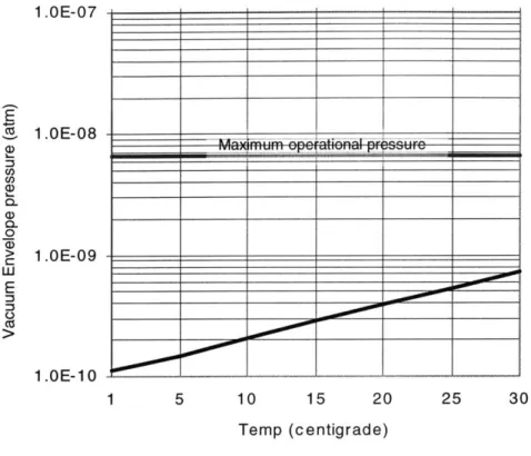
Water vapor pressure is a function of temperature, consequently the steady state vacuum envelope pressure exhibits a temperature dependence. For the specific parameters of the vacuum envelope, a steady state operating pressure of approximately

one order of magnitude less than the operational limit can be expected (Figure 3.2-5). To

maintain a pressure of less than 10~8 Torr, thereby preventing filament burnout and allowing for adequate mean free path length, excess gas molecules within the vacuum system are sequestered by an eight liter per second diode-type ion pump. However, ion

pumps only operate effectively at pressures less than 10-4 Torr. Therefore, initial pump

down must be performed using a mechanical vacuum pump. To further reduce water

vapor associated vacuum envelope pressure and analyzer interference, a KMnO4

Figure 3.2-5: Steady State Vacuum Envelope pressure 1.OE-07 _ 1.OE-08 0. a) > 1 .OE-09 C E Ca) 1.OE-1 0 1 5 10 15 20 Temp (centigrade) 25 30

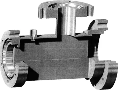
The vacuum envelope is constructed of #304 stainless steel. It consists of a 3 3/8 inch diameter O-ring type flange welded to a 2 x 3 inch (0.049 inch wall thickness) box section tube. The box section is in turn is welded to a 2 % inch conflat flange at its other end. This flange is bolted to a 2 % inch diameter dual BNC feedthrough to allow for connection of the electrometer to the internal Faraday cup. At the center of the box section a linch diameter half nipple (2 3/4 inch diameter conflat flange) which provides an

outlet port to the ion pump. On the box section, between the half nipple and the feedthrough, is the inlet tube (Figure 3.2-6) (see also APPENDIX C: Vacuum envelope Ortho view & Side view, pp. 91-92). The inlet tube fitting is sized to accept an inflow tube attached to a modified heater plate on the cycloid (see also APPENDIX C: Cycloid heater box Ortho view, pp.90).

t ____________________________

Mammum eperatienal

-PON--Figure 3.2-6: Vacuum Envelope cutaway view

The cycloid is held in place within the vacuum envelope via an eight hole bolt through retaining ring that is secured to the 3/8 inch diameter flange. High vacuum is maintained with a 2.112 inch diameter PTFE Teflon O-ring (0.103 inch thickness) positioned between the cycloid base flange and the 3/8 inch diameter vacuum envelope flange. Teflon was chosen over other materials based on its relative low permeability to gasses, ability to withstand high temperatures that occur during bake-out, and low cost compared to single use gold gaskets.

High vacuum testing of this vacuum envelope, using a Varian 200 L/s oil diffusion pump with a CEC model GIC-100 ionization gauge, has confirmed the ability to maintain pressures as low as 3.5 x 10~8 Torr. Additional testing using a Varian 8 L/s ion pump with a Varian VacIon model 921-0012 pump control unit has demonstrated current

draw as low as 21 gamps at 3.8 kV, corresponding to an approximately equivalent pressure.

3.3 Analyzer

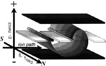
The MIMS employs a modified CEC 21-620 cycloidal type analyzer which uses orthogonally crossed fixed homogenous magnetic and variable homogenous electric fields to impart trochoidal trajectories to sample ions (Figure 3.3-1). Although cycloidal type analyzers are somewhat uncommon, having been largely abandoned by the scientific community three decades ago, this analyzer was chosen over other types of analyzers for several reasons. The cycloidal geometry has the uniquely inherent property of perfect direction and velocity focusing (Bleakney and Hipple 1938), making the analyzer less sensitive to misalignment and vibration. Additionally, because the ion trajectories loop in on themselves a relatively compact flight path, and therefore size, is achievable. The 21-620 cycloidal geometry allows for adequate mass range (2-150 AMU), and a mass resolving power of 100 (Kiser 1965), permitting detection of dissolved biogenic gases, atmospheric gases, light hydrocarbons, and the differentiation of many isotopes.

Figure 3.3-1: Cycloidal ion trajectory

Electric field for the cycloid is produced by a high voltage operational amplifier which supplies a variable potential to accelerator plates within the analyzer. Ions are produced using a heated tungsten filament. Thermionically emitted electrons from the filament are accelerated by a 70volt potential to ionize analyte molecules which enter the ionization chamber. Total instrument power consumption will be kept to a 25 watt maximum by using a high efficiency, frequency modulated, filament emission regulator (see APPENDIX A: Emission regulator circuit board layout, pp. 74) and through the use of a permanent magnet to generate the required 3500 Gauss field across the analyzer. The magnet will be constructed in a U-shaped geometry, with an air gap of 1 inch and pole piece diameters of 3.5 inches. Mass will be reduced to approximately 9 kg by fabricating the magnet of NdFeB, with Permendur 49/49/2 alloy pole pieces and yoke (Figure 3.3-2) (also see APPENDIX C: Mechanical drawings, pp. 92-94).

Relative abundance of gases are determined by ion current collection using a Faraday cup. A Faraday cup detector is the only type of sensor possible for the cycloid. Although Faraday cup detectors are less sensitive than other types of sensors (e.g. electron multipliers), Faraday cups do possess the inherent advantages of low power consumption and long-term signal stability. Used in conjunction with a low noise electrometer, the detector is capable of sensing ion currents as low as 10-14 amps.

3.4 Sensitivity

The inlet system allows for diffusion of analyte gases across the inlet membrane. Given the membrane thickness, surface area, permeability of the membrane to a gas, and the equivalent partial pressure of dissolved gas, a volumetric flux rate of the analyte gas can be estimated. Previous experimentation using a calibrated argon source has indicated that the analyzer requires a minimum gas influx rate of approximately 10-42 grams of argon per second (Hemond), or approximately 2.5 x10-14 _{moles of gas per second, to}

generate a detectable Faraday cup signal. Using this data, minimum MIMS detection limits of individual gas species can be estimated. The minimum mass flux rate of 2.5

x1O-14 moles/sec can be converted into a minimum volumetric flux rate of 5.6 x10-10

cm3/sec at STP. This flux rate, Q (cm3 @STP/sec), can then be used to find the equivalent partial pressure, p, (atm), of the gas encountered on the external surface of the membrane (Equation 8) (Comyn 1985),

p

m

@STP-cm ]A[m2]

Equation 8:

Q

P

where permeability coefficient, P ([cm3_@STP-cm]/[cm2_{-sec-atm]), of a given gas within}

the membrane, the membrane surface area, A (cm2_{), and membrane thickness, 1 (cm), are}

known, and the internal partial pressure of the gas, P2 (atm), is assumed to be negligible. From this partial pressure, an estimate of minimum detectable dissolved gas concentration can be calculated using Henry's law (see also APPENDIX D: Minimum sensitivity determination, pp. 95-98). Although this model does not account for variables such as variability in ionization efficiency or fragmentation, sensitivity estimates based on the inlet system's physical characteristics correspond reasonably with observed detection limits using this inlet system in conjunction with the Hemond backpack mass spectrometer (Allen 1996) (Figure 3.4-1). These sensitivities will permit MIMS measurement of many common dissolved gases (e.g. argon, carbon dioxide, oxygen, and nitrogen) (Seinfeld and Pandis 1998) at ambient concentrations in the ocean, as well as other gases (e.g. helium, hydrogen, methane, and hydrogen sulfide) where they occur at elevated concentrations, such as in waters receiving hydrothermal vent fluids, and in anoxic basins (Welhan and Craig 1983; Morel and Hering 1993; Ishibashi, Wakita et al. 1994) (Figure 3.4-2).

Figure 3.4-1: MIMS minimum sensitivities Argon Benzene Carbon dioxide Carbon monoxide Bhane Helium w rvbthane Ntrogen CD _Oxygen Fantane Ropane ropene TCE

III

rea

LI !'m

''IrIt

A ,

ihiuiii

in~Iuiui'i

Ill-mimi

emeen~em

1 10 100

Concentration (ppb mass fraction)

0.1 1000

IWK 1111110711ffll

E Masured j redicted

Figure 3.4-2: MIMS minimum sensitivities vs. environmental concentrations o3 WAS Sensitivity OAtospheric Equilibrium N Mbrine source

___NU

___

H

-=

3.4.1 Ionization efficiency

Estimation of instrument sample to signal ratio (approximately equivalent to ionization efficiency) is obtained by comparison of measured minimum electrometer signal threshold against measured minimum analyte influx rates. Given the electrometer

input response threshold of 10-4amps, that Faraday cup current is equal to ion current

and electrometer input response threshold equals Faraday cup ion current, approximately 60,000 atoms per second are required to generate a minimum detectable signal. By comparison, the observed achievable minimum detection Argon influx rate of 10-42 grams per second, indicates that a minimum influx rate of 1.5x 1010 atoms per second are needed to generate a detectable Faraday cup signal. Therefore, the sample to signal ratio of the instrument, represented as minimum Faraday cup signal divided by minimum influx rate, is approximately 4.1 x 10-6 (ions detected per molecules sampled).

Further improvements in instrument sensitivity may be made through utilization of inlet membranes with improved permeability characteristics, increasing the permeable surface area of the inlet membrane, as well as improving the ionization efficiency of the instrument. Of these possible modifications, improvement in ionization efficiency is presumably of greatest benefit. Increases in permeable surface area have the disadvantage of allowing proportionate increases in water vapor influx. Although utilization of alternative membrane polymers is likely to increase the sensitivity of the instrument to a given gas or group of gases (e.g. hydrophobic organics) it is unlikely, given current polymer technology, to identify a polymer with superior permeability characteristics for all gases of interest. In contrast, ionization efficiency increase has no directly associated disadvantages and has the potential for order of magnitude improvements, producing concomitant increases in overall instrument sensitivity.

3.5 Response time

Although a steady-state model is used to estimate sensitivity, several factors result in a non-instantaneous instrument response, including electrometer response time, vacuum system conductance, membrane diffusivity, and diffusivity of gases across the unstirred water boundary layer. The contribution of each delay factor to the instrument's overall response time is unequal. Therefore, the following order-of-magnitude analyses serve to identify the limiting factors for instrument speed.

3.5.1 Membrane

The time required for gases to cross the membrane into the vacuum system can be predicted based on the diffusivity of a given gas within the membrane and on membrane thickness. Provided that the diffusion coefficient of the gas through the polymer is independent of concentration and constant, Fick's second law of diffusion (Equation 9)

_C

(2C

Equation 9: - -D I

at X 2)

can be applied as a one dimensional diffusive transport model to estimate the rate of gas permeation across the membrane as a function of time, as the system approaches equilibrium (Allen 1989). If the gas concentration on the external surface is kept constant and gas concentration within the vacuum system is effectively maintained at zero, the total gas flux into the vacuum system per permeable surface area,

Qt,

[ 1

]-

Equation 10:

Q

t

X

6D

As t approaches oo, a linear relation between Q, and t develops, yielding a t-axis intercept, often referred to as time lag, L (sec) (Crank 1975). This time lag can be expressed in terms of membrane thickness, X (cm), and membrane diffusivity, D (cm2_{/sec) (Equation}

11).

X

[c

]2

Equation 11: L[sec]= 6D[cm2

Observation suggests that steady state flow is underestimated by about 4% if a period of approximately three times the time lag is used (Jenkins, Nelson et al. 1970). Applying this time constant of 3L as an estimate of membrane response time, it is evident that membrane thickness strongly affects response time. Given a 1mil membrane thickness, time responses for low molecular weight gases are generally on the order of 10 seconds, with higher molecular weight organics having increased response times (Figure 3.5-1).

Figure 3.5-1: Calculated membrane response time Argon Carbon Dioxide Carbon Monoxide Ethane Helium ai Methane U) Nitrogen Oxygen Propane Propene 0 1 10 100 Time (seconds) 3.5.2 Boundary layer

To the extent that the membrane represents a no-slip boundary condition for water, turbulent transport near the membrane is retarded (Batchelor 1992). Within this

stagnant boundary region, transport of gases normal to the membrane surface is principally through molecular diffusion. Stagnant boundary region thickness may be eroded through increased mixing, but is commonly on the order of 10 to 100 gm for water. A maximum water layer response time for the inlet system can be inferred from the diffusion coefficient of the gas of interest in water. Given that the ratio of two gases' molecular diffusion coefficients in water, D, is approximately equal to the inverse of the ratio of the square roots of their molecular weights, MW, (Equation 12:) (Hemond and

* II

1111111 III

imimim

Eu iiiiiiiiii

imi

iii

ii~~

I

mmmiii

mmiii

mum

mmiii

mum

mmiii

mliii

Fechner 1994), and using a diffusivity constant of 1.7 x10-5 cm2/sec for carbon dioxide in

water, the diffusivity of other molecules in water can be approximated (Figure 3.5-2).

Figure 3.5-2: Mass dependence for molecular diffusion in water

8.E-05 5.E-05 -E : 3.E05 -1. E-06 2 22 42 62 82 102 122 142

Molecular weight (AMU)

DA [MWB [AMU

Equation 12: D |

DB 1cm Vecj I MWA [AMU

Assuming that the largest analyte gas of interest will have a mass of 150 AMU (i.e. the MIMS mass range limit), a minimum diffusivity can be calculated and applied to the time-to-steady-state lag model. Using a worst case stagnant boundary layer thickness of 100pm, the maximum water time lag for any molecule within the analyzer's mass range is no more than approximately 5 seconds (Figure 3.5-3), and could be decreased by local stirring if necessary.

Figure 3.5-3: Water boundary layer time lag 6 -5 -- - - -25um C~ 50um 0a 0 ~e-75um ! 4 100 um0 0--3.5. Inlt li e e 0 2-t[A] 44. 0 Moeua eih AU 2t 22dctne 42 62mc 82q102i1221142

tsc

Equtin.

₃

_.

Gas tpravl fromste mftembranueneoe anlris anxiadtional0- sorce oft tme

moel.hre trae tiesn to sec)risimly he voum ofal theine tube, Vn (cthiieb

assuming molecular flow conditions (Duschman 1962). In a molecular flow regime, conductance is a function of container geometry, temperature, pressure, and molecular mass; however, it is not dependent on pressure. Using Clausing's approximate solution for conductance (Clausing 1932), a long narrow tube's conductance, F (cm3/sec), is determined by: tube cross section, A (cm2); temperature, T (Kelvin); molecular mass, M (AMU); and a dimensionless parameter, K, which is determined by the tube's length to cross sectional area ratio (Equation 14) (see also APPENDIX D: Conductance determinations for vacuum system components, pp. 99).

Equation 14: F[m _{F ,c}

]=

Calculations using this model indicate that tube length has the greatest influence on residence time. Based on this analysis, analyte gases of interest have residence times of roughly 1.5 seconds when inlet tube length is 50 cm (Figure 3.5-4).

Figure 3.5-4: Inlet tube residence time

Argon Carbon dioxide Carbon monoxide Ethane o Helium 15 Methane CD Nitrogen Oxygen Propane Propene Water 0 0.5 1 1.5

Residence time (sec)

2 2.5

-I-I-I--

-

--

-

~.

-

-

-

m

-

-

~.

-

-

-

--

-

-

-

--

-I-I-3.5.4 Electrometer

The response time of the electrometer can be described by its RC time constant. The electrometer is based on a Teledyne 1702 op-amp connected as a current-to-voltage converter, followed by a unity gain inverting buffer (Figure 3.5-5). The 1702 has an extremely low bias current achieved with a parametric input stage. A 10"Q feedback resistor is used in parallel with a 2pF capacitor, giving a response time of approximately one half second.

Figure 3.5-5: Electrometer schematic

11 10 Q /\fN 100K Q Ion Current Input ~~~ - 100K Q .01 F 308 Output Voltage +15 -15

3.5.5 Overall response time

Drawing from the preceding analyses, it is expected that MIMS/AUV response time will be primarily governed by membrane diffusivity if relatively few gas species are being measured, and will be of the order of 10-20 seconds. If successive scans of the entire spectral range are required, electrometer response time may become the limiting factor. For example, if 200 mass peaks (including molecular ions and fragments) are measured per scan, and measurement of each peak requires 0.5 second, the time needed

to complete the scan would be 100 seconds. Further electrometer analysis and re-design may allow for a decreased time constant. Modifications such as use of a smaller input resistor in the first stage would decrease response time and have the added benefit of lowering the resistor's Johnson noise contribution, but would require more detailed analysis of all system noise sources. Development of data interpretation algorithms that predict final electrometer output in advance of the system reaching a steady state value may also help. In a future design, using an electron multiplier instead of a Faraday cup, detector response time could be decreased to milliseconds, under which conditions it would not be a factor.

3.6 Computerized Control

Autonomous operation requires that the MIMS instrument be able to perform all necessary functions via a pre-programmed embedded computer system. Minimum functionality includes powering instrument on & off at predetermined intervals, mass step calibration, accelerator potential control, emission regulator control, data collection & handling, and systems diagnostics. To fulfill these operation needs as well as power and space limitations, the MIMS will use an embedded PC- 104 computer coupled with mass selector controller and data acquisition system. The MIMS computer will use a serial port connection to communicate with the AUV control computers.

The controller/data acquisition system, or DAQ board, was designed to function as a compact (12cm x 9 cm), low power (1.5 watt), 16-bit resolution controller and sensor (Figure 3.6-1). It is compatible with computers using 8X86 through Pentium® microprocessors, and interfaces via a printer port employing a PS-2/bi-directional protocol (IEEE1284). The IEEE 1284 standard allows for a maximum data width of

8-bits. Consequently, the DAQ board makes use of a multiplexor array, which allows for a "two pass" 16-bit transfer of both controller and sensor data. The DAQ board relies on an Analog Devices 569 digital-to-analog converter to "write" commands to the mass selector and an Analog Devices 7884 analog-to-digital converter to "read" electrometer voltage. Both the 7884 and the 569 possess sample-and-hold capabilities, permitting simultaneous operation of the DAQ's input and output.

Figure 3.6-1: DAQ board

I I k*

3.6.1 Power

During the development and testing of the DAQ board, an Hewlett Packard 6236B controlled voltage source was used to supply the +5V and -5V required and an Heath 2718 to supply +12V and -12V. The DAQ board consumes approximately 1.5

watts of power, requiring a +5V supply sourcing 20 mA, a -5V supply sinking 20 mA, a +12V supply sourcing 40 mA, a -12V supply sinking 40 mA, and GND.

3.6.2 Board fabrication & layout

The DAQ board was fabricated from a dual sided copper photo-etched board. Photo-resist etching mask negatives were drawn using TurboCAD version 2.0 software. The footprint of the DAQ board measures 4.8 x 3.5 inches and is designed to be compatible with PC-104 form factor. The DAQ board is in its third generation of design and is denoted as PARADAQ version 3.1 on the board surface (see Appendix A: PARADAQ and emission regulator circuitry). Previous design generations employed a prototype Analog Devices AD7882 analog-to-digital converter which has since been abandoned by Analog Devices, because of bugs within the converter. The board is designed to allow for sockets to be soldered into place, permitting replacement of individual integrated circuits. All socket pads are designed for DIP integrated circuits. Future versions of the DAQ board can be made smaller by replacing the AD7884 with an

AD7885, which eliminates the need for two of the six multiplexors, and by using

surface-mount integrated circuits.

3.6.3 Software

DAQ BOARD software was written using the Q-Basic language. Q-Basic was chosen because code for the backpack-portable mass spectrometer, which uses an RS232 serial port, was written in Quick Basic 4.0 (Microsoft's predecessor to Q-Basic). The code for the backpack mass spec was modified slightly to accommodate the new parallel port interface. All software written for the parallel port interface requires a computer operating on a MS-DOS platform and possessing a Bi-directional (PS2) parallel port

operating within the HEX address range of &H378-&H37A and using a BYTE mode handshaking protocol (Figure 3.6-2). The DAQ software is not written to support SPP (also known as nibble mode), EPP, ECP, nor FIFO mode handshaking protocols.

Figure 3.6-2: DAQ board timing diagram

CONVST

OS

HBE LBE & LDAC

DATA

HI OUT LOW Out HI IN LOW IN

STAT 7

CTRL 5

CTRL 2 CTRL 1

CTRL 0

All Q-Basic programs written for the DAQ board use direct memory addressing, or DMA, to read and write information to and from a parallel port residing in the computer's LPT1 range. This LPT1 address corresponds to a hexadecimal address of 378h. From this address, the three parallel port registers can be accessed: the data register at 378h, the status register at 379h, and the control register at 37Ah. Operation of the DAQ board is accomplished via a standard execution code for IEEE-1284 standard bi-directional parallel port equipped computers (see APPENDIX B: Standard PARADAQ execution code pp. 81). A modified execution code has been developed for computers such as the Toshiba T1000 notebook computer, which uses a variation on the IEEE-1284

standard (control bit 7 replacing the functioning of control bit 5)2 (see APPENDIX B: Toshiba T1000 PARADAQ execution code, pp. 85). Analog-to-digital converter command values for the Toshiba T1000 should have a value of 96 added (adding bit 7, and subtracting bit 5).

The output portion of the code first writes the output values to the AD569 in a "two pass" method, then the input commands switch the control register lines to read the data register AD7884 input values, in a "two pass" method as well (Figure 3.6-3).

Figure 3.6-3: DAQ board controller subroutine

MSB = INT(BITCNT / 256)

LSB = INT(BITCNT - MSB * 256)

REM OUTPUT TO DA CONVERTER FIRST HIGH, THEN LOW OUT &H37A, 4 OUT &H378, MSB OUT &H37A, 0 OUT &H37A, 4 OUT &H37A, 6 OUT &H378, LSB OUT &H37A, 2 OUT &H37A, 6 OUT &H37A, 4

REM INPUT READ FROM AD CONVERTER OUT &H37A, 165 OUT &H37A, 164 OUT &H37A, 165 hibyte = INP(&H378) OUT &H37A, 167 lobyte = INP(&H378)

inbits = (hibyte * 256) + (lobyte)

2 The IEEE 1284 standard specifies that control register lines 0,1, and 3 use inverted