HAL Id: hal-03023850
https://hal-amu.archives-ouvertes.fr/hal-03023850
Submitted on 25 Nov 2020
HAL is a multi-disciplinary open access
archive for the deposit and dissemination of
sci-entific research documents, whether they are
pub-lished or not. The documents may come from
teaching and research institutions in France or
abroad, or from public or private research centers.
L’archive ouverte pluridisciplinaire HAL, est
destinée au dépôt et à la diffusion de documents
scientifiques de niveau recherche, publiés ou non,
émanant des établissements d’enseignement et de
recherche français ou étrangers, des laboratoires
publics ou privés.
Imaging multiple cortical areas with high
spatio-temporal resolution using innovative wide-field
imaging system
Manon Bourbousson, Isabelle Racicot, Eduard Muslimov, Thibault Behaghel,
Kévin Blaize, Audrey Bourdet, Sandrine Chemla, Emmanuel Hugot, Wilfried
Jahn, Sébastien Roux, et al.
To cite this version:
Manon Bourbousson, Isabelle Racicot, Eduard Muslimov, Thibault Behaghel, Kévin Blaize, et al..
Imaging multiple cortical areas with high spatio-temporal resolution using innovative wide-field
imag-ing system. SPIE Photonics Europe 2020, Mar 2020, Online, France. pp.1136002. �hal-03023850�
Imaging multiple cortical areas with high spatio-temporal
resolution using innovative wide-field imaging system
Manon Bourbousson
a, Isabelle Racicot
a,b, Eduard Muslimov
a, Thibault Behaghel
c, K´
evin
Blaize
b, Audrey Bourdet
b, Sandrine Chemla
b, Emmanuel Hugot
a,c, Wilfried Jahn
c, S´
ebastien
Roux
b, Ivo Vanzetta
b, Pascal Weber
b, Jean-Fran¸cois Sauvage
a,d, Fr´
ed´
eric Chavane
b,*, and
Marc Ferrari
a,*a
Laboratoire d’Astrophysique de Marseille: Aix Marseille Univ, CNRS, CNES, LAM,
Marseille, France
b
Institut de Neurosciences de la Timone: Aix Marseille Univ, CNRS, INT, Marseille, France
cStart-up CURVE-One, Marseille, France
d
ONERA, D´
epartement d’Optique Th´
eorique et Appliqu´
ee (DOTA), Chatillon, France
*Co-supervisors
ABSTRACT
Recording brain activity at the mesoscopic scale has a strong potential to unveil many new fundamental neuronal operations. Optical imaging offers a unique opportunity to measure brain activity over a large area with high spatio-temporal resolutions (20 µm x 1 ms). However, two major limitations of this imaging technique partially explain the lack of development in this field. The cortex being non-planar, the field’s depth limits the region in focus to a small region close to the center of the field of view. This is particularly significant for the highly curved lissencephalic small cortex of non-human primates that are becoming popular in neuroscience experiments. The ideal technique would be a method that compensates for such curvature; it would enable imaging the whole visual system at once, from the primary to the fifth visual cortices, in small non-human primates. Additionally, the signal-to-noise ratio is strongly degraded by the dynamic evolution of the brain curvature due to physiological rhythms (heartbeat, breathing, etc.). This strongly limits the ability to work at a single-trial level and to unravel the real dynamics of neuronal processing, such as spatio-temporal waves. Here in this project, we present an interdisciplinary approach for imaging of the non-human primate cortex, using technologies from astronomical instrumentation to overcome current technological limits. This will be of interest to a wide neuroscientific audience but also will impact the clinical community interested in mapping the nervous activity at the mesoscopic scale. Our current preliminary development involves redesigning the illumination source and the optical design. Keywords: Neuroscience, optical imaging, mesoscopic scale, cortex, non-human primate, visual system, curved sensors, LEDs
1. INTRODUCTION
Optical imaging techniques such as intrinsic imaging and voltage-sensitive dye (VSD) imaging are used to record neuronal activity in non-human primates to understand the role of this dynamical activity. They have proven to offer the opportunity to measure the activity over a large field of view with high spatio-temporal resolutions.1,2
Both of these imaging techniques give access to a network of neurons, from the sub-column to a whole area, thus covering the mesoscopic scale.3 However, the optical instrumentation used while performing the measurements
is not fully optimised, limiting further results in fundamental neuroscience research. One of the instrumental limitations very commonly encountered can be illustrated by Muller et al. study.4,5 In the study, two models
of travelling waves mechanism followed by the activity response are exposed. They explain the importance of
Contact author information:
Manon Bourbousson: E-mail: [email protected] Isabelle Racicot: E-mail: [email protected]
unraveling the role of these waves in neural systems at the single-trial level, but they emphasize the lack of larger-scale imaging techniques. Indeed, the propagating waves detected, subject to high spatial-to-noise impacting the ability to work at single-trial, were recorded only from a reduced portion of the cortex region available in the recording chamber. We observe that there is around 70 - 90 % loss of signal information compared to the signal that could be recovered from the entire accessible cortex (chamber diameter 18 mm).
Clearly, to tackle these limitations, more widely described later in this section, efforts in system design are required. In this project, we mainly refer to the uneven illumination of the cortical region of interest and the low image quality as the major limitations. To prepare a typical experimental run in intrinsic imaging, the experimenter is manually adjusting the illumination on the animal’s brain surface using two adjustable lightguides which introduces an element of unreliability and uneven illumination. This gives rise to variability between the measurements of the area from which the signal is recorded, and also to the difficulty to extract the neuronal activity signal in the region less illuminated.
On top of that, the use of commercially available detectors in the current cortical imaging experiments is not optimal. They have planar geometry while the cortex surface imaged is curved. This, combined with the optical design of the instrument which is optimized to create an image of a flat object on a planar image sensor, induces vignetting and image blurring in the field of view (FoV). In other terms, the image formed on the camera sensor is of similar curvature than the cortex itself creating aberrations that could be avoided by an appropriate optical system. In the following paragraphs, we will present the development of a new design based on a curved sensor.
2. ILLUMINATION SETUP
The optical setup considered as a starting point for this project has been used for cortical imaging experiments for over decades as described in 1999.6 It consists in two camera lenses (both SMC Pentax 50 mm, F 1.2) organised in
tandem, oriented front-to-front and connected to a camera (Complementary Metal Oxide Semiconductor (CMOS) sensor, Photonfocus, MV1-D1312-160-CL). This system essentially behaves as a microscope with a magnification of 1; it has a high numerical aperture with a shallow depth of field when used at the maximal numerical aperture (F-number equal to 1.2). This system is placed above the macaque cortex to cover the entire area of the cortex (V1 visual area) visible in the cranial optical chamber. For intrinsic imaging and voltage-sensitive dye imaging, the illumination source used is a halogen light source (150 W maximum) oriented towards the sample via two lightguides (Schott). Appropriate filters are placed in the illumination path to select the wavelength of interest which varies with the type of imaging used (typically used wavelengths 570 nm, 605 nm, and 630 nm).
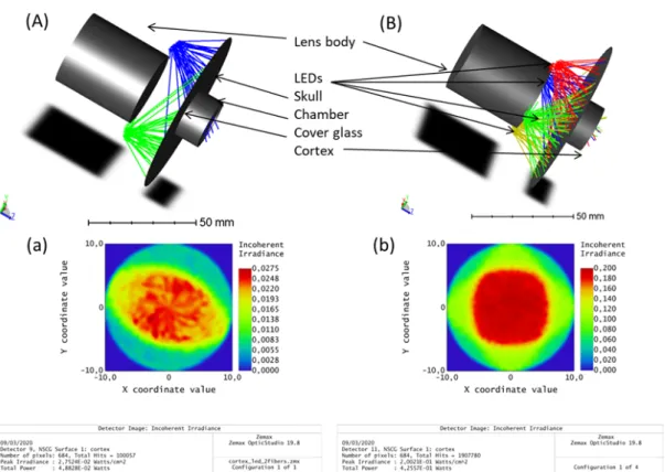
This illumination system is not ideal to create a uniform illumination over the entire cortical area in the imaging chamber. The light source is manually directed towards the animal cortex to maximize the uniformity of the illumination as measured by the recording camera. The geometry of the two lightguides, however, cannot theoretically create a uniform illumination over the whole area covered by the chamber as illustrated in Fig.1(a). On top of that, this light source emits a lot of heat.
For all these reasons, the current illumination system is not optimal: we, therefore, designed a new illumina-tion system based on several symmetrically posiillumina-tioned light-emitting diodes (LED). The advantages of LEDs are their fast response rates, fast stabilization after their warming up period, additionally, they consume less energy, produce less heat and have higher output stability than halogen source. LEDs have been used in neuroscience with encouraging results.7,8 The design of our new illumination system consists of 4 LEDs (Osram LZ4-20MA00) placed around the camera lens body and oriented at a specific angle that maximizes the overlapping region of the light emitters and its uniformity. The LEDs are powered by a very stable DC power source which yields an appropriately temporally stable illumination.
Both systems: the currently used one and the newly developed and their corresponding simulated illumination are compared. Fig. 1 displays the 3D layout of the two systems with the second lens body represented with the two different illumination designs as well as the Zemax simulated detector view plot corresponding to the cortex’s surface.
In this situation, we considered a chamber of 20 mm inside diameter, the largest recording chamber used. As illustrated by the Zemax simulations, the original illumination design represented in Fig.1(A) present a distorted region of maximized illumination as seen on the detector view plot (Fig.1(a)). We notice a peak of irradiance
Figure 1. Illustration of the illumination system (A) in the original setup and (B) in the optimized light-emitting diode (LED) design. We present the layout of both configurations (A) and (B) as well as the detector view (smoothing 10, false color) corresponding to the cortex surface in (a) and (b) respectively.
shaped like an ellipse and various spots of light. Hence, in this configuration, only a minimized region is properly illuminated which corresponds to a small region of the region of interest where many regions of the chamber are underexposed. The region of illumination is covering 85 mm2 of the surface representing 27 % of the total area available (314 mm2). On the other hand, for the optimized LED design displayed in Figure 1(B), the area is uniformly illuminated over a larger region (Fig.1(b)). In comparison, the area of illumination is not only made homogeneous but also enlarged by a factor 1.5 with the system we developed.
We have confirmed that our LED-based illumination design substantially improves the uniformity of the illumination and the region covered. Once the illumination setup was redesigned, we then focused on the redefinition of the optical setup.
3. CURVED SENSOR
An innovative solution, based on advances in manufacturing technologies consists of curving the sensor. This is performed by the start-up CURVE-One, a specialist in curving any sensor to a required shape. For our project, the sensor curvature will be used to compensate for the curvature of the observed object: the macaque cortex. To quantify the desired curvature of the image sensor, the first step consisted in the calculation of the radius of curvature of various macaque cortices. To the best of our knowledge, similar calculations have not been reported in the literature. We have had access to a public database of Magnetic Resonance Imaging (MRI) data (from the Cerimed), from which we extracted via an open-source software (Brain VISA Anatomist) the data points corresponding to the surface of the brain included in the recording chamber. From the cloud of points extracted, we applied a spherical fit in Python. We calculated the cortex radii of curvature of 8 macaques; the results are presented in Fig.2. For the calculations, we have included both hemispheres of each macaque, leading to 16 data points in order to get an idea of the spread of the curvature distribution and therefore determine whether or not
our design can be appropriate for many individuals or if we have to specialize the design with a specific macaque in mind. The standard deviations were calculated as the squared root of the diagonals of the covariance matrix.
Figure 2. Data plot of the average radius of curvatures of macaque from our database. For each animal (Maga, Jaffar, Elouk, Cleo, Cesar, Apache, Ziggy and Hip) the left and right data points represent respectively the left and right hemispheres.
We have noticed that the surface of the monkey, reported as Cleo, was particularly irregular for the right hemisphere so it will be considered as an outlier from now on. We obtain for 6 macaques of similar morphology an average of 30 mm ± 8 mm for the cortex radii of curvature (Fig.2(A)). The source of the large deviations around the average seems to be mainly due to local irregular features present at the surface of the cortex. While we found an average value of the curvature, what is more relevant for us is to repeat the calculations on the data from the two animals: Ziggy and Hip we will be working with. As shown in Fig.2(B), the values calculated from their cortex surface are included in the average range of the radii curvatures calculated previously. In conclusion, for the rest of the study, we have set the target object curvature to be equal to 29 mm corresponding to a value included in the average value obtained for theses two animals (28 ± 1 mm).
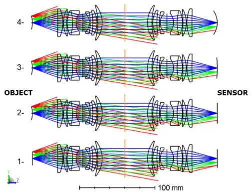
Now that the object curvature is determined, the characterisation of the optical system should be performed. We carried various tests on our laboratory test bench; indeed, we replicated the original setup with as the object of interest: a 3D printed artificial brain (printed from white resin). We used a modular camera that allows us to change camera sensors. Our sensor of choice the AMS CMV12000 was used in two configurations: as a flat sensor and as a concave sensor with a radius of curvature of 200 mm. The sensor was curved and characterised to be functional with good performances by the start-up CURVE. Here, we present the results of the simulations of the different optical designs. We defined a set of configurations in Zemax software (OpticStudio) corresponding to the original setup and variations of the optimised designs (with a combination of flat and curved sensor and flat and curved object). The variable parameters between the configurations are the object shape and the camera sensor radius of curvature. The second configuration represents the original setup, with the spherical brain imaged on a flat sensor. The first configuration assumes that the brain is flat while the fourth configuration assumes the sensor is curved nearly to the same radius of curvature than the brain (35 mm). And finally, the third configuration considers a sensor of 200 mm of radius of curvature representing the theoretical manufacturing limits to the sensor curvature back then. For the simulations, each Pentax objective is represented by the Double Gauss lens design. Its 7-lens design is composed of a combination of optical glasses with different Abbe numbers and refractive indexes. The lenses are placed front-to-front with maximum aperture (corresponding to a F-number of 1.2). An illustration of the configuration’s layout is displayed in Fig.3.
From these, we performed the optical performance quantification and plotted the field curvature, vignetting and root mean square (RMS) spot size vs image field of all the configurations. At first, we generated the
Figure 3. Representation of the four configurations with configuration 1- flat object, flat optical system ; configuration 2-spherical object (29 mm), flat sensor ; configuration 3- 2-spherical object (29 mm), curved sensor (200 mm) and configuration 4- spherical object (29 mm), curved sensor (35 mm).
vignetting plots of our optical systems as shown in Fig.4.
From the vignetting plot, we notice that even for the two most ideal configurations, the system has significant vignetting from the middle to the outer parts of the field; we observe a relative illumination of only 20 % at the edge of the field (9 mm). The losses due to vignetting in the system are considerable. As a first modification, we would propose to bring the front end of the objectives closer to each other, closer than 6 cm set initially. An improvement of the relative illumination of 25 % at the edge of the field would occur by narrowing the distance between the objectives by 1 cm.
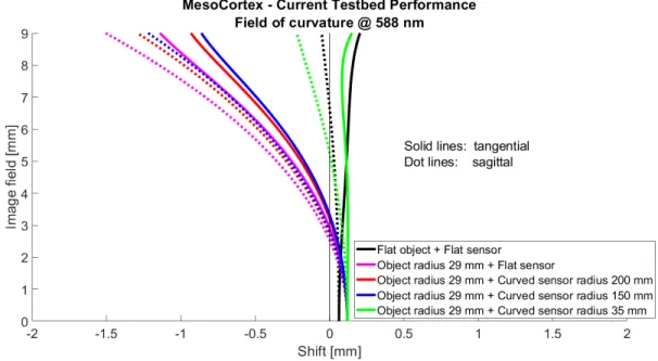
We also plotted the field of curvature curves. In the original configuration, to fit the planar detector, we expect to maximize the flattening of the focal surface. However, as observed in Fig.5, the curve representing the original design (in pink) shows consequent field curvature represented as the shift in mm. It reaches for tangential and sagittal respectively 1.1 mm and 1.5 mm at the edge of the field. These shift values are hardly lowered when using a curved sensor with 200 mm and 150 mm radius of curvature indicating the irrelevance of the use of a curved sensor in this original optical setup. Then, when the sensor is curved to match the curvature of the object, the field curvature aberration is suppressed over the entire image field. In the ideal case of flat configuration, the field curvature is also minimal. From those configurations, we would expect better image performance though they are not realistically achievable situations.
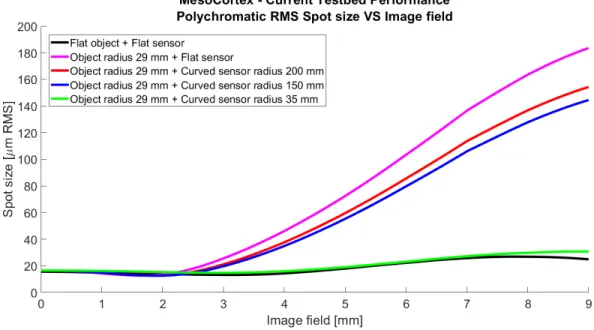
Lastly, in Fig. 6, we represented the root mean square (RMS) spot size as a function of the image field. For the irrealistic configurations, over the entire image field, the zero slope of the curve indicates the absence of geometrical aberrations. The RMS spot radius stays below 25 microns everywhere across the field. In the currently used design, as of 3 mm away from the center of the field, the RMS spot radii increase rapidly reaching the value of 180 µm at the edge of the field. Finally, the improvement in geometrical performance is very small when going from the original design (in pink) to both curved sensor setups (in red and blue). The degradation of the spot radius across the image field suggests that the performance of the system is degraded.
In conclusion, the imaging quality of the design used in neuroscience experiments has been fully characterised. From the simulations of the field curvature aberrations and the image vignetting, we can confirm that the system
Figure 4. Overall vignetting calculated by Zemax corresponding to configuration 1 (in black) and configuration 4 (in green).
Figure 5. Field of curvature plot calculated by Zemax for all the configurations
in use can be optimised for imaging macaque brains. Also, the simulation enhances the fact that swapping the flat sensor with a curved one, in the manufacturing technologies boundaries, does not compensate for the brain curvature. We conclude that the sensor itself as a single optical element is not sufficient to eliminate all the aberrations, so a full redefinition of the system is necessary. This is what we will present in the next section.
4. FUTURE OPTICAL DESIGN
The custom optical design for the imaging system should provide higher resolution and higher image illumination over the entire field of view. The current baseline implies the following system composition (see Fig.7): 1 –
Figure 6. Polychromatic root mean square (RMS) spot size vs image field calculated by Zemax for all the configurations.
curved object, represented by a spherical surface, 2 – chamber with immersive liquid, 3 – double Gauss type custom projection lens, 4 – aspherical corrector lens and 5 – curved CMOS detector.
Figure 7. General view of the customized optical system design for cortical imaging.
The linear field of view limited by the chamber size is 18 mm. The image size should correspond to the sensitive area of a commercial CMOS sensor. For AMS CMV 12000 it equals 22.5 x 16.9 mm, so the linear magnification is -0.94x. The working spectral band is 595 - 670 nm, which allows to cover both the intrinsic and fluorescence imaging modes. Since the object curvature is as steep as 29 mm it is hard to compensate the field curvature by a single element. So this function is split between the curved sensor, which has a radius of curvature limited to 150 mm due to technological boundaries, and an aspherical corrector lens, which also compensates other aberrations across the FoV. We assume that the sensor cover glass will be removed during the curving process, so the corrector can be placed close to its surface.
The custom optical design should account for a few trade-offs. First, it would be highly desirable to work with a low F/# to collect more light and increase the image illumination, which means a higher sensitivity and temporal resolution. On another hand, lower F/# corresponds to a shorter depth of focus, which can become critical when working with an object of irregular shape. Finally, achieving a high resolution becomes a problem at low F/# values, so the lens design can become more complex and difficult in production and operation. To estimate the influence of the mentioned factors we optimized the lens for 3 F/# values for comparison. For the depth of focus computation, we assumed the resolution element size equal to 11µm, which corresponds to pixel binning. We
used module transfer function (MTF) value at 33 l/mm frequency to assess the image quality. The results are shown in Tab.1.
Table 1. Comparison of the projection lens parameters at different F/# values.
F/# 2.5 2.0 1.5 Depth of focus, µm 55 44 33 No. of lenses 7 7 8 No. of aspheres 1 1 2 Min MTF @33 l/mm 0.29 0.28 0.12 Max MTF @33 l/mm 0.69 0.52 0.40
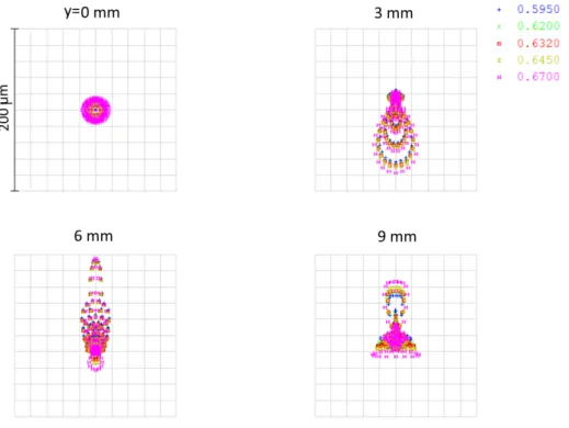
The F/2 configuration represents a compromise decision since the further decrease of the aperture brings only a limited gain in performance and its increase requires complications of the optical design. The focal length, in this case, is 45.7 mm and the total system length is 172.2 mm. The spot diagrams for this configuration are shown in Fig.8. The RMS radius varies from 9.6 to 27.4 microns, the maximum radii are 15.7 - 95.4 microns. One may note that the image quality is mainly limited by astigmatism.
Figure 8. Spot diagrams of the custom projection lens in F/2 configuration for five wavelengths (595 nm, 620 nm, 632 nm, 645 nm, and 670 nm) chosen in the working spectral band.
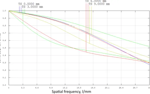
The MTF plots are shown in Fig.9.; they demonstrate that the resolution is quite uniform across the FoV and that it will be possible to resolve the object features down to 30 microns in size even at the field edges.
The relative illumination shown in Fig. 10 varies by ∼28 % from the field center to its edge. This change occurs mainly due to the incidence angle variance and seems to be unavoidable with such a steep object surface. However, this effect is moderated in comparison with a flat sensor-based configuration.
The image distortion was limited during the optimization. The residual pincushion type distortion is 4.7% (see Fig.11).
Figure 9. Module transfer function of the custom projection lens. For all the field positions (0.0 mm in blue, 3.0 mm in green, 6.0 mm in red and 9.0 mm in olive) are represented the tangential (T) and sagittal (S) responses separately.
Figure 10. Relative illumination distribution across the field of view.
Besides, the edge spread function plots are provided (Fig. 12). This measure of image quality is relatively easy to use for a curved irregular object in practice. The width of the edge responses is a quantification of the sharpness loss through the imaging system. As observed in Fig.12, the edge intensity profiles for both directions of the semi-infinite plane and at the center and the edge of the field are almost perfect step functions. The excellent edge response indicates no significant degradation in image quality through our optical system.
Finally, we present the lens characteristics. The aspherical corrector represents a meniscus with asphere on the first convex surface. The asphere is described by a 1st type Q polynomial of 5th order. Its clear aperture is 21 mm and the vertex radius is 13.38 mm. Fig.13 shows the residual asphericity after the best fit sphere subtraction. The breadth-first search (BFS) radius is 15.38 mm, the peak-to-valley (P-V) deviation is 218 µm
Figure 11. Grid distortion diagram of the projection lens in F/2 configuration.
Figure 12. Geometrical edge spread function diagrams for the custom projection lens.
and the RMS deviation is 78 µm.
Figure 13. Departure from the breadth-first search (BFS) in microns for the aspherical corrector surface.
The future step of the MESO-CORTEX program will consist of adding “adaptive/active optics” capabilities in the imaging system, in order to compensate for the dynamic evolution of the brain curvature due to physiological rhythms (heartbeat, breathing, etc.) translating in curvature changes. To address this point, a deformable detector, able to follow the variation of the brain curvature as seen through the optical system, is currently
under study between the CURVE-One company and LAM, based on previous development of variable curvature optics for astronomy. This part will also require the development of a curvature measurement method to control the curvature of the deformable detector. With the residual curvature uncorrected by the optical system evolving with time, a direct measurement in the image is necessary. Two possibilities exist, both having already been implemented in astronomy, even for more complex aberrations measurements than simply the curvature. The first one directly uses the scientific image and a dedicated algorithm to estimate the curvature. It does not require additional optics but translates complexity into real-time analysis and computing power. The second one takes a light projection on the brain, dedicated to the curvature measurement (a different wavelength unused by the science imager), with additional optics but allowing an easier measurement and an extended photometric use (the source module flux can be adjusted easily to adapt to the exposure time). Compensating for dynamic perturbations from physiological rhythms should allow gaining both in terms of corrected field and signal-to-noise ratio, enhancing images at the mesoscopic scale. A trade-off on the measurement method, between system simplicity and measurement performance, will be performed using an already existing physiological data set and, as soon as possible, using data taken with the new imaging system in its static version.
In conclusion, we have adapted tools developed originally for astronomy such as field curvature corrector lenses and curved sensor to develop a new optimised design. We have demonstrated the enormous improvement in the image quality brought by this final design. Blurred regions, uneven illumination and vignetting seen in all the previous configurations are removed.
The use of this optimised design, which provides high resolution and high image illumination, will help to obtain neuronal recordings with improved quality over a large field of view. It tackles the current instrumental limitations and will play an important role in the next fundamental research activities in neuroscience. We hope that the implementation of this design in optical imaging experiments will participate in helping to understand the role of the dynamical activity in the processing of information.
ACKNOWLEDGMENTS
The authors would like to thank Joel Baurberg and Xavier Degiovanni for their technical assistance. We also thank Kep-Kee Loh, Olivier Coulon and David Meunier from INT for their invaluable help processing the brain MRI scan data. We would also like to acknowledge H2020 ATTRACT and CNRS 80 Prime for financial support.
REFERENCES
[1] S. Chemla and F. Chavane, “Voltage-sensitive dye imaging: technique review and models,” Journal of Physiology-Paris 104(1-2), pp. 40–50, 2010.
[2] A. Grinvald and R. Hildesheim, “Vsdi: a new era in functional imaging of cortical dynamics,” Nature Reviews Neuroscience 5(11), pp. 874–885, 2004.
[3] S. Chemla, L. Muller, A. Reynaud, S. Takerkart, A. Destexhe, and F. Chavane, “Improving voltage-sensitive dye imaging: with a little help from computational approaches,” Neurophotonics 4(3), p. 031215, 2017. [4] L. Muller, F. Chavane, J. Reynolds, and T. J. Sejnowski, “Cortical travelling waves: mechanisms and
com-putational principles,” Nature Reviews Neuroscience 19(5), p. 255, 2018.
[5] L. Muller, A. Reynaud, F. Chavane, and A. Destexhe, “The stimulus-evoked population response in visual cortex of awake monkey is a propagating wave,” Nature communications 5(1), pp. 1–14, 2014.
[6] A. Grinvald, D. Shoham, A. Shmuel, D. Glaser, I. Vanzetta, E. Shtoyerman, H. Slovin, C. Wijnbergen, R. Hildesheim, and A. Arieli, “In-vivo optical imaging of cortical architecture and dynamics,” in Modern techniques in neuroscience research, pp. 893–969, Springer, 1999.
[7] D. A. Wagenaar, “An optically stabilized fast-switching light emitting diode as a light source for functional neuroimaging,” PLoS One 7(1), 2012.
[8] B. Salzberg, P. Kosterin, M. Muschol, A. Obaid, S. Rumyantsev, Y. Bilenko, and M. Shur, “An ultra-stable non-coherent light source for optical measurements in neuroscience and cell physiology,” Journal of neuroscience methods 141(1), pp. 165–169, 2005.