Bandwidth-sensitive oblivious routing

Bandwidth-Sensitive Oblivious Routing

by

Tina Wen

Submitted to the Department of Electrical Engineering and Computer

Science

in partial fulfillment of the requirements for the degree of

Master of Engineering in Computer Science and Engineering

at the

MASSACHUSETTS INSTITUTE OF TECHNOLOGY

May 2009

@

Massachusetts Institute of Technology 2009. All rights reserved.

Author ...

Department of Electrical Engineering and Computer Science

May 12, 2009

Certified by ...

Srinivas Devadas

Associate Department Head, Professor

Thesis Supervisor

Accepted by ...

...

....

Arthur C. Smith

Professor of Electrical Engineering

Chairman, Department Committee on Graduate Students

MASSACHUSETTS INST'IT E OF TECHNOLOGY

JUL 2 0 2009

ARCHIVES

Bandwidth-Sensitive Oblivious Routing

by

Tina Wen

Submitted to the Department of Electrical Engineering and Computer Science on May 12, 2009, in partial fulfillment of the

requirements for the degree of

Master of Engineering in Computer Science and Engineering

Abstract

Traditional oblivious routing algorithms either do not take into account the bandwidth demand, or assume that each flow has its own private channel to guarantee deadlock freedom. Though adaptive routing schemes can react to varying network traffic, they require complicated router designs. In this thesis, we present a polynomial-time heuristic routing algorithm that takes bandwidth requirements of each flow into ac-count to minimize maximum channel load. The heuristic algorithm has two variants. The first one produces a deadlock-free route. The second one produces a minimal route, and is deadlock-free with two or more virtual channels assuming proper VC al-location. Both routing algorithms are oblivious, and need only simple router designs. The performance of each bandwidth-sensitive routing algorithm is evaluated against dimension-order routing and against the other on a number of benchmarks.

Thesis Supervisor: Srinivas Devadas

Acknowledgments

I would like to dedicate this work to my advisor, Professor Srinivas Devadas. Srini

is truly the best thesis advisor one can ever have. It has been an enjoyable learning

journey for me throughout the two terms spent working on my thesis, and it would

not be possible without the guidance and support Professor Devadas provided me.

I also would like to express my sincere gratitude to the four great people who I

have been working with for the past year, Myong Hyon (Brandon) Cho, Michel Kinsy,

Keun Sup Shim, and Mieszko Lis. I started working on my thesis in the middle of the

adaptive routing project. Brandon and Michel gave me tremendous help to get me up

to speed with the project. It would have taken me a lot more time and effort if they

did not help me as much as they did. I greatly appreciate these two more experienced

people in the group. Group discussion is the place where I learn the most. I enjoy

every group meeting when we can exchange ideas, learn from each other, and explore

new areas. Having Srini and these creative people on board, I learnt so many things

that I could never have learnt from reading books or taking classes.

Brandon Cho, Keun Sup Shim, Michel Kinsy, and I also sat in the same office.

We are not only work buddies, but also very good friends. I appreciate all the help

and support they gave me in the past year. It was the sweetest thing in the world

that Brandon and Keun Sup got me a birthday cake on my birthday and sang me

happy birthday for me. With work buddies like this, how can I not enjoy my work?

Mieszko joined the team later on. He always brings Japanese cookies or chocolate

to us every time he comes to our office. Seeing him is fun, and is also a treat, every

time.

I would also like to thank my boyfriend, Ramsey Khalaf, who I discussed some of

my thesis work with from time to time. He helped me brain-storm and came up with

many great ideas for my thesis project. He also helped me revising my thesis, which

has been tremendous and valuable help for me from a native English speaker. I also

want to thank him for all the support he has given me. He is always there when I am

stressed or confused.

I also greatly appreciate some of my very good friends who helped my thesis in

some way or another. Victor Costan, a friend who I knew from way back when he

was my 6.006 TA, provided a lot of academic and mental support for my thesis. Danh

Vo, the smartest hardware student on earth I know, gave me a lot of support and

hardware advice.

I would like to thank my family and friends who contributed in making me who

I am today. I am truly glad that I grew up in Beijing, China. The eighteen years

experienced living in China made me a strong, dedicated, and persistent girl. I would

not be able to finish this thesis project if I was not so dedicated.

Finally I'd like to thank MIT for accepting me as a student. These past five years

(four-year undergraduate and one-year MEng) have been a life-changing experience

for me. I not only grew to be a good programmer and electrical engineer, but also

became an interesting and pleasant person to be around with. MIT contributed

sig-nificantly in making who I am today, and I enjoyed every bit of it.

Contents

1 Introduction

15

1.1

Thesis Outline ...

...

...

.

17

2 Background and Related Work

19

2.2 Oblivious and Adaptive Routing ... .. 21

2.2.1 XY/YX Routing ... ... 21

2.2.2 ROMM and Valiant Routing . ... 22

2.3 Router Designs ... .. ... .. 23

2.3.1 Typical Virtual Channel Router . ... 23

2.3.2 Source Routing and Node-Table Routing . ... 24

2.3.3 Virtual Channels ... ... 24

2.4 Linear Programming ... ... 25

2.4.1 Mixed Integer-Linear Programming . ... 25

3 Routing Using Dijkstra's algorithm

29

3.2 Setting the Weights ... ... . 31

3.3 Breaking Cycles Using the Turn Model . ... 34

3.4 Nodes With 4 States ... ... 36

3.5 Modified Dijkstra: 1 Iteration vs. 100 Iterations . ... 38

3.6 Output Selection Process ... ... 41

4 Experiments with Dijkstra's Routing Algorithm

4.1 Simulation Process ... 4.1.1 The Simulator ... 4.1.2 Benchmarks . . . ...

4.2 _{Performance Evaluation of Dijkstra's Algorithm . . . . .} 4.2.1 Channel Load Comparison ...

4.2.2 Simulation Results of Four Synthetic Benchmarks 4.2.3 _{Simulation Result with Bandwidth Variations . .}

5 Dijkstra's Routing Algorithm in Minimal Routing

5.1 _{Motivations for Exploring Dijkstra's Algorithm in Minimal Routing} 5.2 _{Virtual Channel Allocation for Dijkstra's Algorithm in Minimal Routing} 5.3 _{Implementation of Bandwidth-Sensitive Minimal Routing Using}

Dijk-stra's Algorithm . . . . . . ...

5.3.1 Elimination of Turn Model Constraint . . . . . . . ..

5.3.2 Elimination of Four States per Node . . . . . . . . .. 5.3.3 _{The Addition of Making Some Progress at Every Step . . . . .} 5.3.4 The Need of 100 Iterations . ... . . ... 5.4 _{Dijkstra's Routing Algorithm in Minimal Routing with Favored Turns}

5.4.1 _{Implementation For Favoring Four Turns . . . . . . . . ..} 5.4.2 Advantage of this Implementation . . . . . . . . . .. 5.5 _{Four Turn Model Pairs for Minimal Routing . . . . . . . . ..} 5.6 _{Routes Selection for Dijkstra's Algorithm in Minimal Routing . . . .}

6 _{Performance Comparison Between Dijkstra's Routing Algorithm and} Dijkstra's Algorithm in Minimal Routing

6.1 Channel Load Comparison ...

6.2 _{Performance Comparison of 2 VCs on Four Benchmarks . . . .} 6.3 Performance Comparison of Multiple VCs . . . . . . . . ..

6.3.1 H.264 with Private Channels . . .... ...

43 .. . . 44 .. . . . 44 .. . . 45 . . . . . . 46 .. . . . 46 . . . . . 47 . . . . . 50 55 56 57 59 59 59 60 60 62 63 64 66 67 69 70 70 75 75

7 Conclusion and Future Work

A Acronyms

List of Figures

2-1 3 x 3 mesh. ... ... ... 26

3-1 Two weight functions over residual capacity . ... . 32 3-2 A situation where the current Dijkstra's Routing Algorithm would not

produce the correct answer. ... .... 36 3-3 Routing result for routing S to D1 first and S to D2 second ... 38 3-4 Routing result for routing S to D2 first . ... 39 3-5 Head-of-line blocking illustration. There is heavy congestion ahead of

flow A, and no congestion ahead of flow B after the split. . ... 42

4-1 Routes generated using Dijkstra's Routing Algorithm for bit-complement. 47 4-2 Routes generated using Dijkstra's Routing Algorithm for transpose. . 48 4-3 Load-throughput graphs for bit-complement on a router with 1 or 2

VCs. ... ... 50 4-4 Load-throughput graphs for transpose on a router with 1 or 2 VCs. . 51 4-5 Load-throughput graphs for shuffle on a router withl or 2 VCs . . .. 51 4-6 Load-throughput graphs for H.264 on a router with 1 or 2 VCs. ... 52

4-7 A zoomed in version of Figure 4-6 to show performance at low input injection rates. ... ... 52 4-8 An alternative set of routes for H.264 ... 53 4-9 Load-throughput graphs for transpose (1 virtual channel) when

band-widths change by ±10% and ±50% after route computation. ... 53

5-2 The North-Last turn model. . . . . . . . . . 60 5-3 _{Four possible minimal routes from S to D where S and D are 2 units in}

length and 2 units in width apart from each other ... . 61 5-4 The four (out of possible eight) different one-turn routes on a 2-dimensional

mesh that conform to both the West-First and North-Last turn model. 62 5-5 Two routes to illustrate favored routes. The solid route is a favored

route while the dotted route is not ... .. . ... . .. . 63 5-6 West-First and North-Last turn models rotated 90 degrees zero to three

times to form four turn model pairs. The column WF shows the West-First turn model rotated 90 degrees zero to three times. The column NL shows the North-Last turn model rotated 90 degrees zero to three times. The last column shows the favored minimal routes that can be assigned to either virtual channel. . ... . . . . . . . 66 6-1 Performance comparison for bit-complement on a router with 2 VCs. 71 6-2 Performance comparison for transpose on a router with 2 VCs... 71 6-3 Performance comparison for shuffle on a router with 2 VCs... . 72 6-4 Performance comparison for H.264 on a router with 2 VCs... . 72 6-5 A zoomed in version of Figure 6-4 to show the performance at low

input injection rate... . . . . .. . . . . . . . . 74 6-6 _{Performance comparison for H.264 on a router with 8 VCs... . 76} 6-7 A zoomed in version of Figure 6-7 to show performance at low input

List of Tables

3.1 Turns prohibited for 20 cases in the turn model . ...

35

4.1 Comparison of Maximum Channel Load (MCL) in MB/second. . . . 46

6.1 Comparison of MCL in MB/second for two variants of routing

algo-rithms based on Dijkstra's Algorithm. . ...

70

Chapter 1

Introduction

Routing methods can be divided into two main types, oblivious and adaptive [21]. In an oblivious routing algorithm a route is completely determined given a set of source and destination positions. Oblivious routing methods need very simple router designs. A route lookup table or fixed logic at each network node suffices. No adap-tation capability in the routers is needed. However, most existing oblivious routing algorithms do not perform well, especially under conditions where an application has different bandwidth requirements for each flow. Adaptive routing, on the other hand, can change routes of flows based on network traffic information, such as congestion. However, adaptive routing requires complex router designs to make intelligent deci-sions and so incurs extra hardware cost and delay.

Many techniques have been explored in designing Network-on-Chip (NoC) inter-connect. [1] presents a survey. A large body of work considers routing in the NoC design phase when mapping applications onto NoC architectures [13, 19, 12]. This thesis adopts the idea of routing in the NoC design phase but it is unique in the sense that it iteratively uses a heuristic function in an attempt to find the globally optimal routes.

A heuristic algorithm is introduced in [31] to improve the initial set of routes given by dimension-order routing and guarantees a deadlock-free route. Palesi [23] developed a deadlock-free, bandwidth-aware, adaptive routing algorithm for a specific application. Load is uniformly balanced across the network, so the routes globally

perform well.

In this thesis, we propose and evaluate two bandwidth-sensitive oblivious routing algorithms that run in polynomial-time and statically produce a set of deadlock-free routes. Assuming knowledge of rough estimates of bandwidth demand for each flow, we heuristically minimize congestion at each link while satisfying each flow's demand and minimize the maximum channel load of the network. Bandwidth requirements are acquired by application analysis or profiling. After performing offline routing and virtual channel allocation, next hop and virtual channel numbers corresponding to the flows are statically loaded onto the network while the processing elements are configured for computation, though it is possible to dynamically reconfigure at hard-ware cost [17, 24]. These two bandwidth-sensitive oblivious routing algorithms give higher throughput than traditional oblivious routing algorithms because the routes are optimized based on the global knowledge of bandwidth demand. Furthermore, the routers needed by these oblivious routing algorithms are simple and require hardly any hardware modification.

Both of the routing algorithms are based on Dijkstra's algorithm to find shortest paths [7]. They both iteratively route flows to balance bandwidth loads and to reduce maximum channel load. The first routing algorithm, Dijkstra's Routing Algorithm, produces a set of deadlock-free routes that fit into a particular turn model [11]. The second routing algorithm, Dijkstra's Algorithm in Minimal Routing, produces a set of minimal routes that are not deadlock-free. However, they can be made deadlock-free after virtual channel allocation with at least two virtual channels. Virtual channel allocation is done to firstly make the routes deadlock-free (for the case of Dijkstra's Algorithm in Minimal Routing), secondly to reduce head-of-line blocking, and thirdly to minimize the number of flows per virtual channel.

The performance of routes produced by the two bandwidth-sensitive oblivious routing algorithms, routes produced by dimension-order routing, XY/YX, and routes produced by traditional oblivious routing algorithms, ROMM/Valiant, are compared on four benchmarks.

1.1

Thesis Outline

This thesis presents two methods to generate deadlock-free bandwidth sensitive

obliv-ious routes. It details the implementation of each and compares their performances

against XY/YX routings as well as each other.

The rest of this thesis is structured as follows. Chapter 2 summarizes background

and related work in applications, routing, and router design. Chapter 3 details

ev-ery design issue faced in building on Dijkstra's shortest path algorithm to obtain

a bandwidth-sensitive oblivious routing algorithm we call Dijkstra's Routing

Algo-rithm. Chapter 4 describes the simulation process and compares maximum channel

load and the performance results of Dijkstra's Routing Algorithm with

dimension-order routing, XY and YX, on four benchmarks. The effect of bandwidth variation is

also simulated and analyzed. Chapter 5 details the implementation of Dijkstra's

Al-gorithm in Minimal Routing. It is based on Dijkstra's Routing AlAl-gorithm and so the

differences are highlighted. Chapter 6 compares the performance of Dijkstra's

Rout-ing Algorithm and Dijkstra's Algorithm in Minimal RoutRout-ing usRout-ing 2 and 8 virtual

channels. Chapter

7 concludes this thesis and discusses future work.

Chapter 2

Background and Related Work

Before diving into the detailed implementation and performance analysis of our rout-ing algorithms, this chapter talks about the basic structure of diastolic arrays in Section 2.1. Dijkstra's Routing Algorithm, introduced in Chapter 3, is suitable for routing on these arrays. This chapter also discusses the differences and trade-offs between oblivious and adaptive routing methods in Section 2.2. Section 2.2.1 gives one example of oblivious routes, produced by the XY/YX routing algorithm. Section 2.2.2 discusses two other oblivious routing algorithms, ROMM and Valiant. Section 2.3 talks about some well-known simple router designs that are suitable for oblivious routing algorithms.

2.1

Diastolic Arrays

In [3] Cho et al proposed a diastolic array structure in which the processing elements communicate exclusively through First-In First-Out queues. Diastolic arrays are tar-geted at throughput sensitive, latency tolerant applications. Usually applications running on diastolic arrays are spatially partitioned into processing elements (PEs) and the network traffic pattern between these PEs remains relatively constant. This is because each PE performs a specific fixed task. The bandwidth demand of each flow stays roughly the same throughout. This thesis explores routing for a network whose traffic pattern is relatively static, rather than one with dramatic fluctuations in band-width demand. This is the case for most applications in reconfigurable computing. These applications are suitable for running on diastolic arrays.

2.2

Oblivious and Adaptive Routing

There are two main types of routing strategies, adaptive and oblivious, which are

introduced in [21]. In adaptive routing, the path for each packet in a flow is

dynami-cally determined by some global or local metric, such as the network traffic load. In

oblivious routing, a packet's path is routed statically determined beforehand. Each

flow defined by a source-destination pair always takes a predetermined path.

Deterministic routing is a subset of oblivious routing. Given the source and

des-tination positions, there is only one possible path and it is always chosen.

On the other hand, in adaptive routing routes may be changed during execution

based on some global or local network information. This may imply better

perfor-mance because of its ability to adapt to the network. However, router complexity

increases because of the functionality required for collecting and processing network

data.

2.2.1

XY/YX Routing

DOR (dimension-order routing) [5] becomes XY and YX on a 2-D mesh. DOR is

deterministic. XY routing chooses routes with the shortest possible distance from

source to destination, travelling along the x direction first, then along the y direction.

YX routing routes along the y direction first, then along the x direction. Given a

source-destination pair, deterministic routing always chooses the same path

[4].

Since

there is no one single method that always performs best for all patterns of network

traffic, XY/YX may not be the best routing strategy due to its determinism.

Although deterministic, XY/YX routing guarantees that the routes it produces

are minimal; they have the fewest number of hops possible. This may not always be

beneficial as it doesn't allow for the possibility of routing around a heavily congested

link while its surrounding links are unused. In this situation a non-minimal route is

likely to give better performance because it can better balance load.

XY/YX is deterministic and minimal, which makes it impossible to take network

traffic information into account. XY/YX routing is deadlock-free, but it may perform

very poorly under certain traffic patterns. Assuming no false resource dependencies, necessary and sufficient conditions for deadlock-free deterministic routing are given in [5]. We use this condition to determine if a set of routes is deadlock-free in our oblivious routing scheme introduced in Chapter 3.

2.2.2

ROMM and Valiant Routing

ROMM [20] and Valiant [29] are two examples of oblivious routing methods. Dimension-order routings are used by ROMM and Valiant. A middle node is randomly chosen to randomize the traffic pattern in order to distribute load better. In olturn [26], a guarantee on worst-case throughput is given by balancing traffic patterns in XY and YX. Weighted ordered toggle (WOT) [10] uses more than 2 virtual channels to reduce maximum network load for a given source to destination pair. These routes either do not take into account bandwidth demands, or are limited to simple minimal paths (WOT). Our goal is to develop a routing algorithm that is bandwidth sensitive, but also utilizes non-minimal routes.

2.3

Router Designs

2.3.1

Typical Virtual Channel Router

The architecture and operation of a typical virtual channel router can be found in [6, 25, 18]. Various virtual channel router designs have been proposed in [2, 14, 22]. The data path of a router consists of buffers and a switch with multiple buffers for each physical link. This way it appears to have multiple virtual channels available for transmission. When a packet is ready to be sent, the switch connects an input buffer to a corresponding output channel. There are three major control modules for managing the data path: a router, a virtual-channel (VC) allocator, and a switch allocator. These control modules determine the next hop, the next virtual channel and when a switch is available for the next flit, respectively.

There are four phases for a routing operation: routing (RC), virtuchannel al-location (VA), switch alal-location (SA), and switch traversal (ST). These four phases are often represented as one to four pipeline stages in modern virtual channel routers. When a head flit (the beginning of a packet) arrives at an input channel, the next hop is determined by the routing (RC) phase. Based on the next hop, a virtual channel is allocated by the VA phase. Then the head flit needs to compete for a switch (SA). If the next hop is able to accept a flit, the flit moves on to the output port (ST).

Traditional oblivious routing algorithms such as dimension-order routing (DOR) [5], ROMM [20], Valiant [29], and olturn [26], have next hops completely determined given a source destination pair. This allows the next hop to be computed quite easily at each router node using the packet's destination.

Oblivious routing algorithms need only simple router designs. Simple logic is needed for the routing (RC) phase. The clock frequency that the router runs on is usually determined by the switch allocation (SA) phase [25].

2.3.2

Source Routing and Node-Table Routing

Source routing and node-table routing are suitable for any static routes, regardless

of whether the routes are minimal or not. Routers need to be programmable to

remember the information of the next hop, and flexible enough to support any fixed

route from any source to any destination. Source routing and node-table routing need

augmentations to support adaptive routing algorithms.

Source routing and node-table routing are described in detail in [15].

Source

routing creates longer packets as the next hop information is carried in each packet.

Node-table routing requires a lookup table in each node to store which direction a

packet should be sent as well as slightly larger packets to store the table index. In

either case, there is no additional computation logic in comparison with the router

described in Section 2.3.1. In fact, source routing and node-table routing are suitable

for any oblivious routing algorithm.

2.3.3

Virtual Channels

There are usually many virtual channels in modern routers, which may support

dy-namic virtual channel allocation. In the single virtual channel case, cycles in cycle

dependency graph imply the network may deadlock. It is possible to have a

deadlock-free path with a cycle in cycle dependency graph if an escape path is provided [8, 9].

However, this involves adaptive routing, which we do not consider in this thesis.

Virtual channels, if statically allocated, can help avoid deadlock, as we will explore

in this thesis.

2.4

Linear Programming

A Linear Programming formulation can be used to determine a lower bound on max-imum channel load given a set of flows [4, 28]. However, the routes given by linear programming may not be realizable by modern routers, because a packet flow may be split into different paths (splittable flow) to achieve maximum throughput. This may result in packets received out of order. Besides, the routes produced may cause deadlock with a single virtual channel.

A route in which every packet flows along a single path is called an unsplittable flow. However, the unsplittable flow problem is NP-hard even for single sources [16], requiring the use of estimation algorithms or heuristics for large problem sets. Mixed integer-linear programming (MILP) can produce an optimal result by minimizing maximum channel load (MCL), for small problems. The MILP formulation was first presented in [15] and also described below for comparison with our Dijkstra's Routing Algorithm in Chapter 3 and Dijkstra's Algorithm in Minimal Routing in Chapter 5.

2.4.1

Mixed Integer-Linear Programming

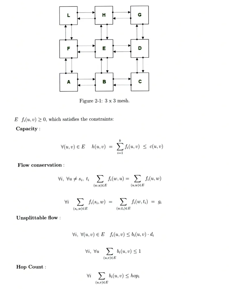
Assume that we have an acyclic Cycle Dependency Graph (CDG) DA. We transform it into a flow network GA, where an edge (u, v) E E has capacity c(u, v). The capacities c(u, v) are the available bandwidths on the edge. There is a set of k data transfers or flows K = {Ki, K2, .. , Kk}. Ki = (si, ti, di), where si and ti are the

source and sink, respectively, for connection i, and di is the demand. We assume si 5 ti. We may have multiple flows with the same source and destination. The variable for flow i along edge (u, v) is fi(u, v). A route is a path pi from si to ti for a flow i. Edges along this path will have fi(u, v) > 0, other edges will have fi(u, v) = 0. The capacity of an edge in GA is the capacity of the link/vertex that the edge is incident on. For example, the edge from si to AB will be assigned the capacity of link/vertex AB. An edge from AB to BC will be assigned the capacity associated with link/vertex BC. Edges into destination nodes di have infinite capacity.

Figure 2-1: 3 x 3 mesh.

E fi(u, v) > O, which satisfies the constraints:

Capacity :

V(u, v) E E

k

h(u, v) =

f(u, v) < c(u, v)

Flow conservation:

$

Sf,

_{(, ) =}

Vi

x

f,(si,w)

=

Unsplittable flow :

Vi, V(u, v) e E

Hop Count:

Vi

I

b (u,v) < hopi

E

and maximizes the total throughput, given as

maximize S = gi (2.1)

i=1

or maximizes the minimal fraction of the flow of each commodity to its demand:

maximize T

min

(2.2)

1<i<k di

or minimizes the maximum channel load:

minimize U = max h(u, v) (2.3)

(u,v)EE

The variables bi(u, v) are Boolean variables, i.e., they can take on values of 0 or 1 only. They enforce the restriction that a flow i can only take a single path from source si to destination ti. Path length restrictions are also enforced. hopi is a specified constant that can be set to be equal to the minimal path length between si and ti. This will imply that only minimal paths will be considered. hopi should be incremented by 2 or more to allow for non-minimal routing. The fi(u, v) variables can take on any positive value less than or equal to the demand di.

Even though the MILP formulation produces routes with unsplittable flows, the time it takes to compute grows exponentially as the problem size increases. Fur-thermore, even though there are various cost functions that have been formulated, a route with the highest throughput (Equation 2.1), or the biggest minimal fraction of each flow (Equation 2.2), or the lowest possible MCL (Equation 2.3), may not be the optimal route for performance. We would therefore like to find a polynomial-time algorithm that can find a set of routes with unsplittable flows that produce optimal performance.

Chapter 3

Routing Using Dijkstra's algorithm

XY and YX routings are minimal and deterministic, but are purely based on the source and destination positions and do not take into account network traffic infor-mation. If we could profile the applications before running and record bandwidth requirements for each source-destination pair, we could utilize this information in our routing algorithm, and thus generate better routes. This chapter proposes an oblivious routing algorithm based on Dijkstra's Algorithm for finding shortest paths. It provides a polynomial-time heuristic solution to the routing problem given knowl-edge of each flows bandwidth requirement. Since the routing algorithm is oblivious, very little hardware support is needed from the routers. Simple router designs that support source routing or node-table routing will do.

Traditionally Dijkstra's Algorithm is used to find the shortest paths from one source to all destinations on a directed graph. We can model the processing elements in diastolic arrays in [3] as nodes and the connections between processing elements as edges on our directed graph. If we set the weights on the edges to reflect the residual capacity of each link, we can then run Dijkstra's Algorithm to find the paths with the lowest weight. This way, congested links are avoided and the resulting graph would have many links with large residual capacities, and therefore is likely to perform well under high traffic loads. This chapter describes the implementation of the oblivious routing algorithm.

3.1

Dijkstra's Routing Algorithm

Dijkstra's algorithm for finding shortest paths is described in [7]. It solves the

single-source shortest path problem on a weighted, directed graph, where all edge weights

are non-negative.

Ideally we would like to have routes that avoid using links with little residual

capacity, so the network does not get congested. We can incorporate this idea by

using residual capacity information to modify the weights on the graph's edges. When

the residual capacity is high, the weight is small and when a link is heavily used, its

weight is increased. This modified Dijkstra's algorithm to find shortest paths for

routing is named Dijkstra's Routing Algorithm. Dijkstra's Routing Algorithm is less

liable to choose paths utilizing congested links as these edges have higher weights.

The idea is that Dijkstra's Routing Algorithm can give us a route with low congestion

by taking into account of bandwidth demands of each source-destination pair, and

will therefore perform better than the deterministic routing algorithms, XY and YX.

The complexity of the algorithm depends upon the implementation of the heap.

Here we chose a Fibonacci heap over an array or a binary min-heap for performance

reasons. If V is the number of vertices and E is the number of edges in the graph,

the complexity of extractmin for a Fibonacci heap is O(log V), and the complexity

of decreasekey is ((1).

Therefore, the complexity of Dijkstra's algorithm before

any modifications is O(V x extract-min + E x decreaseley) = O(V log V + E).

3.2

Setting the Weights

Dijkstra's algorithm is able to find paths with minimum weights from a source to

all destinations on the graph, given that all weights are non-negative. In order to incorporate Dijkstra's algorithm into our bandwidth sensitive routing, we have to modify the weights to not only take into account of the length of the path, but also its bandwidth demand.

We run Dijkstra's algorithm on a weighted, directed graph, deriving the weights from the residual capacities of each link. Consider a link e that has a capacity c(e). We create a variable for the link a(e) which is the current residual capacity of link e. Initially, it is equal to the capacity c(e) set to be a constant C. If a flow i is routed through this link e, we will subtract the demand di from the residual capacity. The residual capacity is always checked to see whether it is enough to supply the demand for the flow during routing. If there is not enough capacity, then Dijkstra's Routing Algorithm sets the weight of the link to be extremely high, so it never chooses the link. Therefore, the residual capacity c(e) will never be negative.

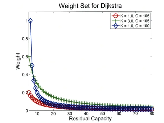
We have experimented with multiple ways of setting the weights. To take band-width into account, we decided to set the weight to be the reciprocal of link resid-ual capacity, similar to the CSPF metric described in [30]. Our weight function is (e) = ( except if c(e) < di, then w(e) = oc, and the algorithm never chooses the link. The constant C is set to be the smallest number that can provide us with routes for all flows without using oc-weight links. The maximum channel load (MCL)1 from XY or YX routing gives us an upper bound for C, but in most cases, we can set C lower and still find a solution. We want to set C lower because a lower C makes the algorithm more aggressively avoid congested links due to their higher weight. As it is shown in Figure 3-1, the weight function indicated by the line with diamonds has a lower C than the weight function indicated by the line with circles. We can see that links with lower residual capacity are punished even more on the line with diamonds as more effort is put into avoiding congested links. The Mixed Integer-Linear

Pro-1

MCL stands for Maximum Channel Load. This number is the maximum of link load for all

gramming (MILP) approach for routing presented in Section 2.4.1 generates routes

by setting the unsplittable flow constraint and minimizing MCL. The result given

by MILP sets a lower bound for C, but the routes do not necessarily perform the

best. C needs to be tuned along with K to get good results. K is a constant in the

weight function. The higher we set K, the more effort is put into minimizing the hop

count. As shown in Figure 3-1, the line with crosses shows a K value that is 3 times

the original K shown by the line with circles. The weight increases for every case

of residual capacity E(e). By setting higher weights corresponding to each c(e), we

effectively reduce hop counts and get shorter paths.

Weight Set for Dijkstra

- K= K 1.0, = 105 1 K =3.0, C= 105 K = 1.0, C= 100 0.8

Residual Capacity

Figure 3-1: Two weight functions over residual capacity

From the above paragraph, we conclude that by tweaking C and K in the weight

function, we set a trade-off between path length and link load. However, it is not

the case that the more weight we give to the more congested links, the better. If we

punish the congested links too much by setting C lower, the weights get extremely

high for links with low residual capacity. Figure 3-1 shows the line with diamonds

having much higher weights than the line with crosses for low residual capacities.

If this line with diamonds gets too high for low

a(e),

the weights are too high for

congested links then they matter so much that slightly less congested links do not

matter any more. We do not have any most congested links. However, this situation

is not as good as it first looks. We may still get many heavily congested links, despite

getting none of the most congested ones. Caution needs to be taken when setting C

and K in order to get a close to optimal solution.

3.3

_{Breaking Cycles Using the Turn Model}

Dijkstra's Routing Algorithm guarantees us the shortest weight path for each source to destination pair. However, it doesn't guarantee us a cycle free route. Cyclic routes may result in deadlock.

In a 2-D mesh, there are 8 possible 90-degree turns. XY and YX routes do not have deadlock problems because each of them only uses 4 of the 8 90-degree turns. Furthermore, the 4 turns used are such that there is no way a cycle can be formed using them. However, XY and YX routes may be too restrictive.

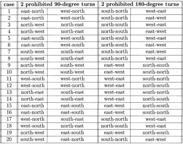
The turn model introduced in [11] only eliminates 2 of the 8 90-degree turns to eliminate cycles. If we assume that the mesh does not have wraparound channels and 0-degree turns, then we can also allow 2 out of the 4 180-degree turns. These turns to be eliminated are not random. As long as we follow the rules described in the turn model, we are guaranteed to get an acyclic set of routes which are thus deadlock-free. Enumeration of the turn model is listed in Table 3.1.

Allowing 2 out of 4 180-degree turns is merely for completeness of the turn model. Incorporating 180-degree turns does not produce better routes. If a 180-degree turn is chosen, it only adds extra path length. Since Dijkstra's Routing Algorithm tries to reduce each link's weight, which takes into account of hop count, 180-degree turns never appear in the routes produced.

There are two ways to generate acyclic routes. The first is to generate an acyclic CDG using the turn model, and then run the routing algorithm on it. Generating an acyclic CDG is described in [15]. The second way is to run Dijkstra's Routing Algorithm straight on the mesh. However, during execution we keep track of the direction of the incoming edge, aka, the parent of the node, and so we know which turn is being made for each outgoing edge. If that turn is not allowed in a specific turn model, then we set the weight on the illegal output edge to be very high; higher than any valid route. In doing this we make sure Dijkstra's Routing Algorithm will never choose to relax this edge and never choose this turn.

case

2 prohibited 90-degree turns 2 prohibited 180-degree turns

1 east-north west-north south-north west-east 2 east-north west-north south-north east-west 3 north-west north-east north-south west-east 4 north-west north-east north-south east-west 5 east-south west-south north-south west-east 6 east-south west-south north-south east-west 7 south-west south-east south-north east-west 8 south-west south-east south-north west-east 9 north-west south-west east-west north-south 10 north-west south-west east-west south-north 11 west-south west-north west-east south-north 12 west-south west-north west-east north-south 13 north-east south-east west-east south-north 14 north-east south-east west-east north-south 15 east-north east-south east-west north-south 16 east-north east-south east-west south-north 17 west-north south-east south-north west-east 18 west-south north-east north-south west-east 19 north-west east-south east-west north-south 20 south-west east-north south-north east-west

Table 3.1: Turns prohibited for 20 cases in the turn model

check. Parents of nodes are already tracked in the original Dijkstra's algorithm for finding shortest paths. Comparing the relative positions of nodes to determine whether they satisfy a particular turn model is an 0(1) computation. Therefore, the order of growth of our modified algorithm remains the same: O(V log V + E).

3.4

Nodes With 4 States

Dijkstra's Algorithm guarantees finding the shortest path from source to a particular

node after it extracts the node from the heap and finishes the Relax step. After it is

done with one node, it never goes back to relax the same node again. However, after

incorporating the turn model constraint, the current Dijkstra's Routing Algorithm

may not produce the correct shortest path, or a path at all when it should.

iS

1

"50

1

i

1*

D

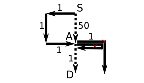
Figure 3-2: A situation where the current Dijkstra's Routing Algorithm would not

produce the correct answer.

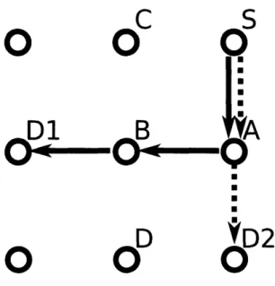
Consider the situation shown in Figure 3-2. We are trying to route from source S

to destination D. Going into node A, our current algorithm would pick the solid path

versus the dotted path, as it has the shortest distance of 3, versus the dotted path's

distance of 50. However, if we are using turn model case 15 or 16 shown in Table

3.1, east-north, east-south, and east-west turns are not allowed. Therefore, the solid

path cannot go south at node A because it cannot take an east-south turn. It can

only go east. After choosing the link with load 1 after node A, the solid path still

cannot go south because the east-south turn is prohibited. It can't go west either,

because the east-west turn is prohibited. Therefore, the solid path is a dead-end and

can never reach node D. Our current Dijkstra's Routing Algorithm would not produce

a valid route. However, in this case, the dotted path from S to A to D should have

been chosen. It is a valid route with weight 50 + 1 =

51, but the dotted path had

already been eliminated at node A. One way to solve this problem is to create four

nodes for each original node in our Dijkstra's Routing Algorithm. These new nodes

represent incoming edges from four different directions. In this case, at node A, there

is a state for the dotted path coming from the north AN and a state for the solid path

coming from the west Aw. Neither of them is thrown away at Node A because they

are distinct nodes. Both need to be relaxed and kept. Therefore, the correct shortest

path, which is the dotted path, will be found. Nodes that do not have incoming edges

from a particular direction will never be reached, but this doesn't pose a problem.

The algorithm would ignore those nodes and never try to extract them from the heap.

Dijkstra's Routing Algorithm is modified as described above. In the worst case,

there are 4 times as many nodes and edges to explore. The complexity of Dijkstra's

Routing Algorithm after this modification stays the same.

3.5

Modified Dijkstra: 1 Iteration vs. 100

Itera-tions

Our current Dijkstra's Routing Algorithm starts by routing the first source to

des-tination pair. The residual capacities are then modified and the weights updated. Then it routes the second source to destination pair with the modified weights which are based on the routing result of the first source to destination pair. Next it routes for the third source to destination pair using weights modified by the first two flows and so on.

The problem with this is that based on the order chosen to route source to desti-nation pair, the results can differ significantly. Consider the situation shown in Figure 3-3. The first pair is routed from S to D1 and the path chosen is shown by the solid arrows. The second pair from S to D2 is routed after the first and takes the path shown by the dotted arrows. In this case, S # A is congested, but S = A > D2 gives

the shortest path, because going around to S = C = B == D r= D2 is too expensive.

We would like to avoid this situation because we create a heavily congested edge between S and A.

od

S

D1

B

A

OC--

O*--D

D2

If we routed the S to D2 pair first, then S = A = D2 would be the path chosen as shown in Figure 3-4 by the dotted arrows. Then routing S to D1 Dijkstra's algorithm would be able to find a route that is less congested, but with the same number of hops: S = C = B = D1. As shown clearly in the example, routing order does matter.

0

C

S

O9

D1

B

A

o

D

VD2

Figure 3-4: Routing result for routing S to D2 first

The 100 iteration Dijkstra's Routing Algorithm tries to mitigate the effects caused by routing order. The idea is to route each pair many times growing the bandwidth requirements gradually. This would mean when we come to last iteration the first pair is routed onto a graph where the edge weights are nearly at their final values. In this way no flow is given the luxury of having been routed onto an empty mesh which caused the problem above. The algorithm works as follows: At iteration 1, we route all source to destination pairs with only 1 of each pair's flow demand. At iteration 2, we first erase the route for the first source to destination pair and reroute this flow with 2 of its demand. During this second routing process, a small amount of all other flows are on the mesh so the edge weights are affected by them, but their contribution is small, as only 1 of the demand for each flow has been routed. Then we erase and reroute the second source to destination pair, the third, and so on, with

2 _{of its flow demand. On the third iteration, we reroute each flow with I of its}

100demand, and so on. On iteration 100, we reroute with the full flow demand for all the

source to destination pairs with 2 of the flow demand for all other flows already on

the mesh. This algorithm reduces the effect caused by routing order. For the example

given above, the 100 iteration Dijkstra's Routing Algorithm is able to find the routes

shown in Figure 3-4 even though S -= D1 is routed first.

This algorithm essentially repeats the previous Dijkstra's Routing Algorithm 100

times. Erasing each path requires modifying the weights of all the edges that were

routed in the last iteration, and is an O(1) operation. The complexity of the algorithm

remains the same, though it takes 100 times more time than the original algorithm.

3.6

Output Selection Process

Dijkstra's Routing Algorithm produces routes by avoiding congested links at different

levels. The more congested the link is, the less likely Dijkstra's Routing Algorithm will

use that link as part of a route. Given a set of values for C and K, we run Dijkstra's

Routing Algorithm as described in this chapter, taking into consideration all 20 turn

model cases listed in Table 3.1. We reduce C from the MCL produced by XY to

the MCL produced by MILP presented in Section 2.4.1 or until we cannot obtain a

set of routes, storing the routes obtained for each value of C. Often times we have

several routes with the same MCL. We pick the set of routes with the least congestion

amongst all computed routes with the lowest MCL. Congestion corresponds to the

product of the average excess bandwidth demand over all links times the average

number of flows competing for each link.

We developed 2 relevant metrics we can use to analyze the results.

*

where n is the total

number of links that are used. This parameter is calculated by summing up

link load for all links, and then dividing the sum by the number of links in the

network. ACL reflects how congested the network traffic is.

*

Average Flow Competition Per VC (AFC)

where

n is the total number of virtual channels that are assigned flows to in the

net-work. This parameter is calculated by computing all the flows going into every

virtual channel, and then averaging it over all the virtual channels. AFC reflects

head-of-line blocking.

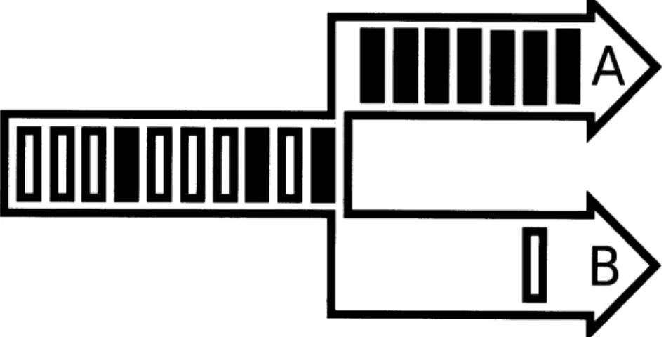
One case of head-of-line blocking is illustrated in Figure 3-5. There are two flows,

depicted as A and B in Figure 3-5, sharing the same link. Ahead of flow A, the traffic

is heavy and that part of the network is very congested. A cannot move because the

flow is congested. At the same time, there is almost no traffic ahead of the other flow

B. B should be able to move freely. However, B cannot move either, because A and B

2

VC stands for virtual channel. Each link in our mesh network has four virtual channels, each for one direction.

packets are interleaved, thus flow A is blocking flow B. The bigger the AFC, the more potential there is for head-of-line blocking.

From the above two network parameters, congestion is calculated as congestion

= (ACL -_{Threshold) x (AFC). Threshold is a parameter we can set. It can be thought}

of as the link capacity of the network. (ACL -Threshold) gives us the average excess bandwidth demand. This number multiplied with AFC, which is the potential for head-of-line blocking, gives us the congestion number.

We calculate this congestion number for all generated routes with the lowest MCL, and pick the route with the lowest congestion number.

fOB

Figure 3-5: Head-of-line blocking illustration. There is heavy congestion ahead of flow A, and no congestion ahead of flow B after the split.

Chapter 4

Experiments with Dijkstra's

Routing Algorithm

As described in Chapter 3, the complexity of Dijkstra's Routing Algorithm is 8(V log V+ E), which is polynomial. Dimension-order routings like XY and YX are simple algo-rithms which take linear time to route, but they may not give good routing results because the bandwidth demand of each route is not taken into account.

This chapter details the simulator and simulation method we use to measure the performance in Section 4.1. Section 4.2.1 evaluates the actual performance when compared with DOR (dimension-order routing) and maximum channel load results compared with ROMM and Valiant. The analysis for the simulation results is dis-cussed in Section 4.2.2.

4.1

Simulation Process

4.1.1

The Simulator

A cycle-accurate network simulator is used to estimate the throughput and latency of

each flow in the application for various oblivious routing algorithms. The simulator models the router micro-architecture with four stages. As discussed in Section 2.3, our routing scheme only requires minor changes in modern router hardware design. Therefore, we assume an identical clock frequency for all routing algorithms.

We use an 8 x 8 2-D mesh network with 1 to 8 virtual channels per port. The simulator is configured to have a per-hop latency of 1 cycle, and 16 flits of buffer size per VC. We simulate a fixed packet length of 8 flits. For each simulation, the network is warmed up for 20,000 cycles prior to being measured, after which the simulation is run for 100,000 cycles to collect statistics. This is enough for convergence.

We vary the input injection rate and measure the throughput of the network. A high throughput under a high input injection rate for a specific set of routes shows that the routes perform better. When the input injection rate is low, the throughput should converge to the same value, dominated and controlled by the injection rate of the input. When the input injection rate is moderate, the network is reasonably congested. A better route with a lower MCL with little head-of-line blocking should produce a higher throughput.

Input injection rates are tuned so that the maximum transmission rates of the network would cover the range in between the MCLs of the two routes being compared. Any difference in performance between two routes should be most visible within this region. Above this region both networks are congested, whereas below neither would be. Only within this region should the set of routes with a lower MCL not be congested while the other set is.

4.1.2

Benchmarks

We use a set of standard synthetic traffic patterns, namely transpose, bit-complement, and shuffle in our experiments. They are defined as follows:

* bitcomp: di = si

* shuffle: di = Si-1 mod b

* transpose: di = Si+b modb

where si(di) denotes the ith bit of the source (destination) address.

The bit length of an address is b = log₂ N, where N is the number of nodes in the network. The synthetic benchmarks provide basic comparisons between Dijkstra's Routing Algorithm and other oblivious routing algorithms, since they are widely used to evaluate routing algorithms. In the above three synthetic benchmarks, all flows have the same average bandwidth demands. We also report results on H.264, which is a widely known and used application. We profiled a 4-engine H.264 decoder and recorded all the flows' demands. This benchmark exhibits significantly varying flow demands - by up to 2 orders of magnitude. It is usually the case that different applications have vastly different flow demands.

4.2

Performance Evaluation of Dijkstra's Algorithm

4.2.1

Channel Load Comparison

The following table 4.1 shows the MCL computed by each routing algorithm.

Traffic

XY

YX

ROMM Valiant

Dijkstra's Routing Algorithm

transpose

175

175

200

175

75

bit-complement

100

100

400

200

100

shuffle

100

100

150

200

75

H.264

214.48 365.51

336.14

352.98

124.54

Table 4.1: Comparison of Maximum Channel Load (MCL) in MB/second.

As shown, Dijkstra's Routing Algorithm always finds routes with as low an, or

lower, MCL compared with XY/YX, ROMM, and Valiant routings. Dijkstra's

Rout-ing Algorithm finds the same lowest MCL as XY/YX for bit-complement. This is

because the flows in bit-complement have many source and destination positions

across the mesh, making it highly symmetric both in the x and y direction.

Fig-ure 4-1 shows the bandwidth demand for each flow and the routes determined by

Dijkstra's Routing Algorithm for bit-complement. Each arrow represents a unit of

flow demand. The more arrows pointing to the same direction on a link, the more

congested the link is in that direction. The symmetry of the benchmark is clearly

seen. For comparison, the same plot is generated for transpose, shown in Figure 4-2.

There is not as much symmetry in this figure. For the case of bit-complement, this

symmetry makes a minimal and deterministic routing algorithm, XY/YX, attractive

for this particular traffic pattern.

However, Dijkstra's Routing Algorithm finds the same result as XY/YX for

bit-complement, which shows its generality. Dijkstra's Routing Algorithm produces

routes with the same or lower MCL than XY/YX.

In this thesis, ROMM and Valiant have been implemented to randomly choose an

intermediate point on a per-flow basis, not a per-packet basis. They both produce

routes that have higher MCLs than XY/YX for the three synthetic benchmarks. The

three synthetic benchmarks that we use have relatively symmetric traffic patterns,

which make XY or YX attractive. Even though ROMM and Valiant add randomness

into the network to balance the load, the MCLs of the routes produced by ROMM and

Valiant are higher than routes produced by XY/YX for bit-complement, transpose

and shuffle. It should be noted that this is not the case for H.264.

Figure 4-1: Routes generated using Dijkstra's Routing Algorithm for bit-complement.

4.2.2

_{Simulation Results of Four Synthetic Benchmarks}

Routes are produced by Dijkstra's Routing Algorithm on four benchmarks, discussed

in Section 4.1.2. Since there are 20 different turn models described in Section 3.3, there

are 20 results produced. The selection process described in Section 3.6 is used to pick the routes with the lowest MCL and the least congestion. It selects one set of routes for each benchmark. The threshold is set to be 25 for all four benchmarks. Figures 4-3 through 4-6 1 show the throughput corresponding to various input injection rates for Dijkstra's Routing Algorithm, XY, and YX on the four benchmarks. Offered injection rate is the injection rate per MB/s bandwidth.

As can be observed from Figures 4-3 through 4-6, Dijkstra's Routing Algorithm outperforms existing oblivious routing algorithms significantly in most of the bench-marks. This is seen in the reduction of the MCL and the number of congested links whose channel load is close to the MCL. Figures 4-4 and 4-5 clearly show that when the injection rate is low, the throughput is dominated by the injection rate. The throughput converges to the same value for all routing algorithms.

An interesting result to note is that of bit-complement. The best result is given by minimal routing, YX. This is because the flow demands in bit-complement are highly symmetric, as described in Section 4.2.1. This is the reason why YX routing would give us the lowest MCL, and thus a good simulation result. Dijkstra's Routing Algorithm was able to produce the same routes as XY or YX when XY/YX routes are optimal, in this instance.

The performance of Dijkstra's Routing Algorithm shown in Figure 4-6 for the H.264 benchmark, on the other hand, is better than XY/YX under moderate traffic shown in Figure 4-7. However, as the network gets congested, head-of-line blocking becomes more of an issue for the routes produced by Dijkstra's Routing Algorithm, because they become unstable. If the network capacity is restricted, the correlation between MCL and the performance of the routes diminishes, and we should instead focus on choosing the set of routes with the least head-of-line blocking to make sure they are stable. Figure 4-8 shows the performance of an alternative set of routes cho-sen from the 20 routes generated by Dijkstra's Routing Algorithm. This alternative set of routes has little head-of-line blocking, and thus they are stable and perform

1XY-1 is the performance of XY with 1 virtual channel, YX-2 is YX with 2 virtual channels and DJK-2 is Dijkstra's Routing Algorithm with 2 virtual channels, etc.

better than XY/YX for all input injection rates.

Bitcomp

2 4 6 8 10

Offered Injection Rate (packets/cycle)

Figure 4-3: Load-throughput graphs for bit-complement on a router with 1 or 2 VCs.

4.2.3

Simulation Result with Bandwidth Variations

The motivation for this experiment stems from the fact that the bandwidth profiling

is unlikely to be exact, and it is important to know whether the routes produced by

Dijkstra's Routing Algorithm are still robust enough to outperform DOR. Figure 4-9

shows the performance after the bandwidths have been varied. In this experiment, we

use the same routes as those used in Figure 4-4. The demands are, however, changed

to be between +10% to +50% of the original. For each flow, the bandwidth could

be as little as half or as much as 1.5 times as the original demand. It is clear that

Dijkstra's Routing Algorithm continues to outperform XY/YX because it spreads the

load across the network.

Transpose

0 2 4 6

Offered Injection Rate

8 10 12

(packets/cycle)

Figure 4-4: Load-throughput graphs for transpose on a router with 1 or 2 VCs.

Shuffle

Offered Injection Rate (packets/cycle)

H.264

-2

Offered

Injection

Rate (packets/cycle)

Figure 4-6: Load-throughput graphs for H.264 on a router with 1 or 2 VCs.

H.264

1

1.6

S1.2

_-

_XY-1

7

_-B-

_DJK-1

Offered Injection Rate (packets/cycle)

Figure 4-7: A zoomed in version of Figure 4-6 to show performance at low input injection rates.