Integration of Machine Vision and Virtual Reality for Computer-Assisted Micro Assembly

(1)

Publisher’s version / Version de l'éditeur:

Vous avez des questions? Nous pouvons vous aider. Pour communiquer directement avec un auteur, consultez la

première page de la revue dans laquelle son article a été publié afin de trouver ses coordonnées. Si vous n’arrivez pas à les repérer, communiquez avec nous à PublicationsArchive-ArchivesPublications@nrc-cnrc.gc.ca.

Questions? Contact the NRC Publications Archive team at

PublicationsArchive-ArchivesPublications@nrc-cnrc.gc.ca. If you wish to email the authors directly, please see the first page of the publication for their contact information.

https://publications-cnrc.canada.ca/fra/droits

L’accès à ce site Web et l’utilisation de son contenu sont assujettis aux conditions présentées dans le site LISEZ CES CONDITIONS ATTENTIVEMENT AVANT D’UTILISER CE SITE WEB.

Research Report (National Research Council of Canada. Institute for Research in Construction), 2007-12-01

READ THESE TERMS AND CONDITIONS CAREFULLY BEFORE USING THIS WEBSITE. https://nrc-publications.canada.ca/eng/copyright

NRC Publications Archive Record / Notice des Archives des publications du CNRC :

https://nrc-publications.canada.ca/eng/view/object/?id=46f1a099-78f4-4fc8-af20-400e0449d625 https://publications-cnrc.canada.ca/fra/voir/objet/?id=46f1a099-78f4-4fc8-af20-400e0449d625

NRC Publications Archive

Archives des publications du CNRC

For the publisher’s version, please access the DOI link below./ Pour consulter la version de l’éditeur, utilisez le lien DOI ci-dessous.

https://doi.org/10.4224/20378356

Access and use of this website and the material on it are subject to the Terms and Conditions set forth at

Integration of Machine Vision and Virtual Reality for Computer-Assisted Micro Assembly

(2)

http://irc.nrc-cnrc.gc.ca

I n t e g r a t i o n o f M a c h i n e V i s i o n a n d V i r t u a l

R e a l i t y f o r C o m p u t e r - A s s i s t e d M i c r o

A s s e m b l y

R R - 2 4 4

F a u c h r e a u , C . ; P a r d a s a n i , A . ; A h a m e d , S . ;

W o n g , B .

D e c e m b e r 2 0 0 7

The material in this document is covered by the provisions of the Copyright Act, by Canadian laws, policies, regulations and international agreements. Such provisions serve to identify the information source and, in specific instances, to prohibit reproduction of materials without written permission. For more information visit http://laws.justice.gc.ca/en/showtdm/cs/C-42

Les renseignements dans ce document sont protégés par la Loi sur le droit d'auteur, par les lois, les politiques et les règlements du Canada et des accords internationaux. Ces dispositions permettent d'identifier la source de l'information et, dans certains cas, d'interdire la copie de documents sans permission écrite. Pour obtenir de plus amples renseignements : http://lois.justice.gc.ca/fr/showtdm/cs/C-42

(3)

Integration of Machine Vision and Virtual Reality for

Computer-assisted Micro Assembly

ABSTRACT

The technical report describes the design and implementation of machine vision and virtual reality modules and their integration with the motion system of the in-house developed micro assembly system. Though the underlying techniques can be applied to a range of micro assembly scenarios, the demonstration of the techniques is applied for the “peg in a hole” assembly that involves operations such as picking pins from holes in a block and then subsequently inserting pins in desired locations in empty holes. The automation of pick and place operations requires addressing the issues of machine vision, sensing of position of holes and pins in a block.

The work described in this technical report is the continuation of the previous work to control motion system hardware through virtual reality interface and machine vision [PORCIN-RAUX, Pierre-Nicolas, Motion Control of Micro assembly System using Virtual Modeling and Machine Vision, Technical Report]. The current work advances the previous work of human-assisted pick and place procedure to achieve full automation of “peg in a hole” assembly.

The first part of this report describes technical issues that need to be addressed to achieve full automation of “peg in a hole” assembly. The alternative solutions are listed with all their advantages and drawbacks to help select the final solution. The second part explains the National Instruments LabVIEW® Virtual Interface (VI) and subVIs and describes how to execute the LabVIEW® application program. The last section of the document describes the procedure for creating and use of VRML model in a labVIEW® environment.

(4)

Table of Figures

Figure 1: Template tried for the pattern matching ...9

Figure 2: Same snap shot with a black and a white background ...10

Figure 3: Template used to find the block ...10

Figure 4: Image from the top camera before the processing ...11

Figure 5: Parameters of the image processing ...11

Figure 6: Processed image for use in the pattern matching...12

Figure 7: Template used to find the accurate position of the block ...12

Figure 8: Issues related to the pin recognition ...13

Figure 9: Position returned by labVIEW when it cannot find the correct matching ...14

Figure 10: Arrays for the position of the pins ...14

Figure 11: Gripper fully opened on top of a hole ...15

Figure 12: Cycle without collision issue (small angle) ...15

Figure 13: Cycle with a collision issue (angle bigger than 0.3rad) ...16

Figure 14: Collision issues pictures...16

Figure 15: Starting window of the NI Vision acquisition software...18

Figure 16: Acquisition board ...18

Figure 17: Camera choice...19

Figure 18: Image of the whole rotary table...19

Figure 19: Selecting “image calibration” in the “image” menu ...19

Figure 20: Selecting the type of calibration ...20

Figure 21: Changing the unit in mm for the calibration and choosing the center of the grid ...20

Figure 22: Specify calibration axis ...20

Figure 23: Specifying the user defined four other points...21

Figure 24: Saving the calibration file ...21

Figure 25: Overwrite the previous file if needed...22

Figure 26: Icon for step 1 ...24

Figure 27: Icon for step 2 ...25

Figure 28: Icons for the demonstration ...26

Figure 29: Loading every subVIs ...26

Figure 30: Tabs of the interface ...26

Figure 31: Icon for outputdrive_subVI ...27

Figure 32: Icon and initialization of the outputdrive subVI...28

Figure 33: Hiding parts from an assembly ...31

Figure 34: Base and x stage base to export in wrl ...31

Figure 35: Saving a SolidWorks part as wrl file...32

Figure 36: Checking the VRML options ...32

Figure 37: LabVIEW code to import VRML files...33

Figure 38: Result if the two VRML files have been created from two different files in SolidWorks ...33

Figure 39: Result if the two VRML files have been created from the same SolidWorks assembly...34

Figure 40: Origin issue for the rotary plate...35

Figure 41: Open a part from an assembly...35

(6)

Figure 43: SolidWorks measurements ...36

Figure 44: How to match the offset in labVIEW ...37

Figure 45: 3D scene of the bottom stages ...37

Figure 46: Calibration step 1 code ...38

Figure 47: SolidWorks measurement between the TCP and the center of the zoom lens...39

Figure 48: Calibration step 2 reading the first position ...39

Figure 49: Calibration step 2 reading the second position of Zaber and computing the transformation ...40

Figure 50: SolidWorks measurement of distance between the gripper and the rotary table. ...40

Figure 51: Initialization of the X and Y stages...41

Figure 52: Initialization of the X,Y, and Rotary stages ...41

Figure 53: Updating the position of the virtual model of X stage...43

Figure 54: Updating the rotary table...43

Figure 55: Updating the whole VRML model ...44

Figure 56: Creating the motions...44

Figure 57: Main VI part 1 ...52

Figure 60: Main VI part4 ...53

Figure 61: Main VI part5 ...54

Figure 63: Aerotech stages control ...55

Figure 64: VRML importation and update ...55

Figure 65: Link between the hardware stages and the virtual stages ...56

(7)

Table of Appendix

APPENDIX A: Calibration of the system ...46

APPENDIX B: Main VI ...52

APPENDIX C: Find block...57

APPENDIX D: Find the holes...59

(8)

1 Introduction

The trend and growing demand for the miniaturization of industrial and consumer products has resulted in an urgent need for assembly technologies to support economical methods to produce micro systems in large quantities. More powerful, next generation micro systems will consist of a combination of sensors, actuators, mechanical parts, computation and communication subsystems in one package. This will require significant research and development of new methods for transporting, gripping, positioning, aligning, fixturing and joining of micro components.

In response, a team at NRC-IMTI began an initiative to develop computer-assisted assembly processes and a production system for the assembly of micro systems. Since 2005, the project team has designed, assembled, and calibrated an experimental test system for the precision assembly of micro-devices. The system makes use of high precision motion stages, micromanipulators, grippers, and the machine vision system to develop a platform for computer assisted assembly of Microsystems [5.1]. Examples of Microsystems that the production system is aimed to assemble are: pumps, motors, actuators, sensors and medical devices.

The basic operations in an automated assembly involve picking, moving, and mating relevant parts. To develop software modules that can be reused for other applications (e.g. assembly of micro pumps, actuators, etc.), a simple “peg in a hole” assembly problem was chosen. The problem scenario involves picking 210 micron pins from holes in a plastic block using a micro gripper and then placing it in another empty hole in the same block.

The following describes the control loop for the pick and place of 210 micron pins:

1. Start the execution of the program after placing the plastic block on the positioning table.

2. The user fills in a two dimensional array on the user interface to let the system know where the pins are and the destinations.

3. The system should find the exact location and 2D orientation of the plastic block:

3.1 The machine vision system finds the position and 2D orientation of the plastic block on the positioning table. The image analyses of the picture taken by the global camera computes the location of the block. The location thus obtained is an approximate location but good enough for the next step of finding the exact location of the holes. This position information is then used to place the VRML model of the block in 3D space.

3.2. Now that the approximate location of the block on the rotary plate is known, the block is to be brought under the objective of the vertical zoom lens.

(9)

The motion system is commanded to lift the micro gripper up to the clearance plane. It is then commanded to move over the pick position.

4. Open Gripper

The gripper is commanded to open, and advance towards the pin keeping centre of the opened jaw aimed at the pin.

5. Lower the Gripper: the gripper is commanded to lower to the Working Plane.

6. Grip the pin: the gripper is commanded to close when the pin is at the centre of the open gripper.

7. Lift the gripper to the Clearance Plane.

8. Move the pin to the desired hole: The motion system commands the gripper to go to the pre-calculated location of the hole on the block.

9. Release the pin by opening the gripper

10. The same operations are followed for the second pin and then the process is reversed to put the pins back.

Above is the architecture of the micro assembly system built at NRC London to achieve the assembly of microsystems. The components that play a key role in the assembly process are pointed to on the picture.

Automating all these steps require numerous issues to be solved for the “peg in a hole” example to have consistent results. Finding the position and orientation of the block through the vision system is described in Section 2. The accuracy of measurements of the machine vision system depends on accurate calibration. The method for machine vision calibration is described in Section 2.1.4

High magnification images from the zoom lenses suffer from very low depth perception. Therefore to assist users in the handling of parts, a virtual reality model of the system has been created to visualize the system in 3D. This virtual model is synchronized to the motion system to provide good feedback. The virtual model is integrated with the motion system through the position information obtained through machine vision and displacement sensors on the motion system as described in Section 4.

(10)

2 Machine vision assisted automated pick and place

2.1 Finding the parts and their orientation

At a micro level, finding parts with their orientation is a tough challenge due to the geometry and accuracies required. Machine vision is used to locate parts on the rotary table. Two steps are needed to get the highest accuracy on the part location and orientation. The first step is that of finding the position of the block on the positioning table and the second step involves finding the position of the holes on the block. Pattern and geometry matching were used to find the position of the parts.

2.1.1 Finding the position of the block

Pattern matching relies on the uniqueness of the template. Therefore, either a unique shape or color contrast that can be easily recognized is earmarked as a template.

Different templates (with various shapes and colors (see Figure 1) were tried to find out which one was the best. ”The best” here implies that the machine vision will find it repeatedly wherever it is located on the positioning table without any errors.

Figure 1: Template tried for the pattern matching

During the testing of different templates, the issue of illumination was found to be a very important variable. At the micro level, adequate and the right type of illumination is very important. Even if the light intensity is varied slightly, the machine vision will not be able to find the template consistently.

Through experiments we observed that the color pattern matching was not a good solution because the illumination greatly influences the results. Moreover, the system uses black and white cameras. To obtain a color image, cameras were calibrated with Bayer filters. But this calibration is probably not accurate enough to obtain the best results. Even having the same intensity of light, the recognition did not yield similar results each time. But for a fully automated cycle, the recognition must work every single time without human intervention.

(11)

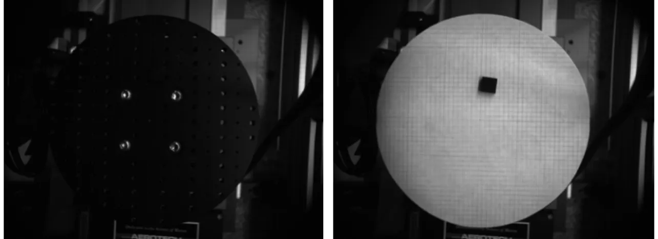
Due to the black color of both the block and the table, it is hard to find the block with the machine vision system. To distinguish the block on the rotary table, greater contrast between these two parts was needed. Placing white, blank paper on the rotary table improved the contrast significantly. (Figure 2).

Another advantage of the black and white image is that the light intensity is less important than it is for the color image allowing small variations in illumination which improves the flexibility of the system.

A sharp black and white image is obtained by fine tuning the software-based camera parameters such as frames per second and by adjusting the focus and aperture rings manually. Further, if needed, the Image Acquisition software from National Instruments allows users to change a number of parameters such as contrast, brightness and to process the images.

By adjusting the parameters, a clear image is obtained with the block easily recognizable on the table. Using this image (Figure 3) as a template, the pattern matching combined with geometry matching can find the position of the block.

Figure 2: Same snap shot with a black and a white background

Figure 3: Template used to find the block

If the global camera has been properly calibrated (see section 2.1.4), the machine vision system computes the location of the block which is used in the next step by bringing the block under the zoom lens such that all holes are visible.

(12)

2.1.2 Finding the accurate position of the block

Mostly, due to the small size of the parts, a location error of less than half a millimeter from the global camera is acceptable [5.2]. For the positional higher accuracy, the top zoom lens camera system, which has very high magnification capability, is used. After having brought the block under the zoom lens (by using the position returned by the global camera), the exact location of the block and the holes are found using the pattern matching algorithm.

Before the image is processed, its contrast and brightness is adjusted such that it will yield consistent results when processed.

Figure 4: Image from the top camera before the processing

Starting from Figure 4, and changing parameters such as contrast and brightness (Figure 5) an image, which can be used in pattern matching, was created (Figure 6). This image has also been used to create the template (Figure 7) for pattern matching.

Figure 5: Parameters of the image processing

(13)

Figure 6: Processed image for use in pattern matching

Figure 7: Template used to find the accurate position of the block

The template is processed by the pattern matching algorithm to find the exact location of the block and its angle. The angle can be found with the aid of the mark on the block.

This step of finding the exact location of the block and its angle is dependent on the previous step of bringing the block under the zoom lens. If the block is not properly brought under the zoom lens, (so that all holes are visible in the image) the matching may not work. That is why accurate calibration of the global camera is very important and a calibration method has been developed to do so (see section 1.1.4). Pattern matching using the template is a very powerful tool to address this issue.

(14)

2.1.3 Picking and placing the pins

After the exact location of the block is known, finding the pins in a fully automated way is the next step. Pattern matching has been tried but the recognitions did not yield consistent results each time. Most of the time the system was able to find the pins but not all of them. Geometric matching and shape recognition have been tried as well without consistent results.

The main reason is that it is hard to obtain a unique image that can be easily found by the system. When the pin is fully vertical in the hole, there is a gap between the hole’s edge and the pin’s edge (Figure 8). In this case the pin can be found by geometry or shape recognition because the white circle can be easily extracted from the black background.

But, on the other hand, if there is no gap between the hole and the pin’s edges, the vision system will not be able to recognize it (Figure 8). It is not a well defined circle anymore because of the white background around the holes.

Figure 8: Issues related to the pin recognition

So, if the matching doesn’t work correctly the system will find holes where there are none or completely miss an existing hole. Moreover, when the pattern recognition fails, labVIEW® returns to the original image (Figure 9) with the wrong holes positions.

Pin with a gap between the hole and itself.

Pin stuck to the hole’s border.

(15)

Figure 9: Position returned by labVIEW® when it cannot find the correct matching

As a first step in the process, the user input is required to indicate the initial location of the pins and their destination. Two arrays are used to ask the user where the pins are located in the block and where the user wants the pins to go as shown in Figure 10.

Figure 10: Arrays for the position of the pins

One of the developed main programs “run_demo_finding_pins_w_matching.vi” finds the pin automatically but it lacks consistency. Its performance depends on the orientation and angle of the pins in the holes as explained earlier. These issues have been solved and the system is tuned to yield consistent results. With the input data of the arrays (Figure 10), combined with the accurate position of the block, the coordinates of every single pin and its destination can be computed.

The specific example of (peg in a hole) has posed several challenges. First, the holes are much bigger in diameter than the pins resulting in the pins not being perpendicular to the surface of the block. Thus grasping pins is a problem as the camera finds the location of the pin by looking at the top of the pin (as the circle). But due to the tilt of the pin, this computed position is different from the position where the gripper actually grasps the pin. Though the wide opening range of the gripper (Figure 11), helps resolve this problem, it creates a secondary problem by shifting the block. The solution of this issue is explained in 2.1.4.2.

Wrong position returned

(16)

Figure 11: Gripper fully opened on top of a hole

The other issue is about the system knowing which pin it has to pick up first. Actually, in several cases, if the choice of pin is wrong the gripper will most likely not be able to pick it up because it will collide with another pin. However, in the demonstration, the system deals with two pins only. The only criteria being that the block has to be perfectly perpendicular to the axis of the lens. If the perpendicularity is more than 0.1 rad collision issues will result.

Following sequence of images explain these collisions issues:

Step 1 Step 2 Step 3

Step 4 Step 5

(17)

Step 1: Original state of the block and the pins. Step 2: Moving the first pin.

Step 3: Moving the second pin. Step 4: Moving back pin number 2. Step 5: Moving back pin number 1.

With a large angle

Step 1 Step 2 Step 3

Step 4 Step 5

Figure 13: Cycle with a collision issue (angle bigger than 0.3rad)

When step 5 is reached, the gripper is not able to pick up the last pin. It will actually collide with the first pin (Figure 14). This can either bend the pin or damage the gripper.

(18)

This issue can be overcome by rotating the positioning plate. The magnitude of rotation would depend on the angle ot the block on the positioning table. It could be either 90 or 180 degrees. For this particular application, a control logic could have been added to choose the pin to be picked up first. But, it was chosen to not demonstrate the flexibility of the developed system. Different case studies were developed to demonstrate the capability of the system.

In the long term it could be interesting to design and manufacture a tool holder that could help overcome this issue. It could improve the flexibility of the system.

(19)

2.1.4 Fine tuning the machine vision system for accuracy As accuracy is crucial for the measurements and location of the parts a methodology has been developed for calibration of all cameras used in the system.

2.1.4.1 Calibration of the cameras

To obtain the highest accuracy from the machine vision system, careful calibration needs to be performed. For the top camera, see the report IMTI-CTR-189 (2006/10) by Alfred H.K. Sham [5.4].

For the global camera, the NI vision software is used for calibration. Following are the steps required in preparation for calibration of the global camera.

• Bring the rotary table to the position X=49 Y=49.

• Put the grid paper on, and then, run the Vision Assistant 8.5. • Click on Acquire Image (Figure 15)

Figure 15: Starting window of the NI Vision acquisition software

• Click on Acquire image from the selected camera and image acquisition board. (Figure 16)

Figure 16: Acquisition board

• Select the device NI PCI-1426 (img1) Channel 0 (Figure 17) • Start acquiring continuous images

(20)

Figure 17: Camera choice

• Adjust the zoom in the software to have the full image in the window

• Make sure that the camera has a full view of the positioning table, otherwise move the flexible shaft to get it. Adjust the focus and aperture of the camera manually (by turning the rings) for the sharpest image

Figure 18: Image of the whole rotary table

• Click on the Store Acquired Image button in the browser and close it.

If the image is not clear, adjust the brightness, contrast and gamma level values to obtain a good image.

The calibration procedure can now start as follows:

• Select the Image item from the menu bar and then select Image Calibration (Figure 19)

(21)

• In the screen shown in Figure 20 select “Calibration Using User Defined Points”

Figure 20: Selecting the type of calibration

• In the calibration set up window, select the millimeter unit in the drop down box (Figure 21)

Figure 21: Changing the unit in mm for the calibration and choosing the center of the grid

• Click on the center of the grid, zoom in if necessary. This point is also the center of the coordinates system, so in the real world it has (0, 0) coordinates. Write down the image coordinates

• Go to the “specify calibration axis” tab (Figure 22)

Figure 22: Specify calibration axis

• Enter the image coordinates as “user defined” value for “Axis Origin” (Figure 22)

• Change the direction of Axis Reference to have the same system of axis as defined in Aerotech motion stages. (Figure 22)

(22)

• Adjust the angle to have the red X axis parallel to the rotary plate’s axis. (Figure 22)

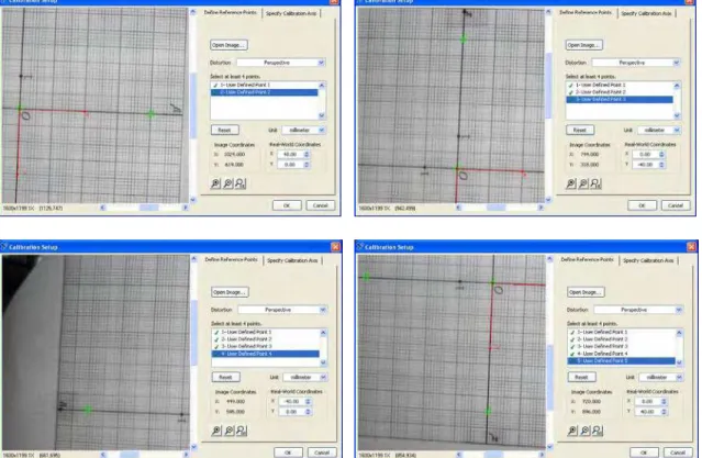
• Switch back to “Define reference points” tab

• Select four other points (as shown in the Figure 23) for which the exact coordinates are known. In Figure 22, the real world coordinates are 1: (0;0) 2: (40;0) 3: (0;-40) 4: (-40;0) 5: (0;40)

Figure 23: Specifying the user defined four other points

• Once done, press the OK button and save the image (in ___ folder as calibration_rotary_plate.png for example). (Figure 24) Overwrite the previous file if needed. (Figure 25)

(23)

Figure 25: Overwrite the previous file if needed

Usually, once cameras are calibrated the procedure does not need to be repeated unless camera position has changed. In our lab, the calibration procedure has to be repeated at least every week because the flexible shaft slightly drops every day. Since the accuracy of measurements will be dependent of these calibrations so it has to be done very well.

(24)

2.1.4.2 Keeping the accuracy along the cycle

As the pick and place cycle executes, picking a pin from a hole and dropping the pin in another hole, the block shifted due to reasons described in 2.1.3. When the block shifts, the gripper drops the pins slightly off the holes.

The issue was resolved by taking a new snap-shot each time the system is picking or dropping a pin. This way, it allows the system to compute the location of holes through pattern matching for each new step of the cycle. Thus, even if the block has shifted slightly its new position can be computed accurately. It slightly increases the cycle time but it is the most accurate way to overcome this block shifting issue. Another solution that we found useful was to mount the block on a thin sponge and then secure the sponge on the positioning table. If the pin is not at the centre of the gripper then the block will tilt slightly when the gripper closes but return to its position once the pin has been lifted out of the hole.

(25)

3 Procedure to run the demonstration

To turn the system on, follow the procedure as described in the document (Reference: IMTI-TR-036 (2007/01) Automated Assembly of Microsystems Start Up and Shut Down Procedures by Brian Wong [5.5])

All the VIs that are referred to in this report are located in the “Christophe” folder in the drive. A backup is also stored in the Christophe folder on G:\concurrent-eng\Microassembly drive.

3.1 Initializing the system

The first step is to calibrate the gripper. Two steps are needed to complete this task. These steps are also used to initialize the VRML model.

- Calibration_gripper_step1 (Figure 26) lets user locate the tool center point. It is the first part for the VRML initialization and finds the exact location of the gripper in relation to the centre of the positioning table. The location of the gripper is used in the main program.

Figure 26: Icon for the step 1

Before running the VI, make sure the gripper is in its folded position because every motion system axis is sent to its home position at the start of this VI. As soon as this initialization is completed the gripper fixture can be opened to its final position by tightening the screw. 1- Turn the ring light to its maximum level.

2- Run the VI

Run button

3- Follow the instructions on the user interface screen

4- When the new configuration file has been saved, stop the VI and exit.

(26)

- Calibration_gripper_step2 (Figure 27) is used to get the vertical distance of the gripper from the positioning table. Execution of this VI is for the VRML model initialization.

Figure 27: Icon for the step 2

1- Run the VI

Run button

2- Follow the instructions on the user interface screen

3- When the new configuration file has been saved, stop the VI and exit.

Stop button

These steps are not needed if the system has been run before. They have to be performed at each start of the system and each time the gripper is moved to a new position.

(27)

3.2 Running

the

demonstration

Open the run_demo_finding_pins_w_array VI or the run_demo_finding_pins_w_matching VI (Figure 28). The

run_demo_finding_pins_w_array VI lets the user enter the initial location and destination of pins. Whereas, run_demo_finding_pins_w_matching VI finds the initial location of pins leaving it up to the user to indicate the destination of the pins.

Figure 28: Icons for the demonstration

Wait till all VIs have been loaded correctly (Figure 29).

Figure 29: Loading every subVIs

Switch to the User_interface tab, (Figure 30) if not already done. Now, everything is ready to start the cycle.

Figure 30: Tabs of the interface

1- Run the VI

Run button

2- Wait till the VRML model is loaded (it takes approximately 30 seconds). The green light should turn off when the VRML has been loaded.

3- Make sure the ring light is at its minimum intensity. 4- Hit the “start cycle” button.

(28)

5- The motion system will first move the stages. The user interface asks the user to fill the arrays as shown in Figure 10. If the finding pin with array VI has been chosen there are two arrays (i.e. source and destination) to fill in. Otherwise, only one array (i.e. destination) has to be filled in. The, system then recognizes the block and finds its location. As soon as it has been done, the system brings the block under the zoom lens.

6- Turn the ring light to its maximum intensity.

7- The system recognizes the holes, the block center and the pins if the “finding pins with matching VI” is being run. The user only has to indicate the destinations for the pins in the graphical user interface.

8- The system computes the position of the holes.

Note: IF the position of the holes is not computed, then stop the VI by pressing the “STOP” button and re-start using step 1..

Stop button

9- The system will start the cycle of moving the pins.

If the cycle has to be stopped before its end, hit the Stop button:

Stop button

If the gripper is still open, open the “outputdrive_subvi” VI and run it (Figure 31). Wait till the gripper is closed and then stop the VI.

Figure 31: Icon for outputdrive_subVI

Note: When this VI is used (outputdrive_subvi), the gohomeatstart button needs to be activated before running the run_demo_finding_pins_w_array VI again.

(29)

3.3 Operating the “vacuum station” and the Gassmann

grippers

To generate the vacuum for the purpose of holding the parts or to generate mild air pressure to blow off the parts, open the “outputdrive_subvi” VI, run it and wait till the initialized system light turns on (Figure 32). Please refer to the section titled, “Festo Vacuum System” in “Automated Assembly of Microsystems Start Up and Shut Down Procedures”, Technical Report for layout of vacuum system.

Figure 32: Icon and initialization of the output drive subVI

The switches can then be activated to open and close the stop valves and the slider bars are used to control the vacuum regulation valve. Always turn on the Festo switch before activating the “air blow” or the vacuum. Make sure that the air blow (release pulse that generates the air pressure) and vacuum (vacuum generation) switches are NEVER turned on together. When the vacuum or air blow needs to be stopped, make sure that the slide is back to 0 and then hit Stop button.

Note: When this VI is used (outputdrive_subvi), the gohomeatstart button needs to be activated before running the run_demo_finding_pins_w_array VI again.

(30)

4 VRML models in labVIEW and its synchronization to

the motion system?

LabVIEW provides a few basic tools to manipulate 3D scenes. Careful thought on building the VRML model minimizes many of the selection and manipulation problems. This part of the documentation explains the steps to be followed to build a virtual model.

First, the section 4.1 explains how to build a VRML model in a way that allows for the motions we need, using two examples. Then, section 4.2 explains, the initialization procedure to make the VRML model interact with the hardware. Also, in the last part, how to build motions in the VRML model is explained.

4.1 Import files from SolidWorks to a 3D scene

Importing parts from SolidWorks® to labVIEW® through VRML may cause issues in linking and positioning parts in the 3D scene.

When a VRML file is created with SolidWorks, it retains the origin of the part as it was defined in SolidWorks®. Either, it is the origin of the assembly or the part itself (depending on whether the VRML file has been created from an assembly or a part file). When this file is imported in labVIEW® VI, it has its own origin and axis and it makes it coincident to the labVIEW and SolidWorks origin. Because these origins can be different, sometimes the parts need to be translated and rotated to synchronize the virtual and physical models. But, these transformations are constrained along the axis in labVIEW®. Other issues may also be found if relative motions between parts have to be set up as discussed in Section 3.

The front view in SolidWorks is used as a reference to describe the display orientation in LabVIEW®. This way you will know if the axis of the part has been built so that it can be used for the transformations in labVIEW®. So, while building the SolidWorks® model, the developer must exercise care in defining the origin of the part so that it will be the future axis of rotation and translation.

In order to limit the transformations, all VRML models, should be created from the whole assembly of the system in SolidWorks®. It can easily be done just by keeping the parts that have to be exported in VRMLand hiding all the other parts and then exporting the selected part. This way, each VRML file has the same origin, being “assembly”.

(31)

Also, to minimize the number of parts to import, all parts fixed together can be exported in the same file. The following are the assembly components used for this example:

- the base,

- the top stages base, - the x stage, - the y stage, - the u stage, - the xx stage, - the yy stage, - the zz stage,

- the moving parts of the gripper.

Figure 38 and Figure 39 illustrate why it is better to start from the whole assembly. But sometimes, parts need a special axis of rotation. In this case if the part itself has the origin needed, it is easy to open the part file and create the wrl file from this part. Otherwise it needs to be recreated with the right axis in SolidWorks. ®

(32)

4.1.1 Example 1: Importing the base and the x slide.

Figure 33: Hiding parts from an assembly

Hide all parts which are not needed by right clicking on the component name on the browser and hit Hide (Figure 33).

Figure 34: Base and x stage base to export in wrl

(33)

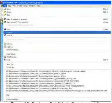
To export this part in a VRML format, go to file Save as (Figure 35)

Figure 35: Saving a SolidWorks® part as wrl file

Then, change the format following the step shown below (Figure 36).

Figure 36: Checking the VRML options

In the drop down

box select *.wrl Hit the option button, make sure the version is VRML97 and the length unit is set as meter.

(34)

Follow the above step for exporting the x slide. 2 files are finally obtained: the Base and the X slide.

In labVIEW® now, create a VI to import these 2 files. The Base has to be imported first and then, the x stage has to be added to the scene using an “invoke node” from the application palette (Figure 37).

Figure 37: LabVIEW code to import VRML files

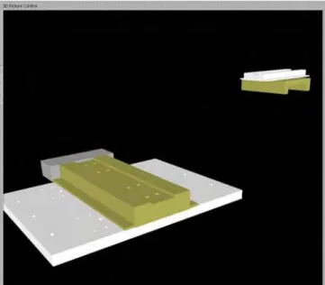
The following two figures (Figure 38, Figure 39) highlight the origin issue if the VRML files are created from two different SolidWorks® files. This illustrates why creating the files from the same assembly model is much easier.

(35)

Figure 39: Result if the two VRML files have been created from the same SolidWorks® assembly

This example was simple because there are no rotations and the translation axes remain the same in SolidWorks ®and labVIEW®.

(36)

4.1.2 Example 2: Importing the rotary table

If the same methodology is applied to import the rotary table model into the micro assembly system assembly model, another issue is raised because the origin of the system assembly is not at the center of the rotary plate (Figure 40). That means that if the rotary table is imported and a rotation has to be set up, the table is going to rotate around the assembly origin. Thus, a way to overcome this issue has to be found.

Figure 40: Origin issue for the rotary plate

Figure 41: Open a part from an assembly

Origin of the assembly

Origin of the rotary plate

(37)

Thus, a way to overcome this issue is found by setting up the model in such a way that the rotations have to be around the rotary plate origin. So the rotary table model has to be exported with its own origin from SolidWorks® and not the system origin. To do so, the part file can be opened in SolidWorks® by right clicking on to the file in the browser and selecting open part option from the pop-up menu as shown in Figure 41.

Figure 42: Rotary plate file with its origin

The origin of the part is in the center of the rotary plate and it has the same axis as that of the system assembly (Figure 42).

It can now be exported in *.wrl following the same steps as that of the previous example.

The next step is to define the offset of the origin of the system model from the origin of the rotary table in LabVIEW®. So, the distance measurement between the two origins has to be computed. This can be done using the measurement tool of SolidWorks as shown in Figure 43.

(38)

To import the VRML file in LabVIEW®, it is exactly the same procedure as in the previous example. The rotary plate has to be imported last, because it is the last part that is mounted on the lower motion stages (i.e. X and Y stages).

Figure 44: How to match the offset in labVIEW

The only difference from the previous example is that the origin of the system and the rotary plate has to be made co-incident by using a “Transformation Invoke” node from the Application Palette (Figure 44) of the LabView application. Be careful because the translation vector uses the metric units.

Figure 45: 3D scene of the bottom stages

The entire virtual model can now be built, importing each part or assembly. Offset

(39)

4.2 Initialize

the

model

To make the motion system hardware and the VRML model correspond to each other, several transformations need to be applied. To achieve the highest accuracy, the top camera is used to make the measurements of the distance between the gripper Tool Center Point (TCP) and the origin of the rotary table. In SolidWorks®, the measurement tool is used to make similar measurements. Once the gripper has been installed properly, the system is ready for the calibration. Two separate VIs have been created to get the position of the gripper with high accuracy. Once these VIs have been run, the data is stored in a configuration file which is used to update the 3D scene automatically in the main program. That means the calibration steps have to be done only when you re-install the gripper or disturb the location (i.e. fold it and put it back, for example).

4.2.1 Calibration step 1

Figure 46: Calibration step 1 code

Saving the data in a configuration file. Calculating the

offset between the TCP and the center of the image from top camera

Using the SolidWorks® measurements to compute the offset for translation to be applied to the VRML model

(40)

Figure 47: SolidWorks® measurement between the TCP and the center of the zoom lens.

4.2.2 Calibration step 2

The second step in the calibration process is to compute the height of the gripper from the rotary table. This is by finding the position of the Zaber® motion slide. Since the zoom lens is mounted on the Zaber® slide the position of the slide is an accurate measure of the position of the zoom lens. The working distance of the top camera is dependant on the focal length, hence it is fixed. Therefore, if the camera is focused first on the rotary table and then on the TCP of the gripper, the lower and upper positions of Zaber® slide are recorded (let us call them Z1 & Z2). Hence the height of the gripper from the rotary table, H = (Z1-Z2)

Figure 48: Calibration step 2 reading the first position

Reading the first position of Zaber slide (Z1)

(41)

Figure 49: Calibration step 2 reading the second position of Zaber® and computing the transformation

Figure 50: SolidWorks® measurement of distance between the gripper and the rotary table.

Reading the second position of Zaber® slide (Z2) and computing these values with the SolidWorks measurements to calculate the transformation to apply in the VRML model.

Then saving these values in the configuration file.

(42)

4.2.3 Import and initialization of the X, Y, and Rotary stages.

Figure 51: Initialization of the X and Y stages

Once all the files have been imported in LabView® for the X, Y, and Rotary motion stages, the transformations according to the configuration values have to be performed. To do so, the configuration file is read and then, the transformations are applied to the scene (Figure 51 and Figure 52).

Figure 52: Initialization of the X,Y, and Rotary stages

Reading of our values stored in the configuration file to apply the transformation to the scene.

Reading values stored in the configuration file to apply the transformation to the scene.

(43)

It is exactly the same procedure for the top stages (XX, YY, ZZ).

The virtual model is now initialized according to be in synchronization with the motion system hardware. Now, the motions can be set up to make the virtual model update as the motion hardware moves.

(44)

4.3 Set up the motions

Once all parts have been imported and the VRML model has been initialized, the motions between the parts have to be set up. It is done by updating the position of each part, every time the motion stage is moved.

The following section explains the way it has been built.

First, for each virtual model corresponding to a motion stage, a VI has been created to track exactly where the motion stage is and to update the scene. The VI actually read the position of the stage and if it is different from the previous one, it makes the transformation to bring the virtual model corresponding to the most recent location (Figure 53) of the hardware.

Figure 53: Updating the position of virtual model of X stage

The VI for the stage X is shown in Figure 53.

Figure 54: Updating the rotary table

(45)

Figure 55: Updating the whole VRML model

VI shown in Figure 55 updates the position of all motion stages

Figure 56: Creating the motions

Finally a main VI calling the previous subVIs has been created to allow the user to control each stage by slides (Figure 56) or rotary knobs on the user interface. This VI first imports the scene and then updates the motion stages when one of the slides or knobs is moved.

(46)

5 References

5.1

Ahamed, Shafee, Pardasani, Ajit, and Kingston, David, "Design Modeling of Micro-assembly System," Controlled Technical Report, IMTI-CTR-186(2006/06).

5.2

Ahamed, Shafee, Pardasani, Ajit, and Kowala Stan “Geometrical Inaccuracies and Tolerances in Microassembly, FAIM 2007, June 18-20, 2007, Philadelphia, USA.

5.3

Alfred H.K. Sham, “Technical Specifications for Machine Vision System in Automated Microassembly Project,” Controlled Technical Report, IMTI-CTR-188 (2006/07.)

5.4

Alfred H.K. Sham, “Two-Dimensional Calibration of Machine Vision System in Automated Microassembly Project,” Controlled Technical Report, IMTI-CTR-189 (2006/10.)

5.5

Brian Wong, “Automated Assembly of Microsystems Start Up and Shut Down Procedures” Technical Report, IMTI-TR-036 (2007/01)

(47)

APPENDIX A: Calibration of the system

- Calibration rotary table

The top camera is used to make the measurements to initialize the VRML model. The offset between this camera and the center of the rotary table has to be known because actually when one of the cameras is used for the pattern matching, it returns a position calculated from the origin of the image. But if a position of the aerotech stages has to be computed, the origin must be translated to the aerotech origin. That is why the offset between the vision system and the motion system has to be measured.

1 2 3 4 5

(48)

1. Acquiring an image from the top camera

2. When the start button is pressed, a window pops up with the snap shot from the top camera. The user is asked to select the center of the rotary table. When done, it marks this dot with a red mark and records the position.

3. The offset between the center of the image and the center of the rotary table is calculated. Then, it is converted from pixels to mm. Finally, computing the transformations to apply to the virtual model based on SolidWorks measurements.

4. Saving all the data in a configuration file which will be used in the main program. This is to avoid redoing this step each time you want to run the demonstration

5. Aerotech motion system control. It allows the user to drive the stages.

(49)

- Calibration gripper step 1

This step is run to know the exact location of the tool center point. It has a double utility as it is used to initialize the virtual model and to compute the tool displacements in the cycle.

1 2 3

4

(50)

1. Acquiring an image from the top camera

2. Zaber control to allow the user to focus on the tool

3. When the start button is pressed, a window pops up with the snap shot from the top camera. The user is asked to select the tool center point. When done, it records the position. Then it computes the offset between this position and the center of the image. Finally, it computes another transformation to apply to the virtual system, also based on SolidWorks measurements.

4. Saving all the data in a configuration file which will be used in the main program. This is to avoid redoing this step each time you want to run the demonstration

(51)

- Calibration gripper step 2

This step is only to initialize the virtual model. Thanks to this step, the system knows the distance between the tool and the rotary table and can update the VRML model.

1. Acquiring an image from the top camera and getting a snap shot when the start button is pressed. The Zaber control allows the user to focus on the rotary table and the tool.

1

2

(52)

2. Recording first the measurement when the camera is focused on the rotary table and then when it is focused on the tool. This way the system can compute the distance between the table and the tool thanks to a constant working distance of the camera.

Then it computes the transformation to make in the virtual scene and saves the data in the configuration file.

(53)

APPENDIX B: Main VI

Figure 57: Main VI part 1

As soon as the start button is pressed (1), the rotary table goes under the global camera (2). Then, the user is asked to fill in the arrays to know where the pins are and where he wants them to go (3). Pattern matching on the image acquired by the global camera is processed to find the block (4). Its position is recorded and the block is brought under the zoom lens (5). This one acquires an image and pattern matching is processed on this image to find the block center and its angle (6). Finally, the tool center point is brought under the zoom lens so that it is coincident with the center of the image (7).

Every hole position is computed thanks to the angle of the block and its center position (8). The center of the block and the center of the image are made coincident (it means that now the TCP is exactly located on top of the block center) (9). The top camera is focused on the block by changing the Zaber position (10). And, the VRML model is updated importing the block and the pins to their position on the rotary table (11,12,13).

1 2 5 3 4 6 7 8 9 10 11 12 13

(54)

Picking up the first pin and acquiring another snap shot from the block to redo the pattern matching and obtain the current block center position (Picking up the pin sometimes makes the block move) (14). The new holes positions are computed and the system can go and drop the pin to the desired hole (15). Again, a snap shot from the global camera to process another pattern matching and the holes positions are recalculated (16,17). The first pin is now moved.

Figure 60: Main VI part4

It is exactly the same procedure to move the second pin. Then it grips back the second pin and waits for another pattern matching to re-learn the holes positions.

14

15

16

(55)

Figure 61: Main VI part5

The system drops the pin number 2 back to the hole where it came from and applies pattern matching to learn the new position of the holes. The angle of the block is now tested to make sure no collisions will occur between the gripper and the pin number 2 (18). If the angle is too big, the rotary table is rotated to have clear access to pin number 1. If so, the system brings the block back under the zoom lens and applies pattern matching to get the new hole positions.

Once the new holes coordinates are known, it picks up the pin and does the last pattern matching to have the new holes positions if the block has moved. Then, it drops the pin to the hole where it came from. At the end, the gripper should be closed.

(56)

Figure 63: Aerotech stages control

This part of the VI is to control the Aerotech stages. It allows the user manual control and automatically as well. It uses the subvis from Aerotech, for the initialization of the stages and for the control.

Figure 64: VRML importation and update

This sequence is for the importation and update of the VRML model in the main VI. It is also used to import the block and the pins when needed. The placement of these parts is done in the main sequence.

(57)

Figure 65: Link between the hardware stages and the virtual stages

Above is the link between the hardware part of Aerotech stages and the virtual stages. The virtual scene is updated in the same time the hardware is moving (nearly the same time because it is not exactly real time as the lag between them is less than 1 second)

Figure 66: Control of the 3D scene (Virtual Model)

This part is to allow the user to navigate in the 3D scene. It can zoom in and out in the area of interest. For the zoom, there are three basic views (Front view, Top view and Left view) that you can use

(58)

APPENDIX C: Find block

1

2 3

(59)

1. Taking a snap shot from the top camera

2. Performing a geometric matching to the image acquired with the block template.

This VI has been created from the NI Vision software which is simple to implement. Lots of parameters can be changed to get consistent results. The template can be created from this software as well.

3. Translating the position returned by the software from pixels to millimeters and marking with a red dot where the software found the template,

(60)

APPENDIX D: Find the holes

1

2 3

(61)

1. Taking a snap shot from the top camera and processing the image to get a suitable image for pattern matching. (Contrasts, brightness and gamma parameters)

2. Processing pattern matching to the image acquired with the template specified in the path.

This VI has been created from the NI Vision software which is simple to implement. Lots of parameters can be changed to get consistent results. The template can be created from this software as well. Rotation of the template and the offset with the pattern are examples of parameters which can be changed.

3. Marking the position returned by matching a blue dot. It should be the center of the block.

(62)

APPENDIX E: Computing holes positions

With the information given by the user, the block center and the angle returned by the system and the characteristics of the block, it is easy to find the exact location of each holes.

The mathscript function from labVIEW is used to make use of the trigonometric functions.

This VI returns the coordinates that need to be applied to xx stage and yy stage to pick up one of the pins.

Mathscript window