Bacteria in shear flow

Bacteria in Shear Flow

by

Marcos

B. Eng. Mechanical and Production Engineering Nanyang Technological University, Singapore, 2003

and

M. Eng. Mechanical Engineering

Nanyang Technological University, Singapore, 2005 Submitted to the Department of Mechanical Engineering in Partial Fulfillment of the Requirements for the Degree of

Doctor of Philosophy in Mechanical Engineering at the

Massachusetts Institute of Technology

MASSACHUSETTS INSTITUTE OF TECHNOLOGY

MAY 18 2011

LIBRARIES

ARCHIVES

@ 2011 Massachusetts Institute of Technology. All rights reserved.

Signature of Author ...

Certifiedhb

I ephrtment oJechanical Engineering v 'n'--1ber 31, 2010

-ri... ... ...

Roman Stocker Associate Professor of ivil and Environmental Engineering Thesis Supervisor

Anette Hosoi Associate Profegor of Mechanical Engineering -""hair A ccepted by ...

Davia r. Hardt

Chairman, Committee on Graduate Students Department of Mechanical Engineering

Bacteria in Shear Flow

by

Marcos

Submitted to the Department of Mechanical Engineering

on December 31, 2010 in partial fulfillment of the requirements for the degree of Doctor of Philosophy in Mechanical Engineering

Abstract

Bacteria are ubiquitous and play a critical role in many contexts. Their environment is nearly always dynamic due to the prevalence of fluid flow: creeping flow in soil, highly sheared flow in bodily conduits, and turbulent flow in rivers, streams, lakes, and oceans, as well as anthropogenic habitats such as bioreactors, heat exchangers and water supply systems. The presence of flow not only affects how bacteria are transported and dispersed at the macroscale, but also their ability to interact with their local habitat through motility and chemotaxis (the ability to sense and follow chemical gradients), in particular their foraging. Despite the ubiquitous interaction between motility, foraging and flow, almost all studies of bacterial motility have been confined to still fluids.

At the small scales of a bacterium, any natural flow field (e.g. turbulence) is experienced as a linear velocity profile, or 'simple shear'. Therefore, understanding the interaction between a simple shear flow and motility is a critical step towards gaining insight on how the ambient flow favors or hinders microorganisms in their quest for food. In this thesis, I address this important gap by studying the effect of shear on bacteria, using a combination of microfluidic experiments and mathematical modeling.

In chapter 2, a method is presented to create microscale vortices using a microfluidic setup specifically designed to investigate the response of swimming microorganisms. Stable, small-scale vortices were generated in the side-cavity of a microchannel by the shear stress in the main flow. The generation of a vortex was found to depend on the cavity's geometry, in particular its depth, aspect ratio, and opening width. Using video-microscopy, the position and orientation of individual microorganisms swimming in vortices of various intensities were tracked. We applied this setup to the marine bacterium Pseudoalteromonas

haloplanktis. Under weak flows (shear rates < 0.1 s 1), P. haloplanktis exhibited a random

swimming pattern. As the shear rate increased, P. haloplanktis became more aligned with the flow.

In order to study the detailed hydrodynamic interaction between shear and bacteria, we developed a mathematical model employing resistive force theory. In general, the modeling of a bacterium requires consideration of two factors: the rotating flagellar bundle and the cell body to which the flagella are attached. To make the problem analytically tractable, we study the hydrodynamics around the head and the flagellum separately. In chapter 3, we present a combined theoretical and experimental investigation of the fluid

mechanics of a helix exposed to a shear flow. In addition to classic Jeffery orbits, resistive force theory predicts a drift of the helix across streamlines, perpendicular to the shear plane. The direction of the drift is determined by the direction of the shear and the chirality of the helix. We verify this prediction experimentally using microfluidics, by exposing

Leptospira biflexa flaB mutant, a non-motile strain of helix-shaped bacteria, to a plane

parabolic flow. As the shear in the top and bottom halves of the microchannel has opposite sign, we predict and observe the bacteria in these two regions to drift in opposite directions. The magnitude of the drift is in good quantitative agreement with theory. We show that this setup can be used to separate microscale chiral objects.

In chapter 4, a theoretical and experimental investigation of a swimming bacterium in a shear flow is presented. The presence of the cell body results in a novel phenomenon: chiral forces induce not only a lateral drift, but also a reorienting torque on swimming bacteria. For typical flagellated bacteria, the magnitude of this drift velocity is much smaller (-0.7 gm s-1) than typical swimming speeds of bacteria (-50 gm s-1). However, with the addition of a head, the chirality-dependent forces that lead to a lateral drift also lead to a reorienting torque. The model based on resistive force theory predicts that the drift velocity of swimming bacteria is in the same order of magnitude as the swimming speed. Experimental observations of the motile bacteria Bacillus subtilis exposed to shear flows show good agreement with the theoretical prediction. This process is a purely passive hydrodynamic effect, as demonstrated by further experiments showing that bacteria do not behaviorally (i.e. actively) respond to shear.

This newly discovered hydrodynamic reorientation can significantly affect any process that involves changes of swimming direction, so that bacterial 'steering' in a flow cannot be understood unless the effects of chiral reorientation are quantified. Because swimming and reorientation are central to the chemotaxis used by many bacteria for foraging, we expect this coupling of motility and flow to play an important role in the ecology of many bacterial species.

Thesis Supervisor: Roman Stocker Title: Associate Professor

Acknowledgements

I would like to express my deepest gratitude to my advisor, Professor Roman Stocker, for

his patience, enthusiasm, guidance, support, and friendship.

I thank my thesis committee members, Prof. Anette Hosoi, Prof. Pierre Lermusiaux, and

Prof. Thomas Powers, for their insights and availability. I thank my collaborator Prof. Henry Fu from whom I learned a great deal about theoretical modeling. His patience, availability, and friendship are greatly appreciated. I thank Prof. Heidi Nepf, Prof. Ole Madsen, Dr. Eric Adams, the present and past members of the Stocker lab, the Environmental Fluid Mechanics Group in the Parsons Lab, and the HSP group for their comments and insights.

I would also like to thank Dr. Benjamin Kirkup, Dr. Justin Seymour, and Mr. Michael

Couter for their guidance in microbiology. I thank Dr. Mathieu Picardeau for providing me Spirochetes Leptospira biflexa and Dr. George Glekas for providing me bacteria Bacillus

subtilis used in the experiments of this work. Their help are greatly appreciated.

I would like to extend my appreciation to Dr. David Gonzalez-Rodriguez and Dr.

Raymond Lam for many fruitful discussions. I thank my UROP student, Mr. Wesley Koo for a fun working experience together. I would also like to thank Mr. Scott Stransky for developing BacTrack, the particle tracking software used in this thesis.

I would like to thank Ms. Leslie Regan, Ms. Sheila Anderson, Ms. Victoria Murphy, and

Mr. James Long for their professionalism, dedication, kindness, and help.

The financial support of the Martin Family Society Fellowship and the National Science Foundation under Grant Number OCE-0744641-CAREER (to Roman Stocker) are gratefully acknowledged.

I also thank all my friends at MIT, especially Aaron Chow, Crystal Ng, David

Gonzalez-Rodriguez, Denvid Lau, Lawrence David, Piyatida Hoisungwan, Raymond Lam, and Yukie Tanino, for their support and for the enjoyable times we have spent together. Finally,

I would like to dedicate this thesis to my parents, Sutina and Jaman, who always believe in

Contents

1 Introduction...

15

2 Bacteria swimming in microvortices ... 20

2.1 Materials and procedures...20

2.1.1 Fabrication... 20

2.1.2 M icrochannel geom etry ... 21

2.1.3 Experim ental setup... 21

2.1.4 N um erical m odeling... 22

2.1.5 M icroorganism s ... 22

2.2

Assessment and discussion...

...

.... 22

2.2.1 G eneration of a vortex... 22

2.2.2 Effects of the cavity geometry ... 23

2.2.3 Trajectories and orientation of swimming microorganisms...25

2.3 Summary ... 28

3 Helix in shear...

29

3.1 Model formulation... ...29

3.1.1 A rigid straight rod in shear flow ... ... 30

3.1.2 H elix in a shear flow ... 32

3.2

Experimental verification...37

3.2.1 Experim ental setup... 37

3.2.2 Experimental results and discussion ... 38

3.2.3 Com parison with theory... 40

3.3

separation...

4 Bacteria swimming in a shear flow ... 45

4.1

Model formulation...

45

4.2 The effect of tumbling ... 52

4.3 Experimental verification ... 55

4.3.1 E xperim ental setup ... 55

4.3.2 Experimental results and discussion ... 56

4.4 Modeling cell head elongation and

"wiggling"...59

4.5 Bacteria active response to shear ... 63

4.6 Summary ... 0... .65

5 Summary and conclusion...66

Bibliography ... 68

List of Figures

Figure 2-1. Geometry of the microchannel. Gravity is in the -z direction (into the plane). The cavity and the channel have the same depth, H. The dashed line shows the field of view where microorganisms are tracked. Mean velocity in the main channel is UF; characteristic velocity inside the cavity is Uc. (Marcos and Stocker 2006)...21 Figure 2-2. Schematic of the experimental setup. The microchannel is set on the stage of an inverted microscope and flow is driven by a syringe pump. Microorganisms in the cavity are imaged with a CCD camera. (Marcos and Stocker 2006)...21 Figure 2-3. The flow in a cavity of aspect ratio a= 1, main flow speed UF = 21.4 mm s 1.

The characteristic velocity in the cavity is Uc = 363 [tm s-'. Lengths of the cavity and the

opening are a = 200 jim and g = 120 gm, respectively. Flow is from left to right. The cavity Reynolds number (Uc a/v) is 0.07. (a) Trajectories of 2 jim beads. The solid white line shows the outline of the channel. (b) Numerical streamlines at the mid-depth plane (z

= H/2 = 65 gm). Imperfections in the streamlines result from small numerical errors in

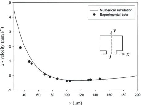
integrating the velocity field. (Marcos and Stocker 2006)...23 Figure 2-4. Velocity inside the cavity in the x - direction, as a function of the transverse position y (dashed line in the inset) for Uc = 363 [tm s- . Experiments (circles) are compared with numerical results (solid line). (Marcos and Stocker 2006). ... 23

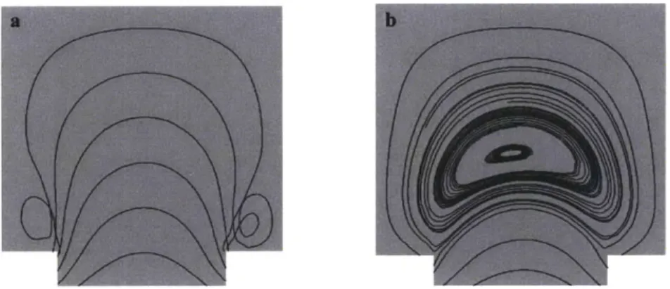
Figure 2-5. Numerical streamlines for UF = 21.4 [tm s1 and two different depths: (a) H =

70 jim; (b) H = 90 jm. All other dimensions are as in Fig. 3. Crossing streamlines visible

in panel (a) reflect small three-dimensional effects. ... 24 Figure 2-6. Two configurations in which no vortex formed, as shown by the trajectories of 2-pm beads: (a) a= 1, g = a = 200 jm; (b) a= 2, g = a/2 = 200 jm. For both cases, H =

130 gm and UF = 21.4 mm s-1. The scale is the same in the two panels. ... 24

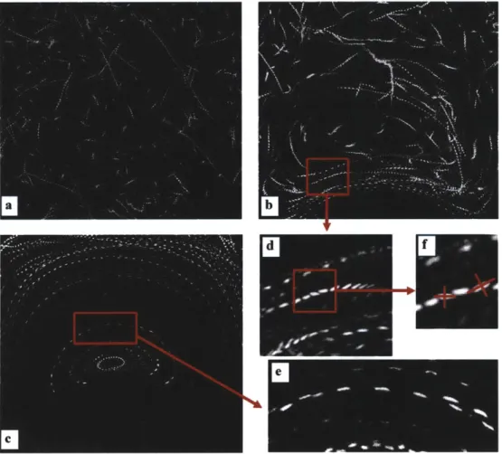
Figure 2-7. Trajectories of the bacteria P. haloplanktis in vortices of different strength: (a) No flow; (b) Uc = 36.3 ptm s-1 (c) Uc = 363 jim s-'. The field of view is shown in Fig. 1;

(d) and (e) are magnified views of selected trajectories, showing the instantaneous

orientations of individual bacteria; (f) A bacterium's orientation is further magnified to highlight misalignment with the direction of travel... 25

Figure 2-8. Trajectories of the alga D. tertiolecta swimming in the cavity: (a) No flow; (b)

Uc = 363 jim s~1. The field of view is shown in Fig. 2-1. The black spot inside each alga is a result of phase contrast m icroscopy. ... 26

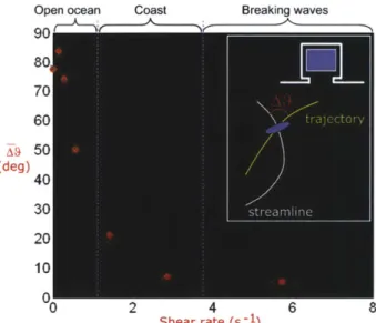
Figure 2-9. The average streamline crossing angle of P. haloplanktis swimming in a microvortex under various shear rates. The size of the analysis region (blue box, upper inset) is chosen arbitrarily within the field of view. The shear rate is averaged over the

region of analysis. Red filled circles are the data obtained from the region of analysis. Green and yellow crosses are the data obtained by increasing and decreasing the region of analysis by 20%. The lower inset shows the definition of streamline crossing angle AO .... 28 Figure 3-1. Schematic of a straight rod in a simple shear flow...30 Figure 3-2. Schematic of helix in a body fixed frame OXYZ...32 Figure 3-3. Euler angles describing the body orientation. The arrow represents the major axis of the b ody ... 33

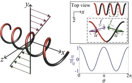
Figure 3-4. Schematic of a right-handed helix in simple shear flow. Red shading and black shading show the top and bottom halves of the helix. Upper inset: The net force acting on one pitch of the helix is along -z. Lower inset: Predicted normalized drift velocity v/vo versus helix orientation 9. 9 is the angle between a helix in the x-y plane and the flow, and

vo is the drift velocity of a helix aligned with the flow (9 = 0, y = iC/2). (Marcos et al.

2 0 0 9 ). ... 3 5

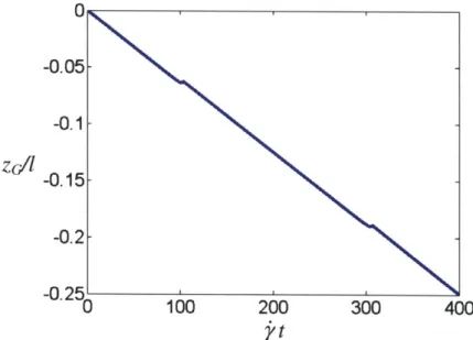
Figure 3-5. Predicted lateral drift of a right-handed helix in simple shear flow in the

absence of Brownian motion. The number of full turns is n = 25, pitch angle a= 450, total

contour length I = 14.1 gm, and we assumed

4i/{,l

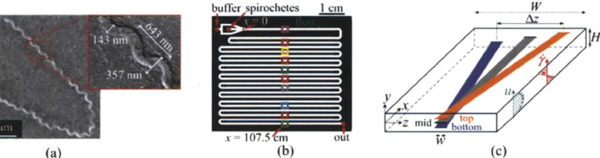
Figure 3-6. (a) Scanning electron micrograph (SEM) of L. biflexa flaB mutant, with typical dimensions (inset). The bent configuration is a result of SEM preparation and live organisms are nearly always straight. (b) Microchannel design with separate inlets for spirochetes and buffer. The color-coded squares refer to the locations of data collection (Fig. 3-7b). (c) Schematic of the separation process (for right-handed helices) in the microchannel (W = 1 mm, H = 90 pm, w ~ 100 pm). The lateral drift direction depends on

the sign of the shear ?, resulting in divergence of top and bottom streams. (Marcos et al.

2 0 0 9 ). ... 3 7

Figure 3-7. Observed spirochete distributions across the channel width for (a) x = 2 cm and (c) x = 107.5 cm. Orange, black, and blue correspond to the top, mid, and bottom

depths. The midpoint of each rectangle corresponds to the mean position ( -) of the

distribution, while the half-width is 2 standard deviations (2o). b) Probability distribution function, obtained from fifty images at each location, for various distances x along the channel. Over 10,000 spirochetes were imaged for each location x, y. The broadening of the population distribution is accounted for by the finite depth of focus of the imaging system, combined with variation of shear (hence, drift) with depth. (Marcos et al. 2009). 38 Figure 3-8. The standard deviation a-of the spirochete distribution versus distance x in the microchannel. Circles are experimental data, color-coded according to depth as in Fig. 3-6c. Solid and dashed lines refer to values calculated with a depth of focus S= 10 pim and 14 gm, respectively, while green and red lines correspond to y = H14 (or, equivalently, y =

Figure 3-9. Experimental quantification of spirochete distribution: a) Average lateral position at top, mid, and bottom depths, and b) separation between top and bottom populations, as a function of distance x along the channel. c) Hypothetical separation efficiency. In a), b), and c), full circles are data from spirochetes, lines are linear fits, and empty squares are control data from spherical beads. (Marcos et al. 2009). ... 40

Figure 3-10. The effect of the polar angle Von the drift velocity v. vo is the drift velocity of a helix aligned with the flow (0= 0; y= n/2). (Marcos et al. 2009)...41 Figure 3-11. Size limit for separation of isometric helices of length L and equivalent aspect ratio r = 70. Dashed contours show constant Re (spaced by a factor of 10) and the thick

contour is Re = 0.1. Solid contours show constant Pe. The gray scale shows T / vo, where vo

is the drift velocity of a helix aligned with the flow. The smallest helices which can be separated for a given shear rate, determined by v/v0= 0.66 (Pe = 50, marked by circle on

inset) and Re < 0.1, have L ~ 20 (square), 80 (circle), and 400 nm (diamond) for k= 108,

106, and 104 s1, respectively. Full symbols mark the parameter regimes of our experiments:

Re = 0.03 (triangle) and Re = 5 (hexagon). Inset: v/vovs Pe. (Marcos et al. 2009)...43

Figure 4-1. Schematic of a bacterium in a simple shear flow...45 Figure 4-2. Sketch showing the center of the helix (H) and the center of the sphere (S), which are separated by a distance Ar in 3D space. p is a general point on the helix...46 Figure 4-3. a) The chirality-induced lateral drift force on a right-handed helical flagellum and the drag on the cell head lead to a reorienting torque on a bacterium. b) This chiral torque causes a swimming bacterium to preferentially point away from the x direction and thus to experience a net drift velocity V that is of the same order as the swimming velocity

U ... 4 9

Figure 4-4. Net drift velocity (V) of a population of swimming bacteria (black solid line), swimming ellipsoids (blue dashed line), and non-swimming bacteria (red dotted line) in a simple shear flow. The drift velocities of the three populations were normalized with the swimming speed of bacteria (U = 50 gm/s). The bacteria were modeled by assuming a 1

gm radius spherical head and a left-handed helical flagellum with 4 turns, pitch angle of 410 , and axial length of 10 gim, corresponding to the flagellar bundle of E. coli. For swimming bacteria, the angular rotation rate of the flagellum relative to the cell body 0)el =

12 7 H z ... 5 0

Figure 4-5. Effects of cell swimming speed on the net drift velocity (normalized with average swimming speed) under various shear rates. The model assumes a 0.2 gm radius spherical head and a left-handed helical flagellum with 3 turns, pitch angle of 370, and axial length of 6 pim, corresponding to the flagellar bundle B. subtilis...51 Figure 4-6. Effect of head size on the net drift velocity, normalized with the swimming speed U, as a function of the shear rate. The model assumes a left-handed helical flagellum

with 3 turns, pitch angle of 370, and axial length of 6 gm, corresponding to the flagellar bundle of B. subtilis. In all cases, U = 50 jm/s... 52

Figure 4-7. The effect of tumbles on the drift velocity. The net drift velocity (V) of a population of smooth- swimming bacteria (black) and run-and-tumble bacteria (blue). Effects of Brownian rotation are included in the model. The bacteria were modeled by assuming a 0.4 gm radius spherical head and a left-handed helical flagellum with 3 turns, pitch angle of 370, and axial length of 6 jm, corresponding to the flagellar bundle of B.

subtilis. The angular rotation rate of the flagellum relative to the cell body arel = 250 Hz,

giving swimming speed U = 50 pim/s. The run-and-tumble swimmer had an average

change direction of 680 and a standard deviation of 39' with mean run time r= 1 s...54 Figure 4-8. (a) Schematic of the chiral reorientation process at a quarter depth in the channel, i.e. y = -H/4, for a left-handed flagellum. The microchannel had width W = 1 mm, height H = 90 pm. (b) Microchannel design showing inlet and outlet. Note that only one

inlet was used in this experiment. The square refers to the location of data collection and was located 110 cm downstream of the inlet. (c) Two sample trajectories of B. subtilis bacteria in a shear flow, imaged at y = -H14. The center of the colored circles corresponds

to the locations obtained by the image processing routine. ... 56

Figure 4-9. Net drift velocity of B. subtilis 014139 under various shear rates at y = -H/4,

normalized by the mean average swimming speed U = 55 jim s-1. Each set of colored

squares indicates a separate batch of bacteria. Six replicates were performed. Solid lines refer to the theoretical prediction assuming a left-handed helical flagellum with 3 turns, pitch angle of 370, and axial length of 6 jm, and a spherical head of radius 0.4 jm (black line) and 0.8 jm (blue line)... 56

Figure 4-10. Net drift velocity of B. subtilis 014139 under various shear rates at y = H/4

and y = -H/4, normalized by the mean average swimming speed U= 55 jm s-. Since the

shear rates between the top and bottom layer are opposite in sign, we present the absolute values of the shear rate. Two separate sets of experiments (light and dark colors) were conducted at y = H/4 (red) and y = -H/4 (green). For each case, two replicates were

performed. The two experiments at y = -H/4 were performed in addition to the ones

show n in F ig . 4 -9 . ... 57

Figure 4-11. Swimming trajectory of B. subtilis 014139 in the absence of flow. Several trajectories show a helical pattern, visualized as a sinusoidal path when viewed from the to p ... 5 8

Figure 4-12. Schematic of a generalized swimmers, based on three spheres to model an elongated cell head and on an off-axis flagellar bundle, which induces wiggling. Angle AA denotes the contact point between cell body and the flagellar bundle. Lower inset: Angles BB and CC are the polar and azimuthal angles of the flagellar bundle (thick green arrow) relative to the cell body (body fixed frame OXYZ)... 59

Figure 4-13. Wiggling in the trajectory of a swimming bacterium in the absence of flow. The ellipsoid represents the cell head of the bacterium. The flagellar bundle is offset relative to the cell body axis by 180. The red point shows the initial position of the bacterium at the start of the simulation and the solid line shows that trajectory of the center of the middle sphere. The inset shows the trajectory as viewed from the top. The model assumes a left-handed helical flagellum with 3 turns, pitch angle of 370, and axial length of

6 ptm, corresponding to B. subtilis flagellar bundle and a cell head made of three spherical

heads of radius 0.5 gm. The three angles determining the flagella bundle offset are AA =

CC = 0 and BB = 180. Brownian motion was neglected in this simulation...62

Figure 4-14. Effects of elongation and wiggle on the net drift velocity. The model assumes a left-handed helical flagellum with 3 turns, pitch angle of 370, and axial length of 6 gm. The black line shows the theoretical prediction that agrees well with the experimental data (see Fig. 4-9). The 3-sphere model was calculated using 3 identical spheres of radius 0.5 gm (cyan). The three angles determining the flagellar bundle offset are AA = CC = 0 and

B B = 50 (red )...6 3

Figure 4-15. Time evolution of the mean swimming speed of a bacterial population after exposure to a shear rate of 500 s-1 for 9 minutes. Colors refer to Pseudoalteromonas

haloplanktis (blue), Bacillus subtilis (black), Escherichia coli (green), and Pseudomonas aeruginosa (red). Solid lines refer to the values before shear exposure. ... 64

List of Tables

Table 2-1. The influence of advection on P. haloplanktis and D. tertiolecta in vortices of various strengths. An equivalent dissipation rate E is calculated based on UC. Symbols indicate the importance of advection by the vortex over motility as inferred from

trajectories, from '++' (advection dominates) to '- -' (motility dominates). ... 27

Table 3-1. Comparison of VI/vo between 2D and 3D models. vo is the drift velocity of a helix aligned with the flow (6= 0, y= ir/2). (Marcos et al. 2009)...42

Chapter 1

Introduction

Microorganisms are ubiquitous in the environment. Despite their tiny size, their combined biomass is enormous. The functions performed by microorganisms play a critical role in nearly every environment (Weeks and Alcamo 2008). In soil, almost every chemical transformation involves active contributions from microorganisms. In particular, microbes play a fundamental role in soil fertilization by mediating the cycle of nutrients like carbon and nitrogen, which are crucial for plant growth (Wheelis 2008). In the ocean, microorganisms are important not only because they form the base of the marine food web, but also because they drive biogeochemical cycles, including carbon, nitrogen, sulfur and iron (Willey et al. 2008). Their activities can affect local meteorological patterns and potentially influence changes in global climate. Other microorganisms are pathogenic and negatively affect humans, such as Salmonella, which contaminates water supply systems,

or Helicobacter, which gives ulcers, or Pseudomonas, implicated in cystic fibrosis (Willey

et al. 2008). Many species of bacteria form biofilms, surface-attached microbial colonies encased in a polymeric matrix, which arise on nearly every surface in a wide range of environments and cause huge economics losses resulting from equipment damage, product contamination, and energy dissipation (Hui 2006).

Microbes nearly always inhabit a dynamic environment and are exposed to a range of flow conditions: creeping flow in soil, highly sheared flow in bodily conduits, and turbulent flow in rivers, streams, lakes, and oceans, as well as in anthropogenic habitats such as bioreactors, heat exchangers, and water supply systems. The presence of flow not only affects how microorganisms are transported and dispersed at the macroscale, but also their ability to interact with their local habitat through motility and chemotaxis (the ability to sense and follow chemical gradients), in particular their foraging. For example, the development of biofilms in pipes and channels depends on the flow conditions (primarily shear) at the surface on which the biofilm lives. For free-living (or 'planktonic') microorganisms, motility has evolved as an important trait in escaping predators, finding refuges and exploring new environments. Most importantly, microbes swim to take advantage of spatially heterogeneous nutrient sources, which are often patchy down to scales of micrometers (Azam 1998; Blackburn et al. 1998; Seymour et al. 2000; Stocker et al. 2008).

Many microorganisms use one or more appendages to swim. At the length scales of microorganisms, the inertia of both the cell and the fluid is unimportant and viscous effects dominate: the Reynolds number is very low. The Reynolds number is a dimensionless quantity defined as Re = pUL/u, where p and u are the density and dynamic viscosity of the fluid, respectively, and U and L are the velocity and length scales of the flow, respectively. In water (p ~ 1000 kg m-3, U 10-3 kg m- s-1), a swimming bacterium such as

10-10-4. A human spermatozoon with U ~ 200 ptm s-land L ~ 50 jim moves with Re ~ 10-2

(Brennen and Winet 1977; Lauga and Powers 2009). Given the smallness of the inertial effects, it is appropriate to study bacterial fluid dynamics in the limit of zero Reynolds number, for which the governing equations of fluid motion are the Stokes equations

-Vp+pV 2u=0, V -u=0, (1.1)

where u and p are the velocity and pressure of the fluid.

Since Eq. (1.1) is linear, hydrodynamic forces are linearly related to the flow velocities. In addition to this linearity, one other important property in Stokes flow is drag anisotropy, a crucial ingredient for biological locomotion at zero Reynolds number (Hancock 1953; Lauga and Powers 2009). For example, at low Reynolds number a rod has more resistance when moving perpendicular rather than parallel to the flow. Therefore, to obtain the same velocity, moving the rod in the perpendicular direction requires more applied force than moving it in the parallel direction.

The linear and time-independent nature of the Stokes equations lead to kinematic reversibility (Happel and Brenner 1965), where the distance travelled by a swimmer does not depend on the rate of the motion, but only on the geometrical motion itself. Furthermore, if the sequence of motions displayed by a swimmer in a time-periodic fashion is identical when viewed after a time-reversal transformation, then the swimmer cannot move on average. This property is also known as the 'scallop theorem', where reciprocal motion, such as a clapping scallop that opens and closes its shell periodically, generates no net motion (Purcell 1977; Lauga and Powers 2009). Therefore, in order to swim in the low Reynolds number regime, microorganisms must adopt non-reciprocal body motions. Well-known examples include sperm cells, which swim by sending traveling waves of bending down flexible flagella (Bray 2001), and bacteria, which swim

by rotating helical flagella (Berg 2004). The detailed morphology of bacterial flagella

varies from one species to another (Fujii et al. 2008). For example, Escherichia coli forms a left-handed helical flagellar bundle with 4 turns, a pitch angle of 410, and an axial length of 10 gm. Bacillus subtilis forms a 3-turn left-handed helical bundle, with a pitch angle of 370 and an axial length of 6 gm (Fujii et al. 2008).

Wild-type swimming bacteria, such as E. coli and B. subtilis, typically display a so-called 'run-and-tumble' swimming behaviour (Berg 2004). During runs, the bacterium swims along a roughly straight path, and its flagellar filaments are bundled together tightly behind the cell. During a tumbling event, the flagella come out of the bundle, resulting in a random reorientation of the cell before the next run. In the absence of chemical gradients, a bacterium's trajectory has many characteristics of a random walk. In the presence of chemical gradients, bacteria are able to swim up/down the gradients (i.e. performing positive/negative chemotaxis) by biasing their random walk. When bacteria move towards a food source, they prolong the duration of runs in that direction (or, equivalently, tumble less often when going in the right direction). This allows them to head towards the food source, with a net drift velocity or 'chemotactic velocity'. The chemotactic velocity

typically ranges between 6-23% of the swimming speed, but can be as high as 35% (Ahmed et al. 2010b).

In addition to chemical gradients, the life of microorganisms is governed by flow. A naYve treatment would only consider flow as a source of advection, which transports bacteria along streamlines. However, fluid flow also involves velocity gradients (i.e. shear), which could significantly alter bacterial swimming trajectories. The shear intensity varies from one environment to another. For example, the shear rate can be as large as 1 s-1 in the open ocean (Lazier and Mann 1989) and in lakes (MacIntyre et al. 1999, 2002), ~ 4 s-1 in the coastal ocean (Kunze et al. 2006), ~ 20 s-1 in human's gastric tract (Kozu et al. 2010), and shear rates above 40 s-I are usually found in engineered water treatment systems (Crittenden et al. 2005).

At low Reynolds number shear flows, objects undergo periodic rotations known as Jeffery orbits (Jeffery 1922): a sphere rotates with constant angular velocity, whereas for an elongated body, the velocity depends on orientation. The more elongated a body, the longer its relative residence time when aligned with streamlines. Non-chiral objects, such as spheres and ellipsoids, follow streamlines in a low Reynolds number shear flow (Jeffery

1922). On the other hand, chiral objects, such as helices, drift across streamlines when

exposed to shear (Brenner 1964; Kim and Rae 1991; Makino and Doi 2005; Marcos et al.

2009). The interaction between the morphology of microbes and a shear flow is therefore

important in determining swimming trajectories, in particular the ability of bacteria to swim across streamlines.

Despite the ubiquitous presence of flow in the environment of microorganisms, very few studies have focused on the hydrodynamic interaction between flow and swimming in microbes. The existing studies are prevalently numerical. It was shown that bacteria can cluster around phytoplankton cells (Bowen et al. 1993; Luchsinger et al. 1999) and around sinking aggregates such as marine snow particles (Kiorboe and Jackson 2001). Meanwhile, solution of the stochastic evolution equations for a bacterial population (Bearon and Pedley 2000; Bearon 2003; Locsei and Pedley 2008) has shown that reorientation due to Jeffery orbits can render run-and-tumble chemotaxis ineffective at high shear rates (Locsei and Pedley 2008). However, in these studies, bacteria were simply modeled as either spheres (Bowen et al. 1993; Kiorboe and Jackson 2001) or ellipsoids (Luchsinger et al. 1999; Locsei and Pedley 2009), neglecting the detailed morphology of bacterial cells, and thus chirality.

A small number of studies have considered the effects of flow on microbial motility.

Among these are the discovery of rheotaxis in spermatozoa (Bretherton and Rothschild

1961) and gyrotaxis in biflagellated swimming algae (Kessler 1985). Rheotaxis refers to

the tendency of organisms to align with the direction of flow. The organism exhibits a positive/negative rheotaxis when its head points upstream/downstream, respectively. For example, in a horizontal Poiseuille flow, live spermatozoa have been observed to exhibit positive rheotaxis (Bretherton and Rothschild 1961). Rheotaxis can be either a hydrodynamic or a behavioral effect. Gyrotaxis is a process in which the preferred orientation of a bottom-heavy cell is determined by a balance between the viscous torque

and the gravitational torque. Due to gyrotaxis, in a downward cylindrical Poiseuille flow, uniformly suspended algae swim towards the axis of the tube, whereas they swim toward the periphery in an upward flow (Kessler 1985).

Other examples of the effect of flow on microbial motility concern phytoplankton and spermatozoa. Using a Taylor-Couette apparatus, it was found that the orientation of swimming dinoflagellates in a shear flow was significantly different from random, with a preferential alignment at an angle with the flow (Karp-Boss et al. 2000). This observation was rationalized as differences in drag forces on the body and flagella (Karp-Boss et al. 2000). Other studies found that fertilization success in the purple sea urchin depends on intensity of the shear (Mead and Denny 1995; Riffel and Zimmer 2007). Low shear rates improve fertilization through mixing enhancement and thus increasing the encounter rates between sperms and eggs. On the other hand, large shear rates overwhelm the sperm's ability to reach the egg. (Riffel and Zimmer 2007).

It has been known for some time that surfaces affect how nearby bacteria swim, giving rise to circular trajectories in horizontally unconfined environments, or the "swimming on the right" behavior in microchannels (Ramia et al. 1993; DiLuzio et al. 2005; Lauga et al.

2006). The circles result from the cell body and flagella rolling along the surface in

opposite directions, creating a torque that makes the cell swim in circular trajectories (Lauga et al. 2006). In the presence of shear, this behaviour changes drastically: E. coli were found to swim upstream in a microfluidic channel under shear flow (Hill et al. 2007). This ability to swim upstream could be crucial in colonizing urinary tracts, causing infection. These studies demonstrated that novel processes are uncovered and important new insight is gained by 'simply adding flow' to the microbial world.

Most techniques used to date do not allow direct observation of bacterial movement patterns in flow, due to the difficulty in setting up accurate and controllable flow fields while visualizing and quantifying the microorganisms' response. Here we propose that microfluidics enables one to work at the appropriate scales, both in terms of the manipulation of flow, as well as the direct visualization of how microorganisms are affected by flow.

Microfluidics has triggered important advances in a range of fields, from cellomics to chemical engineering, due to the opportunity to carefully control geometries, flows and chemical gradients, while observing the response of the system at the scale of micrometers (Whitesides et al. 2001; Marcos and Stocker 2006; Seymour et al. 2007). Yet, the application of microfluidics to understand fundamental interactions between flow and swimming microorganisms has been lagging. This thesis takes a first step in this direction

by exploiting microfluidics to study the effects of shear on bacteria.

This research began with the use of microfluidic technology to understand the response of microorganisms, such as bacteria and algae, to a highly simplified model turbulent environment. At the small scales of these organisms, turbulence is experienced simply as shear: understanding the interaction between shear and swimming is then a critical step towards gaining insight in how the ambient flow favors or hinders microorganisms in their

quest for food. Realizing that microbial morphology plays an important role, this thesis seeks to understand the hydrodynamic interaction between shear and shape in the bacterial world.

The goal of this thesis is to investigate the role of flow on the motility of bacteria, both experimentally and theoretically. The specific aims of this research were to:

1. Develop a mathematical model of a swimming bacterium in a shear flow.

2. Design and carry out experiments to study the effect of shear on bacterial motility.

3. Investigate whether bacteria display a behavioural response to hydrodynamic shear,

as evidence that they can sense hydrodynamic shear.

In chapter 2, we develop a new method to generate microscale vortices (akin to the smallest components of turbulence in the ocean) using a microfluidic setup, with accurate control and visualization of the flow. We discuss the effects of vortex strength on the swimming of marine bacteria and algae.

In chapter 3, we develop a mathematical model employing resistive force theory to study the hydrodynamic effect of shear on a rigid, non-swimming helix, relevant to the helical shape of bacterial flagella and some species of microorganisms, such as spirochetes and

Spirulina. An experimental verification of the theory by exposing the non-motile, helically

shaped bacteria Leptospira biflexaflaB mutant to shear in a microfluidic channel is given. We present the full model of bacteria swimming in a shear flow in chapter 4. We discuss the role of randomness in swimming and the effect of cell size on the cell's ability to swim across streamlines. A set of experiments is presented to verify the model by exposing the smooth swimming bacterium Bacillus subtilis 014139 to a microfluidic shear flow. Finally, to confirm whether the observations are the result of purely hydrodynamics effects, we present a separate experiment to probe the bacteria's ability to actively respond to shear.

Chapter 2

Bacteria swimming in microvortices

Eddies at the Kolmogorov scale (e.g. Yamazaki et al. 2002) are the smallest remnants of the turbulent cascade in the ocean, with time scales in the order of 1-100 s, depending on the intensity of turbulence (Karp-Boss et al. 1996). Kolmogorov eddies represent fluid motion at the scale most directly relevant to microbial dynamics, affecting nutrient redistribution by shear (Bowen et al. 1993; Luchsinger et al. 1999), encounter rates with predators and nutrient patches (Rothschild and Osborn 1988), and the ability of microorganisms to swim and chemotactically orient in the flow. Quantitative experimental information on microbial dynamics at these scales is still lacking. We propose to use microfluidics as a first step in understanding the response of microorganisms to microscale vortices. The generation of vortices at small Reynolds numbers has been investigated both experimentally and numerically (Higdon 1985; Shen and Floryan 1985). At the microscale, great attention has been devoted to flows that enhance mixing (e.g.: Liu et al. 2000; Stroock et al. 2002), but the time-scales do not reflect those relevant in the environment (e.g. Shelby et al. 2003). Yu et al. (2005) used side cavities to generate vortices in microchannels and mapped out the regime in which flow separation is to be expected. Here we apply a similar technique to generate stable microvortices on scales relevant to microbial dynamics in the aquatic environment, and show that we can obtain detailed information on the microorganisms' response.

2.1 Materials and procedures

2.1.1 Fabrication

Channels were fabricated using soft lithography (Whitesides et al. 2001, Seymour et al.

2007). Fabrication begins by creating a blueprint for the microchannels using

computer-aided design (CAD) software and printing it on transparency film with a high-resolution image setter to create a 'mask' (Fineline Imaging, Colorado Springs, CO). A silicon wafer is spin-coated with a layer of negative photoresist (SU8-2100, MicroChem, Newton, MA), the thickness of which corresponds to the final depth of the channels. With the mask laid on the coated wafer, the latter is exposed to UV light, polymerizing exposed regions of the photoresist. After dissolving the unpolymerized photoresist, the channel structure is left on the wafer (the 'master'). The soft polymer polydimethylsiloxane (PDMS, Sylgard 184; Dow Corning, Midland, MI) is prepared according to the manufacturer's instructions and poured on the master to cast PDMS channels. After curing the PDMS by baking for 12 h at

650C, the PDMS layer containing the channels is peeled off from the master, and holes for

inlets and outlets are punched with a gauge 16, sharpened luer tip. Finally, channels are bonded to a glass slide after treating both the PDMS layer and the glass slide with oxygen plasma for 1 min (HARRICK Plasma Cleaner/Sterilizer, Harrick Scientific, Ossing, NY).

2.1.2 Microchannel geometry

The channel has a rectangular cross section of width W and a rectangular side cavity of length a and width b (Fig. 1). The depth, H, is the same for the main channel and the cavity. Differently from Yu et al. (2005), we partially closed the area between the cavity and the main channel, leaving an opening of length g. In our basic configuration, L = 10 mm, a =

W = 200 gm, H = 130 jm, d = 25 jm, g = 120 pm, and the cavity aspect ratio a= a/(b+d)

= 1. We also considered two additional configurations, g = a = 200 jm and a = 2,

respectively. Y -a----| cavity

xbT

Figure 2-1. Geometry of the microchannel. Gravity is in the -z direction (into the plane). The cavity and the channel have the same depth, H. The dashed line shows the field of view where microorganisms are tracked. Mean velocity in the main channel is UF; characteristic velocity inside the cavity is Uc. (Marcos and Stocker

2006).

2.1.3 Experimental setup

The microchannel was set on the stage of a Nikon Eclipse TE2000-E inverted microscope (Nikon, Japan). PEEK tubing (0.762 mm ID, 1.59 mm OD, Upchurch Scientific, Oak Harbor, WA) was used to connect the inlet to a 10 mL syringe (BD Luer-Lok Tip) via a fitting (Part P-704-01, Upchurch Scientific, Oak Harbor, WA) and the outlet to a constant-depth reservoir, to avoid capillary and gravity effects (Fig. 2-2). A constant flow rate in the main channel was generated using a syringe pump (PHD 2000 Programmable, Harvard Apparatus, Holliston, MA). For the appropriate geometrical configuration, the shear stress of the main flow produced a vortex in the cavity of strength proportional to the mean velocity UF in the main channel.

condenser and

light source _{cavity tbn}

syig glass § ide PE7 ubn

syringe pump IA inlet outlet

- objective reservoir microscope stage

to CCD camera

Figure 2-2. Schematic of the experimental setup. The microchannel is set on the stage of an inverted microscope and flow is driven by a syringe pump. Microorganisms in the cavity are imaged with a CCD camera. (Marcos and Stocker 2006).

The flow field within the channel was visualized using 2-jm diameter beads (Polysciences, Warrington, PA). Phase contrast was used to image the beads and the microorganisms,

with long-working-distance 20x (NA = 0.45) and 40x (NA = 0.6) objectives. The depth of

field can be calculated following Meinhart et al. (2000): for 2-pm beads, we obtained 28 Rm (20x) and 19 gm (40x). Sequences of images ('movies') were captured with a 1600 x 1200 pixels, 14 bit, cooled CCD camera (pixel size 7.4 x 7.4 gm2; PCO 1600, Cooke, Romulus, MI) at 30 to 62 frames s-1 and processed using IPLab software (Scanalytics, Fairfax, VA). In the images, beads or microorganisms appear as bright regions on a darker background. Images of the trajectories were obtained by assigning to each pixel the maximum light intensity recorded in that pixel over the duration of the movie (3D Time

Stacked View command in IPLab).

2.1.4 Numerical modeling

For preliminary screening of a range of design configurations, as well as for accurate characterization of the flow field, we carried out a computational fluid dynamics simulation of the cavity flow. We used the finite-element code Comsol Multiphysics (Burlington, MA) to solve the steady-state Navier-Stokes equations in three-dimensional space. The model geometry was that described above, except for L = 1 mm to save computational time (we verified that the flow field in the cavity is the same as for L = 10

mm). The boundary conditions were no-slip on all solid boundaries, uniform velocity at the inflow and zero pressure at the outflow. We adopted a multigrid solver using between

13,000 and 22,000 elements, each at most 30 jim in size.

2.1.5 Microorganisms

The marine bacterium Pseudoalteromonas haloplanktis (2 [tm length) was grown to exponential phase in 1% Tryptic Soy Broth (TSB) at room temperature, before being diluted 1:10 in Artificial Seawater. Experiments were performed 72 hours later. The motile marine alga Dunaliella tertiolecta (5 jim diameter) was grown to exponential phase in f/2 medium.

2.2 Assessment and discussion

Using the setup described above we were able to generate a stable and reproducible vortex in a cavity of aspect ratio a = 1 (Fig. 2-3a). The numerical streamlines (Fig. 3b) closely match the experimental trajectories, as expected for a steady flow. Good agreement is further demonstrated by comparing the velocity measured experimentally at different locations in the cavity with its numerical counterpart (Fig. 2-4). We can therefore use the numerical model to investigate the vortex in more detail. For our geometry, the maximum velocity in the cavity is Uc = 1.7% UF for a main-channel Reynolds number Re = UFW/v <

6 (where v is the kinematic viscosity), corresponding to UF < 30 mm s1. In contrast to higher Reynolds number designs (e.g. Shelby et al. 2003), generation of the vortex does not rely on inertial effects. While the flow inside the cavity is in principle three dimensional, the vertical velocity (along z) is always much smaller than the horizontal velocity at the mid-depth plane, where all observations are made.

Figure 2-3. The flow in a cavity of aspect ratio a= 1, main flow speed UF = 21.4 mm s-1. The characteristic velocity in the cavity is Uc = 363 [tm s-1. Lengths of the cavity and the opening are a = 200 gm and g = 120 gm, respectively. Flow is from left to right. The cavity Reynolds number (Uc a/v) is 0.07. (a) Trajectories of 2 pm beads. The solid white line shows the outline of the channel. (b) Numerical streamlines at the mid-depth plane (z = H/2 = 65 gm). Imperfections in the streamlines result from small numerical errors in

integrating the velocity field. (Marcos and Stocker 2006).

5 - Numerical simulation 4 0 Experimental data 7c~ 3 - _ly o L 0 X ii 0 0-40 60 80 100 120 140 160 180 200 y (pm)

Figure 2-4. Velocity inside the cavity in the x - direction, as a function of the transverse position y (dashed line in the inset) for Uc = 363 [tm s-1. Experiments (circles) are compared with numerical results (solid line).

(Marcos and Stocker 2006).

2.2.2

Effects of the cavity geometry

Because of the fabrication processes involved in soft lithography, shallower channels are easier and faster to fabricate and, in general, the depth H is limited to about 1 mm. On the other hand, a minimum depth is required to generate a vortex. For our basic configuration, a vortex starts to form for H = 80 pm (not shown) and is fully developed for H 90 pm (= 0.45 a; Fig 5b).

Figure 2-5. Numerical streamlines for UF = 21.4 [tm s-1 and two different depths: (a) H = 70 gm; (b) H = 90 jm. All other dimensions are as in Fig. 3. Crossing streamlines visible in panel (a) reflect small three-dimensional effects.

It is interesting to note that this minimum depth changes with the cavity opening length g, not considered in previous studies. It has been shown that a two-dimensional flow (i.e., H

-> oo) in a fully open cavity (g = a) generates a vortex for aspect ratios a< 2 (Higdon 1985;

Shen and Floryan 1985; Yu et al. 2005). In three-dimensional low Re nolds number flow (Re* = Re Ac < 10), however, a vortex is expected only for Ac = (H/a) > 0.327, predicting

a minimum depth H = 0.57a for Re < 30.6 (Yu et al. 2005). We confirmed this prediction

numerically by testing the case g = a for H = 90 pm (Ac = 0.203, Re*= 1.25), finding

indeed no vortex. Partially closing the cavity opening g, on the other hand, introduces an additional degree of freedom, which we discovered reduces the minimum depth required for vortex formation. This can be seen by comparing Fig. 2-3 (g = 120 pm; a vortex forms) with Fig. 2-6a (g = 200 pm; no vortex), both obtained with H = 130 gm. Finally, no vortex

formed for a= 2, even for g = a/2 (Fig. 2-6b).

a b

Figure 2-6. Two configurations in which no vortex formed, as shown by the trajectories of 2-jm beads: (a) a

= 1, g = a = 200 gm; (b) a= 2, g = a/2 = 200 jm. For both cases, H = 130 pm and UF = 21.4 mm s~. The scale is the same in the two panels.

2.2.3 Trajectories and orientation of swimming microorganisms

Our aim in designing the cavity flow was to obtain a controlled, well-characterized flow field to study the response of microorganisms. In the previous sections, we have analyzed the formation of the vortex numerically and experimentally. Here we show that this setup also allows accurate visualization and quantification of the trajectories and instantaneous orientation of microorganisms swimming in the vortex, by applying it to the marine bacterium P. haloplanktis and the marine alga D. tertiolecta.

In order to have only motile organisms inside the cavity, we pre-filled the channel with fluid, injected the microorganisms, then stopped the flow: this procedure allowed some motile cells to spontaneously enter the cavity, at which point the flow was turned on again. Trajectories were imaged in the field of view shown in Fig. 2-1 (dashed line) at mid-depth (z = H12). A 40x objective was used for the bacteria and a 20x objective for the algae. No

effect of the microscope light on the microorganisms was observed.

Figure 2-7. Trajectories of the bacteria P. haloplanktis in vortices of different strength: (a) No flow; (b) Uc =

36.3 pim s1; (c) Uc = 363 tm s-1. The field of view is shown in Fig. 1; (d) and (e) are magnified views of selected trajectories, showing the instantaneous orientations of individual bacteria; (f) A bacterium's orientation is further magnified to highlight misalignment with the direction of travel.

In the absence of flow (Fig. 2-7a), P. haloplanktis swims in a random fashion, exhibiting a combination of long, straight runs, reversals and changes of direction, with a mean speed

of 55 gm s-1 and a maximum of 280 gm s-1. When the flow velocity in the vortex is considerably larger than the swimming speed (Fig. 2-7c), advection by the flow overwhelms motility and trajectories tend to streamlines. The elongated shape of P.

haloplanktis, characteristic of many species of bacteria, also allows detection of its

orientation in the flow field. In a strong vortex, bacteria not only follow streamlines, but they are aligned with them as a result of the shear in the vortex (Fig. 2-7e), except for the corner regions in the cavity, which the vortex does not reach (e.g. the top corners in Fig. 2-7c). The most interesting case is that of a vortex of intermediate strength (Fig. 2-7b), where bacteria can partially 'fight the flow': several trajectories cross streamlines and, even for those that do not, the shear is not strong enough to always align bacteria with the flow direction (Figs. 2-7d and 2-7f).

We further applied the microfluidic setup to the motile alga D. tertiolecta (Fig. 2-8), which swims up to 375 gm s-1 using two flagella. Its large size (5 [m) makes it easy to capture using video-microscopy, but its instantaneous orientation is more difficult to quantify due td its nearly symmetrical shape. Many species of phytoplankton in the ocean are known to use motility for phototaxis or chemotaxis, resulting in migration and clustering in preferential regions of the water column (Sjoblad et al. 1978; Eggersdorfer and Hader

1991). Phytoplankton motility is altered by small scale vortices, and the proposed setup

can help to quantify these changes (Fig. 2-8b).

a b

Figure 2-8. Trajectories of the alga D. tertiolecta swimming in the cavity: (a) No flow; (b) Uc = 363 pm s- .

The field of view is shown in Fig. 2-1. The black spot inside each alga is a result of phase contrast microscopy.

A preliminary quantification of the role of advection on motility can be obtained by visual

inspection of the trajectories and is summarized in Table 2-1. Motility of P. haloplanktis is not significantly affected for Uc < 36 ptm s-1, while advection dominates for Uc > 182 [Im

s-1. D. tertiolecta, on the other hand, can swim faster and exhibits higher thresholds (182 -363 [tm s-1) before being passively advected by the flow. In the ocean, turbulent dissipation

rates E range from 10-2 to 10- cm S-3 _{(Lazier and Mann 1989), corresponding to} Kolmogorov velocity scales of 1000 to 178 [tm s~1 (Yamazaki et al. 2002), respectively. While the main purpose of this calculation is to demonstrate the viability of the

...

experimental setup and not to provide a thorough quantitative analysis of the data, Table

2-1 suggests that bacteria would be mostly advected and aligned in a turbulent flow, while

motile algae can overcome mild turbulence levels.

Table 2-1. The influence of advection on P. haloplanktis and D. tertiolecta in vortices of various strengths. An equivalent dissipation rate E is calculated based on UC. Symbols indicate the importance of advection by the vortex over motility as inferred from trajectories, from '++' (advection dominates) to - (motility

dominates). UC P. haloplanktis D. tertiolecta ([m s- ) (cm2 _{S-3) (bacterium)} (alga) 9 6.8x10" -- --18 1.1 x 10-9 -- --36 1.7 x 108 - --91 6.8 x 10-7 + -182 1.1 x 105 + + + 363 1.7 x 104 _{+ +} +

Shear flows are known to affect the orientation of elongated bodies. Rigid spheroids undergo periodic rotation depending on their elongation (Jeffery 1922). In the case of swimming bacteria, orientation is governed by motility in addition to shear, and no theoretical prediction is available. We quantified the effects of shear on the ability of P.

haloplanktis to control its trajectory by determining the streamline-crossing angle AO

between a bacterium's trajectory and the local streamline (Fig. 2-9, inset). This angle is between 00 and 1800. When the bacteria are good swimmers or when the flow is weak, we expect the bacteria to swim randomly without following streamlines and thus the average

AO would be 900. On the other hand, when the bacteria are slow swimmers or when the

flow is strong, we expect the bacteria to follow the streamlines of the flow and thus small values of AO . Under weak flows, P. haloplanktis shows a random swimming pattern resulting in an average streamline-crossing angle close to 900. As the shear rate increases,

P. haloplanktis becomes more aligned with flow and thus AO decreases.

This result suggests that motile bacteria could stop swimming under highly turbulent conditions where swimming becomes energetically inefficient, as swimming consumes energy but no longer allows bacteria to move across streamlines into nutrient-rich environments. To ascertain this hypothesis, we plan to conduct experiments of bacterial active response to shear. Such experiments will be conducted in a parabolic flow field, since the flow field in the microvortex described above is complex and difficult to characterize.

A 50 (deg) 40 30 20 10 00 2 4 6 8 Shear rate (s-1)

Figure 2-9. The average streamline crossing angle of P. haloplanktis swimming in a microvortex under various shear rates. The size of the analysis region (blue box, upper inset) is chosen arbitrarily within the field of view. The shear rate is averaged over the region of analysis. Red filled circles are the data obtained from the region of analysis. Green and yellow crosses are the data obtained by increasing and decreasing the region of analysis by 20%. The lower inset shows the definition of streamline crossing angle AO.

2.3 Summary

We presented a microfluidic setup to generate vortices on scales relevant to microbial dynamics, while at the same time tracking responses of individual swimming microorganisms. We found that the formation of a vortex in the side cavity is dependent on the depth to width ratio (H/a) of the cavity, as well as the length of the opening (g) to the main channel.

We illustrated the ability of the setup to yield quantitative single-cell information on the behavior of microbes exposed to a recirculating shear flow. Steady flow in the cavity is only an approximation of Kolmogorov-scale eddies in the ocean, which are three-dimensional and unsteady (Karp-Boss et al. 1996), with time scales in the order of 1-100 s. While it would be possible to incorporate unsteadiness by modulating the flow in the microchannel over time using a programmable syringe pump, we believe the current setup in itself offers valuable insight on the fundamental interaction between microorganisms and their fluid dynamical environment (in particular the mean shear) at scales relevant to microbial dynamics, at least over times shorter than the Kolmogorov time-scale.

We envisage that microfluidic methods such as the one presented here will provide novel insight into the bounds that ambient flow imposes on the motility of microorganisms and on the behavioral strategies and dynamics of motile microbes living in a turbulent ocean. They will in turn impact our understanding of the role of microorganisms in the biogeochemistry of aquatic environments.

...

.... ... .... ... .. ... ...