Publisher’s version / Version de l'éditeur:
Vous avez des questions? Nous pouvons vous aider. Pour communiquer directement avec un auteur, consultez la première page de la revue dans laquelle son article a été publié afin de trouver ses coordonnées. Si vous Questions? Contact the NRC Publications Archive team at
[email protected]. If you wish to email the authors directly, please see the first page of the publication for their contact information.
https://publications-cnrc.canada.ca/fra/droits
L’accès à ce site Web et l’utilisation de son contenu sont assujettis aux conditions présentées dans le site LISEZ CES CONDITIONS ATTENTIVEMENT AVANT D’UTILISER CE SITE WEB.
11th International Symposium on Transport Phenomena and Dynamics of
Rotating Machinery [Proceedings], 2006
READ THESE TERMS AND CONDITIONS CAREFULLY BEFORE USING THIS WEBSITE. https://nrc-publications.canada.ca/eng/copyright
NRC Publications Archive Record / Notice des Archives des publications du CNRC :
https://nrc-publications.canada.ca/eng/view/object/?id=8c85d1b4-37bd-4958-a8fb-646dac95da83
https://publications-cnrc.canada.ca/fra/voir/objet/?id=8c85d1b4-37bd-4958-a8fb-646dac95da83
NRC Publications Archive
Archives des publications du CNRC
This publication could be one of several versions: author’s original, accepted manuscript or the publisher’s version. / La version de cette publication peut être l’une des suivantes : la version prépublication de l’auteur, la version acceptée du manuscrit ou la version de l’éditeur.
Access and use of this website and the material on it are subject to the Terms and Conditions set forth at
A linear regression model for marine propeller optimization,
prototyping and design
Proceedings of ISROMAC 2006: The Eleventh International Symposium on Transport Phenomena and Dynamics of Rotating Machinery February 26 - March 2, 2006, Honolulu, Hawaii USA
ISROMAC2006-69
A LINEAR REGRESSION MODEL FOR MARINE PROPELLER OPTIMIZATION, PROTOTYPING
AND DESIGN
Pengfei Liu *
National Research Council Canada
Institute for Ocean Technology Box 12093, 1 Kerwin Place St. John's, NL Canada A1B 3T5
Email: [email protected] Phone: 1-(709) 772-4575 Fax: 1-(709) 772-2462 Hong Wang Department of Mathematics and Statistics Faculty of Science, Memorial University of Newfoundland St. John's, Newfoundland A1B 3X5 Justin Quinton Faculty of Engineering and Applied Science Memorial University of Newfoundland St. John's, Newfoundland A1B 3X5 Brian Veitch Faculty of Engineering and Applied Science Memorial University of Newfoundland St. John's, Newfoundland A1B 3X5 ABSTRACT
A multiple-variable linear regression direct solution model and a statistical model were developed for marine propeller design, optimization and prototype. Computing implementation for the direct solution model was made to create an integrated tool for the marine propeller development process. An error analysis for a simple case with only 4 independent variables was performed. This direct solution model was constructed to provide two functionalities: generation of a set of linear regression coefficients to establish a multiple-variable polynomial equation and interpolation of the multiple-variable data set that are generated by the polynomial equations. An application case was given using a set of data from a marine nozzle propeller series both to cover interpolation to produce curves and linear regression coefficients for interpolation, for both the direct solution model and the statistical model that was computed under a commercial software package. Though much higher than the statistical model, interpolation by the direct solution model showed an error of less than one-tenth of a percent for a group of nozzle propellers. The highly computing-efficient direct solution method showed its capability as a general-purpose linear regression tool which can be applied widely for optimal product prototyping and design.
Keywords: Linear Regression, Optimal Prototyping and Design, Marine Propeller
INTRODUCTION
In the marine propeller design and optimization process, a set of performance curves are required for each candidate model propeller. These performance curves are namely the thrust coefficient Kt, torque coefficient Kq and propulsive efficiency
η, versus the advance coefficient J. For a special purpose
propeller series, typical performance curves are usually given for a propeller series via cavitation tunnel or tow tank tests, in terms of geometric parameters. These parameters are mainly the propeller disk expanded area ratio, EAR, with the same blade sectional shape, i.e., the same sectional profile, camber and maximum thickness distribution, the nominal pitch diameter ratio, p/D0.7R with the same pitch distribution along
the span of the blade, the number of blades, Z, each with the same blade planform contour. In propeller series model tests, a number of propeller models are manufactured to cover the possible range of geometric parameters for ship operation. A typical performance diagram is shown in Figure 1 as an example. The diagram is for a propeller with 4 blades (Z=4) and an expanded area ratio of 0.55 (EAR=0.55), It shows thrust curves versus the advance coefficient J for a range of pitch values from p/D0.7R =0.6 to 1.4, with an interval of
∆(p/D)=0.2..
For a comprehensive propeller series test, a number of propeller models must be manufactured and tested. If the tests are to cover a range of EAR from, say, 0.4 to 1.2 with an interval of 0.2, and the number of blades is from Z= 3 to 6, there will be 5 EAR values and 4 blade number values. Along with 5 pitch values from p/D0.7R = 0.6 to 1.4, a total of 100
propeller models must be manufactured. Increasing the intervals will reduce the number of propeller models required.
Thrust coefficient of a propeller of different pitch values -0.2 0.0 0.2 0.4 0.6 0.00 0.20 0.40 0.60 0.80 1.00 1.20 1.40 Advance coefficient J T h ru st co ef fi ci en t K t Kt 06Kt 12 Kt 08Kt 10 Kt 14
Figure 1. THRUST COEFFICIENT Kt OF A PROPELLER VERSUS ADVANCE COEFFICIENT J.
After the tests, a total of 20 propeller performance diagrams in the same form of Figure 1 can be plotted. The data obtained will be used to generate polynomial coefficients via linear regression and then establish a polynomial equation for propeller design and optimization with 3 independent variables, such as,
l k i l k R i L l K k I i t
EAR
p
D
J
C
K
0.7 , , 0 0 0)
/
(
)
(
∑
∑
∑
= = ==
(1)This work is to develop a numerical model to generate a set of cofficients for one or more independent variables in the form of Ci,k,l in equation (1) and use the coefficients and values of
independent variables to predict the hydrodynmic performance of an arbitrary canditate propeller within the series.
FORMULATION OF THE METHOD
To find a set of polynominal coefficients, for example with 4 independent variables, let the dependant variable:
)
,
,
,
(
x
1x
2x
3x
4f
y
=
, (2) be represented by:.
, , , 4 3 2 1 0 0 0 0 l k j i l k j i l l k k j j i iA
x
x
x
x
y
m m m m∑
∑
∑
∑
= = = ==
(3)For the simplicity of description, we set the values of the exponents im=1, jm=1, km=1 and lm=2. In practice, these values
are often taken as 6-8, considering both accuracy and conservation of computing resources. An expanded form of equation (3) becomes
.
2 4 1 3 1 2 1 1 2 , 1 , 1 , 1 1 4 0 3 0 2 0 1 1 , 0 , 0 , 0 0 4 0 3 0 2 0 1 0 , 0 , 0 , 0x
x
x
x
A
x
x
x
x
A
x
x
x
x
A
y
+
+
+
=
L
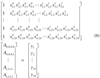
(4) Equation (4) has (im-0+1) (jm-0+1) (km-0+1) (km-0+1) = (1-0+1)×(1-0+1)×(1-0+1)×(2-0+1) = 24 terms. It may be written in a matrix form, which can be solved for the polynomial coefficients directly:[ ][ ] [ ]
X A =Y, (5) where [Y] is a vector storing 24 known values, which can beKt, Kq or η values of the propeller performance curves,
corresponding to the values of the independent variables raised to their respective powers and these values are stored in the square matrix [A].
Expanding equation 5, it gives:
⎥
⎥
⎥
⎥
⎥
⎥
⎦
⎤
⎢
⎢
⎢
⎢
⎢
⎢
⎣
⎡
=
⎥
⎥
⎥
⎥
⎥
⎥
⎦
⎤
⎢
⎢
⎢
⎢
⎢
⎢
⎣
⎡
⎥
⎥
⎥
⎥
⎥
⎥
⎥
⎦
⎤
⎢
⎢
⎢
⎢
⎢
⎢
⎢
⎣
⎡
24 23 2 1 2 , 1 , 1 , 1 1 , 1 , 1 , 1 1 , 0 , 0 , 0 0 , 0 , 0 , 0 2 24 , 4 1 24 , 3 1 24 , 2 1 24 , 1 0 24 , 4 0 24 , 3 0 24 , 2 0 24 , 1 2 23 , 4 1 23 , 3 1 23 , 2 1 23 , 1 0 23 , 4 0 23 , 3 0 23 , 2 0 23 , 1 2 2 , 4 1 2 , 3 1 2 , 2 1 2 , 1 0 2 , 4 0 2 , 3 0 2 , 2 0 2 , 1 2 1 , 4 1 1 , 3 1 1 , 2 1 1 , 1 0 1 , 4 0 1 , 3 0 1 , 2 0 1 , 11
1
1
1
y
y
y
y
A
A
A
A
x
x
x
x
x
x
x
x
x
x
x
x
x
x
x
x
x
x
x
x
x
x
x
x
x
x
x
x
x
x
x
x
M
M
L
L
M
M
M
M
L
L
(6)Once [A] is obtained, the polynomial equation is defined.
RESULTS AND DISCUSSION
Application case for the newly developed model
To test the method and its implementation, a set of propeller propulsive performance data was used [Yossifov et al. 1989]. Figure 2 shows a nozzle propeller in three different surface modeling approaches: hidden line, solid modeling and wire frame (Liu 2002 and Liu et al. 2002).
While in the figure only one combination of the propeller is shown, this propeller series has three different nozzles, N=1, 2 and 3, four nominal pitch values of (p/D)0.7R =1.0, 1.1, 1.2 and
1.3, and three EAR values of 0.5, 0.6 and 0.7. The dependent variable is either Kt, Kq or η and the four independent variables
are: N, ( p/D)0.7R, EAR and advance coefficient J.
Using the currently developed linear regression model, a set of polynomial coefficients can be obtained. These coefficients defined the polynomial equation which is,
) (J, N, p/D07 , EAR f
in a form of . ) / ( ) ( 0.7 , , , 0 0 0 0 i jkl l k R j i m l l m k k m j j m i i t N EAR p D J C K = ∑ ∑ ∑ ∑ = = = =
Figure 2. APPLICATION PROPELLER SERIES GEOMETRY.
The values of im, jm, km and lm are usually chosen at a small
value less than 10. For an 8-variable problem, if the value of the power is set at 8, the matrix size will be (9×9×9×9×9×9×9×9)2 =430467212 which needs about 1,380,000 GB of computing memory. For too large a matrix
size, an iterative solver should be used and the solver might need to be run under a parallel computing environment [Liu and Li 2002].
For this application case, for simplicity, we set im = 2, jm = 2,
km = 3 and lm= 6. The matrix size is then 2522. A total of 252
data points were prepared as in Table 1:
Table 1. INPUT DATA FORMAT AND LIST
N EAR PD J Kt 1 1 0.5 1.0 0.00 0.518087 2 1 0.5 1.0 0.14 0.433046 3 1 0.5 1.0 0.28 0.353132 . . . 252 3 0.7 1.3 1.14 -2.464862
The current model was used to generate a set of linear regression coefficients by solving for Ci,j,k,l to produce a polynomial . ) / ( ) ( 0.7 , , , 6 0 3 0 2 0 2 0 i jkl l k R j i l k j i t N EAR p D J C K = ∑ ∑ ∑ ∑ = = = = (8)
Plugging the values of these independent variables into equation (8) for the 252 data points, the Kt values are obtained
by the polynomial equation. Error estimation can then be done by comparing the Kt values from the polynomial equation with
those from Table 1 in terms of
%. 100 ) 0 ( ) ( ) ( % 1 2 1 × = − = J K J K J K E t t t (9)
The percent error for the 252 data points is plotted in Figure 3. %Error by current work
-3.00E-02 -1.00E-02 1.00E-02 3.00E-02 5.00E-02 7.00E-02 1 51 101 151 201 251 Data point ID P e rc e n t E rror fo r K t
Figure 3. ERROR IN PERCENT BY THE CURRENT NUMERICAL MODEL, DGSI.
It is shown in Figure 3 that the maximum percentage error is about 0.05%. This accuracy is sufficient for engineering design. A much higher accuracy may possibly be obtained when the value of the exponents is increased, though increased computing resources are also required. To generate these coefficients for a one-time execution, the implemented code
DGSI, took about a couple of minutes of CPU time on a 3.0 GHz PC.
Application Case for the Statistics Commercial Package SPlus and Comparison
Statistics model
The statistical method applied here is the traditional regression analysis based on multiple predictors that are identified as N,
EAR, (P/D)0.7R and J with a response variable Kt . First, we
establish a probabilistic model denoted by
. ) / ( ) ( 0.7 , , , 6 0 3 0 2 0 2 0 ε + ∑ ∑ ∑ ∑ = = = = = i jkl l k R j i l k j i t N EAR p D J C K (10)
where ε is the random factor having an approximately normal distribution with zero mean and constant variance. In this topic, this assumption is not critical because the data collected here only contain record errors.
Base on the observed data, we first form a 252×252 matrix for the factors Ni, (EAR)j , (P/D)k and Jl when i, j, k and l vary, so
that the regression formula (10) becomes , ε + ′ × =C A Kt (11)
where C is a 1×252 vector and A’ is the transpose of the 252×252 matrix.
The Least-square Method (LM) is employed to estimate C when K and A are observed. The basis of the LM method is to minimize the sum of squared errors:
.
)
(
_ _ 2∑
−
=
K
t originalK
t estimatedSSE
(12)Since there are 252 variables to be estimated in vector C with 252 observations, one will observe some singular terms in the process of minimization, which will yield zero estimates for those Ci,j,k,l coefficients. This is not a surprising result in this
kind of estimation process.
After the estimation procedure is carried out (here by S-Plus, an advanced statistical software package), the vector C will be estimated with (252 less the number of singulars) non-zero numerical values and the zero values will be assigned to those
Ci,j,k,l that are considered singular. After this process, a 1×252
vector C is generated. This can be viewed as a filtering procedure which will single out those Ni, (EAR), (P/D)k and Jl
terms that are not significant to the probabilistic model in equation (10).
Furthermore, more information in the regression analysis can be obtained such as the standard error, (t-value) and p-value (Pr((test statistic) >|t| )) for each Ci,j,k,l estimated. A sample
output of this information is listed Table 2:
Table 2. A SAMPLE OUTPUT FOR REGRESSION ANALYSIS Std. Error t value Pr(>|t|) 1 0.046340930 -16.613806360 1.154632e-14 2 0.267453190 1.421098450 1.681520e-01 3 1.079734330 0.470970110 6.419148e-01 . . . 26 0.981486080 -0.597363020 5.558597e-01 27 0.443841450 1.474089110 1.534547e-01 28 NA NA NA 29 0.156353330 7.597914470 7.765376e-08 30 0.851771110 -1.258532740 2.203047e-01 . . . 247 0.044432390 -0.704020400 4.881953e-01 248 NA NA NA 249 NA NA NA 250 NA NA NA 251 NA NA NA 252 NA NA NA
where the NA terms correspond to those zero (singular) valued Ci,j,k,l coefficients.
Since the critical p-value is provided in the output, the individual calculation formulas for standard error (and t value) become less important. One can find them in the text book. The use of the p-value for each term is to determine the significance of each Ci,j,k,l. estimated. For example, if the
p-value shown is 7.765376e-08, the corresponding C0,1,0,0 is
highly significant. To ensure maximum numerical accuracy, instead of abandoning all non-significant terms (such as the one shown with a p-value of 6.419148e-01, which is not statistically significant), we keep those very small but non-zero coefficients Ci,j,k,l so that those highly dependent
predictors remain in the polynomial in the deterministic component in equation (10).
Discussion of Regression Analysis Results:
Based on the propeller shaft torque (Kq) data set, which is
similar to the Kt data, we find that at 95% confidence level, the
difference (Error) between Kq and Kq_estimated) is estimated
within the confidence interval (1.529957e-05 2.228456e-05), which is close enough to zero. However, we could not conclude that the error is zero since the p-value for this test is 2.2e-16, which will reject the hypothesis that Kq-Kq_estimated=0
at almost any level of significance. Moreover, we have to admit that the Kq is over estimated by the regression model
defined in equation (10), even if it is by not that much.
Comparison between the Current Model (DGSI) and the Regression Model
Being given a data set like the propeller shaft torque (Kq) data
set, DGSI used a different approach to achieve the determination of the polynomial coefficients Ci,j,k,l. Based on
this single data set, we found that DGSI does a very good job to resolve the estimated Kq by those Ci,j,k,l coefficients resolved
by it.
It might be affected by the algorithm used in the DGSI procedure, but one has to notice that neither the estimated coefficients Ci,j,k,l nor the resolved Kq_estimated are consistent. In
other words, they are independent sets of estimates and evaluations.
One also needs to notice that at 95% confidence level, DGSI produces a wider confidence interval for the paired difference
(Kq-Kq_estimated) as (0.0001111199 0.0001467610) which is a
shift even more to the right. However, the mean of the differences is only 0.0001289405 which is again very close to zero. Not surprisingly, we will have to conclude that no evidence supports that the difference (Kq-Kq_estimated) is zero. In
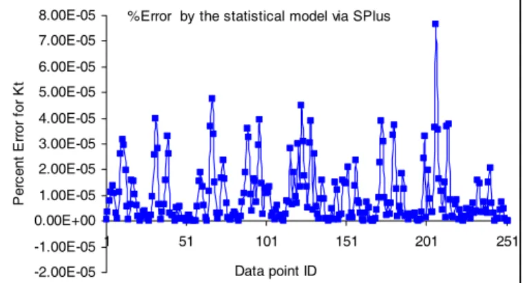
addition, we have to make clear that the above discussions in this section are based on a single set observations. A percentage error diagram for the statistical model via S-Plus is plotted and shown in Figure 4.
%Error by the statistical model via SPlus
-2.00E-05 -1.00E-05 0.00E+00 1.00E-05 2.00E-05 3.00E-05 4.00E-05 5.00E-05 6.00E-05 7.00E-05 8.00E-05 1 51 101 151 201 251 Data point ID Pe rc e n t Er ro r f o r Kt
Figure 4. PERCENT ERROR FOR THE ESTABLISHED STATISTICAL MODEL AND COMPUTED BY S-PLUS.
The direct solution method for linear regression coefficient developed in this work produced much larger percentage errors (0.005% versus 0.00007%) than the statistical model implemented and computed under S-Plus. A substantial accuracy improvement can be made if the direct solution model employed some kind of iteration process that requires more CPU time. However, the percentage error produced by the direct solution method without iteration is small enough for engineering design. Each run of the statistical model under S-Plus required about 4 hours (this includes the data format time on a P3 850MHz computer with 1GB RAM) of CPU time versus a couple minutes for the direct solution model implemented in DSGI (100:1). For the 4-variable problem, the saving of CPU by DSGI is not very significant. When the data points become larger and the power of the exponents is around 10, CPU time and memory could become prohibitive. Therefore, the current direct solution model is a good
alternative for engineering design applications, especially for a large number of independent variables and high exponential values.
CONCLUSION
A multiple-variable linear regression direct solution model and a statistical model were developed for marine propeller design, optimization and prototyping. Computing implementation for the direct solution model was made to create an integrated tool for the marine propeller development process. The direct solution model, without an iteration process, has a much larger error in percentage (0.005% versus 0.00007%) but is small enough for engineering design and computations. The statistical model via a commercial software package has a smaller percentage error with a requirement of much longer CPU time (100:1). For a linear regression task with a large number of independent variables and high order of exponent, the current developed model could be a better alternative.
ACKNOWLEDGMENTS
The authors would like to thank National Research Council Canada, Natural Sciences and Engineering Research Council Canada and Transport Canada for their support. We are also grateful to Mr. Mohammed Fakhrul Islam, for the assistance in running the direct solutions model code and gathering the data. Mr. Derek Yetman is also acknowledged for the proofread of the manuscript.
REFERENCES
[1] Yossifov, K., Staneva, A. and Belchev, V., 1989. “Equations for Hydrodynamic and Optimum Efficiency Characteristics of the Wageningen Kc Ducted Propeller Series”. Fourth International Symposium on Practical
Design of Ships and Mobile Units, pp. 1-15.
[2] Liu, P., 2002. "Design and Implementation for 3D unsteady CFD Data Visualization Using Object-Oriented MFC with OpenGL". Computational Fluid Dynamics
Journal of Japan (CFDJJ), 11, no. 3, pp. 335-345.
[3] Liu, P., Colbourne, B. and Chin, S., 2005. "A time-domain surface panel method for a flow interaction between a marine propeller and an ice blockage with variable proximity". Journal of Naval Architecture and
Marine Engineering, 1(2005) pp.14-19
[4] Liu, P. and Li, K., 2002. “Programming the Bi-CGSTAB Matrix Solver for HPC and Benchmarking IBM SP3 and Alpha ES40”. 16th International Parallel & Distributed
Processing Symposium, Ford Lauderdale, Florida, pp.