Automatic assessment of mammographic images : positioning and quality assessment

Automatic Assessment of Mammographic Images:

Positioning and Quality Assessment

by

Pramoda Karnati

Submitted to the Department of Electrical Engineering and Computer

Science

in partial fulfillment of the requirements for the degree of

Master of Engineering in Electrical Engineering and Computer Science

at the

MASSACHUSETTS INSTITUTE OF TECHNOLOGY

February 2021

© Massachusetts Institute of Technology 2021. All rights reserved.

Author . . . .

Department of Electrical Engineering and Computer Science

January 8, 2021

Certified by. . . .

Kyle Keane

Lecturer/Research Scientist, MIT Quest for Intelligence

Thesis Supervisor

Accepted by . . . .

Katrina LaCurts

Chair, Master of Engineering Thesis Committee

Automatic Assessment of Mammographic Images: Positioning

and Quality Assessment

by

Pramoda Karnati

Submitted to the Department of Electrical Engineering and Computer Science on January 8, 2021, in partial fulfillment of the

requirements for the degree of

Master of Engineering in Electrical Engineering and Computer Science

Abstract

Breast cancer is a global challenge, causing over 1 million deaths in 2018 and affecting millions more. Screening mammograms to detect breast cancer in its early stages is an extremely vital step for prevention and treatment. However, to maximize the efficacy of mammography-based screening for breast cancer, proper positioning and quality is of utmost importance. Improper positioning could result in missed cancers or might require return patient visits for additional imaging. Therefore, assessment of quality at the first visit prior to examination of the mammogram by a radiologist is a crucial step in accurate cancer detection. This study proposes multiple deep learning techniques combined with geometric evaluations to provide numerical metrics on the quality of mammographic images. The study found that using a RetinaNet model to detect breast landmarks achieved high precision in the mediolateral oblique view (92% for muscle top and 51% for muscle bottom) and 83% in detecting the nipple in both the mediolateral oblique and craniocaudal view. Using these detected landmarks, we provide a report containing numerical metrics on positioning evaluations of the breast images for mammography technologists to use during the patient visit to avoid fallbacks of improper positioning. This report could aid technologists in taking proper precautions to help radiologists effectively detect breast cancer.

Thesis Supervisor: Kyle Keane

Acknowledgments

First and foremost, I would like to thank Dr. Kyle Keane for his support and men-torship throughout the study, as well as throughout my MIT career. Dr. Keane has continuously inspired in me a love for projects of impact, and for that I am eternally grateful.

I would also like to acknowledge Giorgia Grisgot, Abe Diab, Bill Lotter, Eric Wu, Kevin Wu, and Bryan Haslam for their guidance in this project. Their invaluabe advice and insight into the world of computer-aided diagnosis of breast cancer greatly impacted the outcome of this study.

Additionally, I would be nowhere without the amazing MIT professors, staff, com-munity, and friends that have helped me reach my goals. I will be forever in debt to the entire MIT community for shaping me and my academic career.

Finally, I would like to thank my parents, Chandra Shekar and Vijayalaxmi Kar-nati, and my sister, Pratyusha, for their continued love and support throughout MIT and beyond. This is for you.

Contents

3.2 Deep Learning Techniques . . . 24

4 Methods 27 4.1 Problem Statement and Summary . . . 27

4.1.1 Input and Output . . . 27

4.1.2 Assumptions . . . 28

4.1.3 Method Summary . . . 28

4.2 Nipple Detection . . . 30

4.2.1 Nipple Dataset Creation . . . 30

4.2.2 Nipple Detection Method . . . 31

4.3 Pectoralis Muscle Segmentation . . . 32

4.3.1 Pectoralis Mask Generation . . . 32

4.3.2 Pectoralis Mask Segmentation . . . 34

4.4 Pectoralis Edge Detection . . . 34

4.4.2 Pectoralis Edge Detection . . . 38

4.5 Pectoralis Muscle Points Detection . . . 39

4.5.1 Pectoralis Muscle End Dataset Creation . . . 39

4.5.2 Pectoralis Muscle End Detection . . . 39

4.6 Analytical Methods . . . 40

5 Results 43 5.1 Nipple Detection . . . 43

5.2 Pectoralis Mask Segmentation . . . 46

5.3 Pectoralis Edge Detection . . . 47

5.4 Pectoralis Muscle Points Detection . . . 48

5.4.1 Muscle Bottom . . . 48

5.4.2 Muscle Top . . . 50

5.5 Analytical Methods . . . 51

5.5.1 CC View . . . 51

5.5.1.1 Nipple in profile and at mid-line . . . 52

5.5.1.2 PNL Line Measure . . . 53

5.5.2 MLO View . . . 53

5.5.2.1 Nipple in profile . . . 54

5.5.2.2 PNL Line Measure . . . 54

5.5.2.3 Pectoralis muscle to nipple level . . . 56

5.5.2.4 Pectoralis muscle angle . . . 56

5.5.3 Combination of Metrics . . . 57

6 Conclusion 61 6.1 Discussion of Contribution . . . 61

6.2 Limitations and Future Work . . . 62

List of Figures

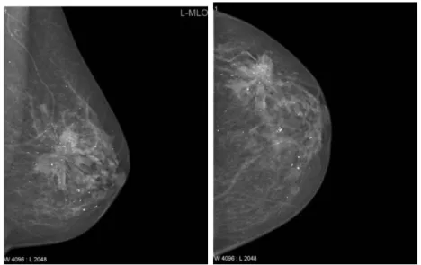
2-1 Two routine projects of mammograms: MLO (left) and CC (right). . 18 2-2 Measurements of the PNL line in CC and MLO views.[1] . . . 19 2-3 Visualization of positioning metrics for both views. . . 20

4-1 Annotation tool created for the purposes of this study for nipple de-tection. Stored coordinates are shown in the left hand corner of the tool. . . 30 4-2 RetinaNet model architecture. . . 32 4-3 Mask generation process for the pectoralis muscle shown above in

or-der: (a) histogram of pixel intensities (b) thresholding to create binary mask and finding bounding boxes (c) finding largest bounding box (d) rectangular region of pectoralis muscle (e) mask of pectoralis muscle. 34 4-4 U-Net model architecture. . . 35 4-5 Edge dataset creation preprocessing. Last image shows the output of

the pretrained HED network. . . 36 4-6 Process of finding the pectoralis muscle edge using a pretrained HED

network, mask generation thresholding techniques, and a curve fitting approach. From the top: (a) Thresholding technique used to find re-gion with muscle, (b) Output of edge detection only showing edge near muscle region, (c) Lines found in the edge detection output, (d) De-noising the boundary by removing pixels not in the lines, (e) Smoothing out the boundary through curve-fitting techniques, (f) Final boundary on the image. . . 37

4-7 Examples of poor edge outputs from the pretrained HED network. Breasts without clear boundaries or those with more tissue render the pretrained network useless in finding edges. . . 38 4-8 Examples of annotations around pectoralis muscle bottom edge and

top right points. . . 39

5-1 Results from trained retinanet on a test set of MLO and CC views. Images are not necessarily from the same patient. The corresponding score of the box is labeled beside the bounding box. . . 44 5-2 Visualization of IoU calculation. Green is ground truth bounding box

and red is predicted bounding box. Equations below. . . 44 5-3 Examples of IoU values on test set. Green is ground truth bounding

box and red is predicted bounding box. . . 45 5-4 Bounding box score and IoU value distributions on test set. . . 46 5-5 Example of an MLO projection, result from HED network, and the

corresponding ground truth. . . 47 5-6 Boundary from output of HED network. . . 48 5-7 Results from trained retinanet on MLO images to detect the

mus-cle bottom. The corresponding score of the box is labeled beside the bounding box. . . 48 5-8 Examples of IoU values on test set. Green is ground truth bounding

box and red is predicted bounding box. . . 49 5-9 Bounding box score and IoU distributions on test set. . . 49 5-10 Results from trained retinanet on MLO images to detect the muscle

top. The corresponding score of the box is labeled beside the bounding box. . . 50 5-11 Examples of IoU values on test set. Green is ground truth bounding

box and red is predicted bounding box. . . 50 5-12 Bounding box score and IoU distributions on test set. . . 51 5-13 Example showing the distance calculations from the nipple in mm. . . 52

5-14 Example showing PNL of the CC view. Distance is in mm. . . 53 5-15 Example of nipple detection in MLO projection. . . 54 5-16 Example showing PNL of the MLO view. Distance is in mm. . . 55 5-17 Example showing distance between pectoralis muscle bottom and PNL

in MLO view. . . 56 5-18 Example showing angle of the pectoralis muscle in the MLO view. . . 57 5-19 Sample metrics assessment. . . 59

A-1 Sample metrics assessment. . . 66 A-2 Sample metrics assessment. . . 67

List of Tables

4.1 CC view assessments . . . 40 4.2 MLO view assessments . . . 41

Chapter 1

Overview

Breast cancer affects millions globally. More than 3.8 million US women with a history of breast cancer were alive on January 1, 2019. [8] The risk of breast cancer in the United States is high: approximately 1 in 8 women (13%) was diagnosed with an invasive breast cancer in their lifetime, and 1 in 39 women (3%) will die from breast cancer. [11]

To achieve earlier breast cancer detection, screening x-ray mammography is rec-ommended by health organizations worldwide and has been estimated to decrease mortality risk by as high as 60%. Earlier detection allows for earlier treatment and prevention. Mammography is the only approved method for early breast cancer de-tection, and recent studies show it has saved up to 600,000 women since 1989. [15] Unfortunately, 15 − 30% of cancers are still missed.

Recent strides in deep learning methods to detect breast cancers in mammography have achieved impressive accuracy in cancer detection in an effort to empower radiolo-gists and augment them in the screening process. However, detection of breast cancer in these images is heavily dependent on quality images and optimal positioning of the breast. This study focuses on computational methods to assess proper positioning of the breast and image quality of mammograms to ensure proper diagnosis.

Chapter 2

Background

Mammography is the process of using low-energy X-rays to examine the breast for diagnosis and screening of breast cancers, with a goal of early detection, which is essential for reducing mortality. Quality of mammograms, the images produced in mammography-based screening, is important for diagnosis: research has shown a direct link between image quality and cancer detection. According to a study by Taylor et. al [16], positioning is crucial for diagnosis, as improper positioning and poor quality images can contribute to missed cancers. Inadequate positioning of the breast in mammography can result in undetected cancers and reduce the efficacy of mammography screening or lead to repeat examinations and added cost. In 2015, the American College of Radiology (ACR) found that of all clinical images deficient at the first attempt at accreditation, 92% were deficient in positioning. [3]

In order to prevent undetected breast cancers and repeat visits, the Food and Drug Administration (FDA) in the United States began to regulate mammography through the federal Mammography Quality Standards Act (MQSA) legislation. These guide-lines for mammographic image quality attempt to establish rules for mammographic practice for accreditation of clinical images, which involves assessing positioning and other image attributes.

There are two projections that are acquired as part of the standard imaging used for detection in mammography-based screening: the mediolateral oblique (henceforth referred to as MLO) and the craniocaudal (henceforth referred to as CC). These

images are taken in a single imaging encounter. The mammography technologist places the breast on a plate in front of an X-ray machine and take images of these projections for both the left and right breast. Each view has its own positioning metrics to assess the quality of the image. In Figure 2-1, we can see an example of each of the two views mentioned.

The radiologist often interprets the images taken by the technologist after the pa-tient has left the imaging facility; if positioning standards are not met in accordance to the MQSA, the radiologist will require additional screening and for the patient to return to the facility. This leads to inefficiencies for patient, radiologist, and technol-ogist in terms of increased cost and time, both valuable to all parties involved, and delays in examination and detection of breast cancers. Due to the importance of these positioning standards and the negative costs of improper positioning, it is apparent that automatic assessment of positioning and quality can greatly aid mammography-based screening. However, as mentioned in Chapter 1, though much attention has been focused on computer-aided detection of breast cancers, few studies have at-tempted to improve methods for automated positioning assessment of mammograms. This study aims to address that need.

2.1

Positioning Guidelines

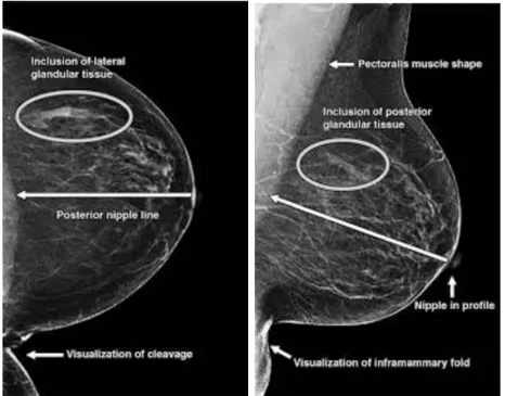
Positioning is often guided by landmarks in the images, the most important being the nipple (and whether the nipple is present in the image). The guidelines for the CC view are dependent on the existence of the nipple in profile. After determining whether the nipple is present, a line is drawn perpendicular to the nipple to the back of the breast. This line is known as the posterior nipple line (PNL). The Euclidean distance between the end coordinates of this line are compared to the PNL counterpart in the MLO view: the ‘1 cm’ rule then follows, which states that the PNL length from the MLO view must be within 1cm of the CC PNL.

The positioning guidelines for the MLO view are more involved. As in the CC view, first the nipple must be detected and localized. Additionally, the MLO view must include an adequate amount of the pectoralis major (pectoral) muscle, which is a key structure in the breast used to determine whether enough tissue is included in the mammogram. This muscle inclusion has been ranked as necessary for perfect or excellent images for some standards[13]. The PNL line then in the MLO view is drawn perpendicular to the pectoralis muscle and intersecting the nipple. This Euclidean distance must then follow the ‘1 cm’ rule as previously mentioned in relation to the CC PNL line. Volpara solutions lists this assessment at the top of the list of positioning challenges for mammograms[17]. Figure 2-2 shows examples of the PNL measurements for each projection.

The pectoralis muscle must also be positioned at nipple level. As shown in Figure 3, the shape of the muscle creates a triangle. The bottommost point of the triangle must be within 1 cm of the PNL line. In addition, the muscle must be at an appro-priate angle to ensure that enough of the muscle is visible on the mammogram. This angle can be defined as the angle between the hypotenuse and the longest leg of the triangle.

Figure 2-3: Visualization of positioning metrics for both views.

In addition to the positioning guidelines mentioned, other measures include image quality metrics. Sufficient compression while taking the mammogram is also impor-tant for image quality, and it is crucial to ensure that the images do not include any extra skin folds or creases.

2.2

Significance of Guidelines

Positioning standards for mammography exist to ensure that proper diagnosis can be made based on the routine mammography projections. Image quality and positioning has the biggest impact on a radiologist’s ability to accurately interpret mammograms. For example, a study comparing ultrasound to mammography found that 3% of

can-cers later detected on ultrasound were not included in the original mammographic images due to difficult anatomic location[5]. Technical problems and image quality have contributed to the delayed detection of 22% of screening-detected cancers and 35%of interval breast cancers. Though the technologist is responsible for performing the mammogram, the responsibility for correct positioning is shared by the technol-ogist and the interpreting physician as per the MQSA. Due to the existence of these stringent requirements for mammography, technologists must have a certain level of training and experience to avoid callbacks for screening, which can often be expensive and uncomfortable procedures for many women. The difficulty in adhering to guide-lines established to standardize mammograms is in large part due to the challenge of positioning.

Computational methods for assessment of positioning and image quality could aid technologists and radiologists alike in breast cancer diagnosis. According to Sweeney et. al, “... automated evaluation methods could better inform both research and validate image quality criteria for clinical application.”[13]. Therefore, the purpose of this study is, given the MLO and CC projections of a patient, to produce an automated report containing metrics on the visibility of the nipple, the lengths of the PNL lines, and the angle of the muscle, as described previously in Section 2.1.

Chapter 3

Related Work

In this section, we present related work from both a clinical and technical perspective. A lot of the early related work to this study focused on using traditional thresholding or statistical techniques from classical image processing to segment out regions of interest in the two projections described in the previous section (the pectoralis muscle and the nipple). Generally, segmenting out the pectoralis muscle as part of the MLO view is the most important task and the one that poses the greatest challenge. Recent advancements in computer vision have allowed for deep learning approaches to this task as well. Therefore, in summarizing work related to the subject of this study, we categorize it into two sections: thresholding and statistical techniques and deep learning techniques. Many previous studies focused on one or two subtasks of the assessment task (generally the segmenting of the muscle); few focused on generating a thorough automated assessment for both views of the mammograms. This study aims to bridge that gap by combining various techniques from previous work.

3.1

Thresholding and Statiscal Techniques

Much of the early work in this area focused on using statistical analysis and clas-sical image processing techniques to analyze breast images. For example, Kwok et. al. [7] presented an approach to automatic assessment of mammograms using the standard guidelines later mentioned earlier in this study. Their study focused on

im-age orientation, localization of the nipple, pectoralis muscle, and inframammary fold, and the curvature of the muscle. The study used entirely coordinate-system based geometric methods to evaluate the images by estimating a discrete function for the breast border and using this information to aid in analysis of the quality metrics. However, the study was entirely dependent on having knowledge of segmentation of the anatomic features of the breast (pectoralis muscle and nipple) before performing these geometric methods of evaluation, which was not automated.

In order to address the issue of automatic segmentation of these features, partic-ularly the muscle, studies then began to focus on extracting these regions through classical image processing. A study by Subashini et. al. [12] cites the most common approach: histogram-based thresholding in combination with morphological oper-ations in order to identify the muscle region. Though the paper was focused on assessing breast tissue density and not positioning quality, it showed that using these approaches could work with high accuracy for segmenting out the pectoralis muscle, and approach that is explored further in this study.

3.2

Deep Learning Techniques

Following the advancements in deep learning and computer vision, a new category of studies emerged using deep learning approaches to the subtasks presented in the task of automatic assessment. Rampun et. al. [9] proposed a deep learning approach to segmenting the pecotralis muscle by using an edge detection network to find the the pectoralis muscle line. This approach yielded high accuracy in detecting the muscle and is explored in in this study as part of the subtask of predicting the muscle line.

Gupta et. al. [2] also presented one such method by attempting to predict the PNL and pectoralis muscle line using an Inception-V3 network and the nipple location using an OpenCV implementation of a circle detection algorithm. The study produced an automated report that technologists can use to determine whether or not to reposition the breast during imaging. The study was able to find whether the lines intersected but did not include any numerical information regarding the length of the PNl line and

the angle of the muscle in the MLO view; however, this paper presents the approach closest to the proposed approach in this study.

Of the investigated related work, few have attempted to provide numerical assess-ments of positioning using a combination of deep learning and geometric methods. This proposed study attempts to take this approach in order to provide a numerical analysis of breast images.

Chapter 4

Methods

The purpose of this study was to address the need for assistance in evaluating the challenging tasks of breast positioning and image quality. The study focused on creating automated evaluation metrics as mentioned in Chapter 2 to aid proper cancer diagnosis. This section outlines the methods of the study, from the preparation of the data, to a description of the segmentation and detection tasks involved, to the computational geometric evaluation metrics.

4.1

Problem Statement and Summary

This section summarizes our problem statement. Given a mammogram of a patient, the projection of which (MLO or CC) will be previously known to us, we must deter-mine the location of the pectoralis muscle and/or the nipple. Following the detection of these significant landmarks in the image, we find the PNL lines on both projections for both the left and right breast of the patient. We can use these metrics to assess the mammogram quality.

4.1.1

Input and Output

Input: For each patient, we will be given the MLO and CC projection of one breast at a time in the form of Digital Imaging and Communications in Medicine (DICOM)

files. DICOM is the international standard to transmit, store, retrieve, print, process, and display medical imaging information. DICOM files contain the 1-dimensional pixel arrays corresponding to the grayscale image of the projection as well as relevant patient information, devoid of Personally Identifiable Information as per the Health Insurance Portability and Accountability Act (HIPAA). Both of these views will be combined for the assessment.

Output: The output will include metrics on the visibility of the nipple, the visual depictions of the PNL lines and their mathematical differences in lengths, and the angle of the pectoralis muscle for assessment. These metrics are described in greater detail in Section 4.6.

4.1.2

Assumptions

The following assumptions are in place when using this method:

• Each patient has four images for evaluation: two MLO projections (one for the left breast and one for the right) and two CC projections (one for the left breast and one for the right).

• The images are 2-dimensional.

• The images are grayscale.

• The images are not for-processing. Some of the DICOM images are marked "For Processing", which are generally all-black images of the projection.

• The pixel spacing values, or the scale from pixel to length in millimeters, will be known to us through the DICOM file.

4.1.3

Method Summary

First, we must determine a method to identify significant landmarks in the image. The images will be fed to trained Convolutional Neural Networks (CNNs), one for

determining the nipple and one for the pectoralis muscle. Then, geometric methods will be used to perform the analysis tasks. In order to build this system, the following steps are be taken:

1. Prepare a dataset containing the annotations for the nipple for each projection.

2. Prepare a dataset containing the pectoralis muscle region annotations for specif-ically the MLO projection.

3. Train a detection network to predict the location of the nipple.

4. Determine a method or train a network to predict the location of the pectoralis muscle.

5. Geometrically evaluate PNL lines for both projections, as well as other metrics as defined in Section 4.6.

6. Determine whether the analytical metrics are within standard guidelines for automatic assessment.

This study will first require preparation of the data to be able to perform the segmentation and detection tasks. The primary landmarks of interest are the nipple and the pectoralis muscle, which are both used to perform the geometric evaluation metrics mentioned in the previous section.

For the purposes of the segmentation and detection tasks, we needed to prepare an annotated dataset of the regions of interest. The dataset used for this study is the OPTIMAM Mammography Image Database from the National Health Service (NHS) in the United Kingdom. This dataset includes mammograms of patients in both of the routine projections (CC and MLO), but do not contain any annotations of the nipple or the pectoralis muscle. Therefore, these annotations are hand-engineered as part of this study. Due to the sensitive nature of the data, current existing annotation software and companies are not used for the purposes of this study to protect the privacy of the data.

4.2

Nipple Detection

This section details the methods used to detect the nipple. Nipple detection is a task that is necessary for both views of mammograms. In this section, we discuss the creation of the dataset as well as the deep learning techniques used to detect the nipple.

4.2.1

Nipple Dataset Creation

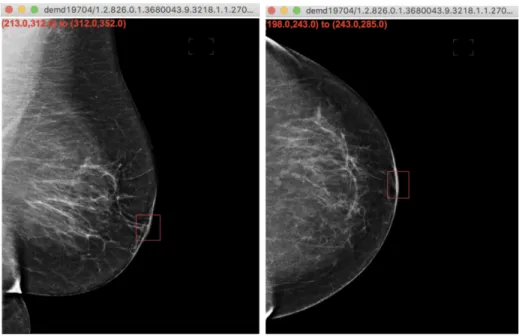
The first task is to find an optimal way to annotate the nipple in hundreds of breast images. Determining the location of the nipple falls under the category of object detection tasks. Therefore, our dataset needs to contain annotations of bounding boxes around the region containing the nipple in both the MLO and CC projections. In order to create these nipple annotations, we created our own an annotation tool to aid in drawing a bounding box around the nipple using the python package tkinter, shown in Figure 4-1. The tool allows the user to draw a rectangular shape around the nipple and stores the coordinates in the form of 𝑥1, 𝑦1, 𝑥2, 𝑦2.

Figure 4-1: Annotation tool created for the purposes of this study for nipple detection. Stored coordinates are shown in the left hand corner of the tool.

The annotations are stored in a csv file in the following format, where nipple is the name of the class of this bounding box:

image path, 𝑥1, 𝑦1, 𝑥2, 𝑦2,nipple

...

4.2.2

Nipple Detection Method

The detection of the nipple in the MLO and CC projections is a subset of the ob-ject detection problem in computer vision. For the purposes of this study, a fully-convolutional, detection-based model named RetinaNet [14], developed by Lin et. al., was used to detect the nipple.

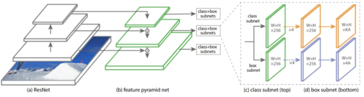
RetinaNet is one of the best one-stage object detection models that has proven to work well with dense and small scale objects, making it suitable for the nipple detection task on a mammogram, especially for denser breasts. RetinaNet was formed with a ResNet-50 backbone and by making two improvements to existing detection techniques - Feature Pyramid Networks (FPN) and Focal Loss [4]. The backbone computes the feature maps over the entire input image after every layer using a feature pyramid network. Then, a classification subnet is used to predict the possibility of object presence at each spatial location for each anchor box and object class by taking input feature map from a pyramid level and applying conv filters. Focal loss is used here, which is an improvement on cross-entropy loss for problems with class imbalance. This phenomenon can be seen in our breast images, which might suffer from foreground-background imbalance. Finally, a box regression subnet is applied, which outputs the object bounding box location from the anchor location. This entire process is shown in Figure 4-2.

For the purposes of this study, we trained a RetinaNet model on our dataset containing nipple annotations. Our training dataset included 636 images, made up of both MLO and CC projections, with corresponding bounding box annotations.

Figure 4-2: RetinaNet model architecture.

4.3

Pectoralis Muscle Segmentation

There are many methods that can be used to determine the location of the pectoralis muscle in the MLO projection of a mammogram, from traditional thresholding tech-niques to deep learning techtech-niques used to learn the region of interest. The next few sections will detail some of the methods that were used to determine the region in this study. Some traditional thresholding techniques were used to generate the dataset for the deep learning techniques.

4.3.1

Pectoralis Mask Generation

One method of finding the muscle mask is segmentation. While the task of finding the nipple in the breast images was an object detection task, finding this muscle can generally fall under a category of tasks called segmentation, which depends on a mask. Image segmentation involves partitioning the image into various parts called segments by grouping pixels that have similar attributes. In this task, rather than finding bounding boxes for an object of interest, we attempt to determine a pixel-by-pixel classification of the image.

For training purposes, annotating a mask around the pectoralis muscle by hand for hundreds of images is a lofty task. Therefore, classical image processing methods are applied to obtain a rough mask that can later be hand-tuned based on its accuracy. Since the pectoralis muscle is generally a triangular region in corner of the MLO images, we look for triangular regions of interest in the image. The muscle is also a

lighter shade than the rest of the image, motivating the use of classical morphological operations and thresholding techniques.

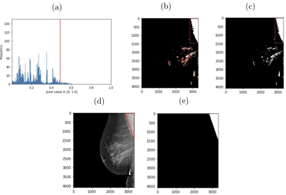
In this method, we first normalize the pixel values in the image between 0 and 1. Since the images are grayscale, we are only concerned with one channel. We then plot a histogram of all of the pixel values in the image to understand the distribution of pixel intensities. In Figure 4-3, we can see an example of pixel intensities plotted for one image. For the majority of images, most of the image is black and dark gray, with less than 50% of the image having higher intensity pixel values. This distribution varies across different densities of breasts, where a larger number of pixel intensities are higher due to dense fibroglandular tissue.

We then find the pixel intensity that is at the lower end of the high pixel intensities by finding the lowest pixel value of the intensities that are greater than 0.4. The image is thresholded based on this pixel value: any pixel value greater than this boundary is changed to a 1, and anything less to a 0. This creates a binary image highlighting lighter regions. This binary image might still contain noise from other lighter regions of the breast that are not part of the pectoralis muscle, especially if the breast has dense tissue. Therefore, we apply erosion and dilation, morphological operations to remove noise from the image. This makes it easier to find bounding boxes of regions of interest. We then find objects in the image by using OpenCV’s method to find contours, which draws boundaries around regions of the image that might have similar intensities. After finding rectangular bounding boxes of objects in the image, we find the largest bounding box that exists in the top region of the image. Using information from the DICOM, we can determine whether it is a left or right MLO image. This information can then be used to then find the triangle with the most high-intensity pixel values in this rectangular region and generate the triangular region of the pectoralis muscle.

These methods are used to generate masks for 70 images, as shown in Figure 4-3. Since this process can differ greatly across different breasts, especially denser breasts with more tissue, we were only able to generate 70 images.

(a) (b) (c)

(d) (e)

Figure 4-3: Mask generation process for the pectoralis muscle shown above in order: (a) histogram of pixel intensities (b) thresholding to create binary mask and finding bounding boxes (c) finding largest bounding box (d) rectangular region of pectoralis muscle (e) mask of pectoralis muscle.

4.3.2

Pectoralis Mask Segmentation

In order to find the segmentation mask, we used a Fully Convolutional Neural Network Model called U-Net, developed by Olaf Ronneberger et al. for Bio Medical Image Segmentation [10]. The architecture has two paths. The first path is the encoder path, which captures context in the image. The second is the decoder, which is used to enable precise localization using transposed convolutions. The architecture can be seen in Figure 4-4. For the purposes of this study, we train the U-Net with 70 MLO images and their corresponding masks.

4.4

Pectoralis Edge Detection

Another method used to determine the pectoralis muscle region in the MLO view depends on edge detection techniques. In this method, we combine a CNN with

mor-Figure 4-4: U-Net model architecture.

phological post processing steps. This CNN is derived from the HED (Holistically Edge Detection network) created by Xie et. al [18] and as studied by Rampun et. al. [9]. The original HED network was designed for edge detection purposes in natural images, which captures fine and coarse geometrical structures (e.g. contours, spots, lines and edges), whereas we are interested in only capturing the main boundary structures in mammograms, specifically pectoral boundaries. These contours can be detected using edge-based techniques as similar to the methods used to create the dataset for the pectoral mask segmentation task in Section 4.3.1; however, as previ-ously mentioned, these methods usually fail with denser breasts when fibroglandular tissue overlaps with the pectoralis muscle. Therefore, given poor results from the U-Net segmentation, we train our own HED network to detect only the muscle edge.

4.4.1

Pectoralis Edge Dataset Creation

In order to generate the muscle-edge dataset, we use a pretrained HED network in combination with the thresholding methods used to generate the segmentation masks to create our pectoralis muscle edges. We also flip all R-MLO images horizontally such that every image is a left MLO projection in order to avoid issues that may arise from the differing projections in the edge detection method.

We first threshold the image based on the lowest value of higher pixel values, as in the segmentation mask creation. However, in this method, we do not create a binary image; instead, we simply increase the contrast between the differing pixel regions to

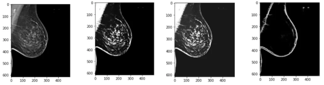
highlight the edges in the image Then we adjust the brightness and contrast levels of the image to make these edges more distinguishable, as seen in Figure 4-5.

Figure 4-5: Edge dataset creation preprocessing. Last image shows the output of the pretrained HED network.

Using a pretrained HED network, we find the initial edges of the image. We can see the variation of images and the outputs of the HED network in Figure 4-7. For denser breasts with more fibro-grandular tissue, we can see the pretrained edge detector has difficulty finding the specific muscle line, motivation for training our own edge detection network.

In order to find the edge of interest, we combine this with the mask generation techniques from 4.3. After finding the region of the muscle mask using the threshold-ing techniques, we can use that boundary to remove any edges from the output of the pretrained network that are not part of that region. We also remove any extraneous edges that were detected within the muscle itself. After that, we apply some mor-phological operations (erosion and dilation) to remove noise in the image. In order to smooth out the edge, we first find lines in the image. Using OpenCV, we can use the HoughLines command to find lines longer than 0.01 and remove any edges that are not part of these lines. We smoothen the line and any potential gaps that might exist in this edge by finding these gaps in the lines and using a polynomial fit to draw a curve between the points. We can see an example of the process for an image in Figure 4-6.

(a) (b)

(c) (d)

(e) (f)

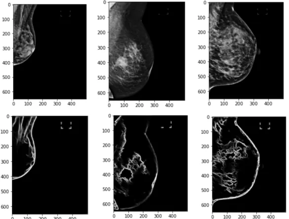
Figure 4-6: Process of finding the pectoralis muscle edge using a pretrained HED network, mask generation thresholding techniques, and a curve fitting approach. From the top: (a) Thresholding technique used to find region with muscle, (b) Output of edge detection only showing edge near muscle region, (c) Lines found in the edge detection output, (d) De-noising the boundary by removing pixels not in the lines, (e) Smoothing out the boundary through curve-fitting techniques, (f) Final boundary on the image.

We see that for a few images, this works well; however, the process fails for denser breasts or those without a defined boundary as seen in Figure 4-7, motivating the need for training our own network. We create a dataset of images and their muscle edge outlines for 120 images, fine tuning by hand as necessary, for training.

Figure 4-7: Examples of poor edge outputs from the pretrained HED network. Breasts without clear boundaries or those with more tissue render the pretrained network useless in finding edges.

4.4.2

Pectoralis Edge Detection

The HED network was developed by Xie et. al [18] as a deep learning approach towards edge detection. HED automatically learns rich hierarchical representations (guided by deep supervision on side responses) that are important in order to resolve the challenging ambiguity in edge and object boundary detection. We train the HED network on 120 MLO images and find the results on our test set to determine whether training our own HED network performs better in finding these msucle edges.

4.5

Pectoralis Muscle Points Detection

Finally, given that we only need the bottom edge and top right of the pectoralis muscle to generate the PNL line, as the line is drawn perpendicular to the nipple, the final method we investigate involves training the retinanet network on a dataset similar to the nipple detection dataset, but this time with bounding boxes around the end points of the triangular region of the muscle (i.e. bottom edge and top right).

4.5.1

Pectoralis Muscle End Dataset Creation

We use our original annotation tool developed for drawing bounding boses around the nipple for this task. Using this tool, we annotate the bottom of the muscle and the top right edge of the muscle in separate annotations such that they can be trained separately. We generate a dataset containing pectoralis bottom annotations for 260 images and top right annotations for 323 images. Examples are seen below in Figure 4-8.

Figure 4-8: Examples of annotations around pectoralis muscle bottom edge and top right points.

4.5.2

Pectoralis Muscle End Detection

We train the retinanet on 260 images to find the muscle bottom and 323 images to find the muscle top.

4.6

Analytical Methods

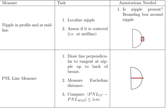
This section details the analytical methods used to assess the mammograms. Given the two models trained to predict the nipple and the pectoralis muscle region, we can now perform analytical tasks to determine whether a mammogram is of quality. Tables 4.1 and 4.2 detail the tasks that need to be performed.

Measure Task Annotations Needed

Nipple in profile and at mid-line

1. Localize nipple

2. Assess if it is centered (i.e. at midline)

1. Is nipple present? Bounding box around nipple

PNL Line Measure

1. Draw line perpendicu-lar to tangent at nip-ple up to back of breast. 2. Measure Eucledian distance. 3. Compare: |𝑃 𝑁𝐿𝐶𝐶 − 𝑃 𝑁 𝐿𝑀 𝐿𝑂| ≤ 1𝑐𝑚

Measure Task Annotations Needed

Nipple in profile 1. Localize nipple

1. Bounding box around nipple

PNL Line Measure

1. Draw line perpendicu-lar to pectoralis mus-cle and intersecting nipple.

2. Measure Eucledian distance.

3. Compare: |𝑃 𝑁𝐿𝐶𝐶 −

𝑃 𝑁 𝐿𝑀 𝐿𝑂| ≤ 1𝑐𝑚

Pectoralis muscle to nipple level

1. Roughly segment pectoralis muscle using triangle points as rough mask.

2. Determine distance of bottom edge of mask with respect to PNL line (within 1cm).

Pectoralis muscle angle

1. Roughly segment pectoralis muscle using triangle points as rough mask.

2. Calculate angle be-tween left edge of MLO image and line intersecting top right and bottom edge of muscle.

Chapter 5

Results

In this section, we present the experimental results of the methods presented in the previous chapter.

5.1

Nipple Detection

The retinanet network was trained on 636 MLO and CC images with ground truth annotations of nipple bounding boxes for 4 epochs, after which the classification and regression losses on the training data were nearly 0. The network was then tested on 270 images. The output of the model is a list of all possible bounding boxes of regions of interest in the image and the corresponding scores for each of the boxes. We plotted the bounding box with the highest score for each of the images and found great results. If a score is below 0.5, we ignore the box. Some of the bounding box outputs can be seen on a few MLO and CC projects in Figure 5-1.

The objectives of an object detection model are:

• Classification: Identify if an object is present in the image and the class of the object.

• Localization: Predict the coordinates of the bounding box around the object. In order the measure the performance of an object detection model, we need to evaluate the performance of both classification as well as localization of predicted

Figure 5-1: Results from trained retinanet on a test set of MLO and CC views. Images are not necessarily from the same patient. The corresponding score of the box is labeled beside the bounding box.

bounding boxes in the image. In object detection, a concept called Intersection over Union (IoU) is used to compute the intersection over union of the areas of the pre-dicted bounding box and the ground truth bounding box. An IoU of 1 would imply that the predicted the ground truth bounding boxes perfectly overlap. [6]

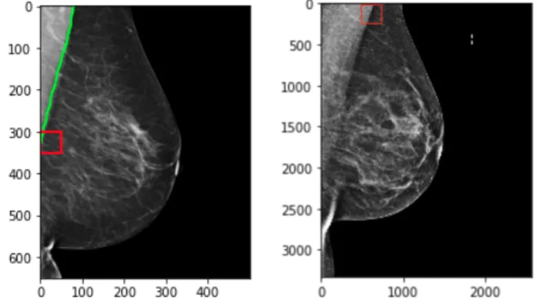
Figure 5-2: Visualization of IoU calculation. Green is ground truth bounding box and red is predicted bounding box. Equations below.

𝑔𝑎𝑟𝑒𝑎 = (𝑔𝑥2− 𝑔𝑥1+ 1) · (𝑔𝑦2− 𝑔𝑦1+ 1)

𝑝𝑎𝑟𝑒𝑎 = (𝑝𝑥2− 𝑝𝑥1+ 1) · (𝑝𝑦2− 𝑝𝑦1+ 1)

intersection area = (max(𝑔𝑥2, 𝑝𝑥2) − max(𝑔𝑥1, 𝑝𝑥1) + 1)·

(max(𝑔𝑦2, 𝑝𝑦2) − max(𝑔𝑦1, 𝑝𝑦1) + 1)

We calculate the IoU values for all of the test images. Some examples can be seen below in Figure 5-3. We can then set a threshold value for the IoU to determine how well the object detection model performed on this test set. Using a threshold of 0.5:

• If IoU ≥ 0.5, classify the object detection as True Positive(TP).

• If Iou < 0.5, then it is an incorrect detection; classify it as False Positive(FP).

• When a ground truth is present in the image and model failed to detect the object, classify it as False Negative(FN).

• True Negative (TN): TN is every part of the image where we did not predict an object. This metrics is not useful for object detection; hence we ignore TN.

Figure 5-3: Examples of IoU values on test set. Green is ground truth bounding box and red is predicted bounding box.

Figure 5-4 shows two graphs. The left is a violin plot showing the score distribu-tions of the highest and second highest bounding box depicted. The second is a violin plot showing the IoU values of the detected boxes. We can see that the majority of the detected boxes are valid (i.e. above 0.5).

We then use precision and recall as metrics to evaluate the performance. Precision is a metric that determines the probability that the bounding box predicted by the model is valid, whereas recall expresses the probability that the model is capable of detecting the bounding boxes that exist in the model. Using the following equations 5.1 and 5.2, we find a precision of 0.8346, implying that the probability that the detected bounding boxes are valid is pretty high. The recall is 0.9912, implying a very high probability the model is capable of detecting all of the bounding boxes.

Figure 5-4: Bounding box score and IoU value distributions on test set.

Given high precision and recall, we can conclude that the retinanet model is fairly accurate in detecting the nipple.

𝑃 𝑟𝑒𝑐𝑖𝑠𝑖𝑜𝑛 = 𝑇 𝑃

𝑇 𝑃 + 𝐹 𝑃 (5.1)

𝑅𝑒𝑐𝑎𝑙𝑙 = 𝑇 𝑃

𝑇 𝑃 + 𝐹 𝑁 (5.2)

5.2

Pectoralis Mask Segmentation

The U-Net resulted in poor results in detecting the mask of the muscle. After training for two epochs, the loss on the training set was extremely low, but every predicted image was black. A possible explanation for this lies within the class imbalance of the data: since the majority of a muscle mask is black, the model was probably predicting black for the majority of the predicted mask pixel values, resulting in high accuracy on the training set, but low accuracy on the test set. Due to this, we use a loss suitable for class-imbalanced data to penalize prediction of 0 (black) higher. However, the results were still very poor on the test data and therefore are not included in this section.

5.3

Pectoralis Edge Detection

The HED network was trained on 120 MLO images and their corresponding edge maps for 800 epochs, saving only the best weights, and tested on 20 images. After testing a couple of model weights on the images, we found epoch 247 to have the best edge detection result on the images, returning a mask which most closely aligned with the pectoralis muscle edge. An example of the output can be seen in Figure 5-5. We can see that there is still hand-engineering required to obtain the exact edge of the muscle from the output of this HED network.

Figure 5-5: Example of an MLO projection, result from HED network, and the corresponding ground truth.

Given the output of the model, we once again apply OpenCV’s method to find contours in the image and draw the largest contour, which will find the boundary close to the muscle. We then find the portions of the boundary that touch the muscle by only drawing the points on the inside of the contour, resulting in a rough outline of the boundary of the muscle. Though this method is able to detect the boundary on some of the images, we find that the majority of the outputs from the HED model will require hand-engineering to determine the exact boundary. These methods are often not easily transferable across the different types of breasts.

Figure 5-6: Boundary from output of HED network.

5.4

Pectoralis Muscle Points Detection

Since these tasks are also in the category of object detection tasks, similar analytical metrics are used to determine the performance of this model as used in Section 5.1.

5.4.1

Muscle Bottom

The retinanet network was trained on 260 MLO images with the corresponding bound-ing box of the bottom of the muscle. The network was then tested on 106 images. Some of the bounding box outputs can be seen in Figure 5-7.

Figure 5-7: Results from trained retinanet on MLO images to detect the muscle bottom. The corresponding score of the box is labeled beside the bounding box.

We again calculate the IoU values for the bounding boxes, as seen in Figure 5-8. The retinanet was unable to find the bounding box for some images, such as the example shown on the far right.

Figure 5-8: Examples of IoU values on test set. Green is ground truth bounding box and red is predicted bounding box.

Figure 5-9 shows two graphs. The left is a violin plot showing the score distribu-tions of the highest and second highest bounding box depicted. The second is a violin plot showing the IoU values of the detected boxes. We can see that the distribution for the IoU values here is much more varying, with a good number of invalid boxes.

Figure 5-9: Bounding box score and IoU distributions on test set.

We then use precision and recall as metrics to evaluate the performance. We find a precision of 0.5053, implying that the probability that the detected bounding boxes are valid is close to one half, which is not necessarily a great metric. The recall is 0.7833, implying that the probability that the model detected all of the bounding boxes is still high. Given moderate precision and high recall, we can conclude that the retinanet model is somewhat accurate in detecting the pectoralis muscle bottom. A potential explanation for the low precision of this model is the fact that some denser breasts might not have a well-defined muscle-bottom boundary, which made it difficult for the retinanet to detect the pectoralis muscle. It is possible that with more epochs and training data, this barrier can also be minimized.

5.4.2

Muscle Top

The retinanet network was trained on 323 MLO images with the corresponding bound-ing box of the bottom of the muscle. The network was then tested on 130 images. Some of the bounding box outputs can be seen in Figure 5-10.

Figure 5-10: Results from trained retinanet on MLO images to detect the muscle top. The corresponding score of the box is labeled beside the bounding box.

We again calculate the IoU values for the bounding boxes, as seen in Figure 5-11.

Figure 5-11: Examples of IoU values on test set. Green is ground truth bounding box and red is predicted bounding box.

Figure 5-12 shows two graphs. The left is a violin plot showing the score distri-butions of the highest and second highest bounding box depicted. The second is a violin plot showing the IoU values of the detected boxes. Once again, we see a high number of valid predicted boxes by the retinanet model.

We then use precision and recall as metrics to evaluate the performance. We find a precision of 0.9154, implying that the probability that the detected bounding boxes are valid is very high. The recall is 1.0, implying that the model was able to detect valid bounding boxes for all images. Given high precision and recall, we can conclude that the retinanet model is highly accurate in detecting the pectoralis muscle top.

Figure 5-12: Bounding box score and IoU distributions on test set.

5.5

Analytical Methods

In this section, we detail the analytical methods used to assess mammograms. Given the high accuracies from the retinanet models for detecting both the nipple and the pectoralis muscle points, we use the outputs of this model to aid us in finding the analytical metrics mentioned in Section 4.6.

For each projection, we have the following information:

• MLO: nipple bounding box, muscle bottom bounding box, muscle top bounding box

• CC: nipple bounding box

• Both: the row and column Pixel Spacing values in millimeters (mm) (𝑚𝑚𝑟𝑜𝑤, 𝑚𝑚𝑐𝑜𝑙),

or scale from pixel to length in millimeters

Using these values, we can determine the necessary metrics.

5.5.1

CC View

In this section, we discuss the methods used to obtain the necessary metrics for the CC projection.

5.5.1.1 Nipple in profile and at mid-line

The first task is to determine whether the nipple is in profile, which can be determined by whether the model is able to predict a bounding box for the nipple in the CC view. Given the bounding box coordinates, we can determine the coordinates of the nipple as the midpoint of the bounding box. Using (𝑥1, 𝑦1) as the top left of the bounding

box and (𝑥2, 𝑦2)as the bottom right of the bounding box, we can determine the nipple

coordinates as: 𝑛𝑥 = 𝑥1+ 𝑥2 2 (5.3) 𝑛𝑦 = 𝑦1+ 𝑦2 2 (5.4)

In order to determine whether it is at the midpoint, we can compare this to the top-most and bottom-most points of the breast. Using OpenCV, we can find the boundary points of the nipple, giving us these values. We can then use the following equations, with (𝑡𝑥, 𝑡𝑦) as the top-most point and (𝑏𝑥, 𝑏𝑦) as the bottom-most point:

top half = |𝑡𝑦 − 𝑛𝑦| * 𝑚𝑚𝑟𝑜𝑤 (5.5)

bottom half = |𝑏𝑦 − 𝑛𝑦| * 𝑚𝑚𝑟𝑜𝑤 (5.6)

5.5.1.2 PNL Line Measure

Given the coordinates for the nipple, we can easily draw the PNL by drawing a straight line from the nipple to the back of the breast in the CC projection. The direction can be determined from the position of the breast (L-CC or R-CC). With (𝑛𝑥, 𝑛𝑦)as the nipple coordinates and (𝑥, 𝑦) as the end-points of the PNL, we can use

the Eucledian distance to find the PNL length:

width = |𝑛𝑥− 𝑥| * 𝑚𝑚𝑐𝑜𝑙 (5.7)

height = |𝑛𝑦− 𝑦| * 𝑚𝑚𝑟𝑜𝑤 (5.8)

𝑃 𝑁 𝐿𝐶𝐶 =

√︁

width2_+height2 _(5.9)

Figure 5-14: Example showing PNL of the CC view. Distance is in mm.

5.5.2

MLO View

In this section, we discuss the methods used to obtain the necessary metrics for the MLO projection.

5.5.2.1 Nipple in profile

Similar to the CC projection, we can determine whether the nipple is in profile by whether the model is able to predict a bounding box for the nipple in the MLO view. Using (𝑥1, 𝑦1)as the top left of the bounding box and (𝑥2, 𝑦2) as the bottom right of

the bounding box, we can determine the nipple coordinates as:

𝑛𝑥 = 𝑥1+ 𝑥2 2 (5.10) 𝑛𝑦 = 𝑦1+ 𝑦2 2 (5.11)

Figure 5-15: Example of nipple detection in MLO projection.

5.5.2.2 PNL Line Measure

To find the PNL, we must now use the muscle bottom and top bounding box predic-tions. For the muscle bottom, the annotations were such that the bottom corner of the bounding box would be the bottom-most point of the muscle: the left bottom for L-MLO and right bottom for R-MLO. For the muscle top, the annotations were such that midpoint of the top line of the bounding box would be the muscle top boundary. We label the bottom point as (𝑏𝑥, 𝑏𝑦) and the top point as (𝑡𝑥, 𝑡𝑦). We refer to the

Given these muscle boundary points and the location of the nipple, we can now find the PNL. The PNL will be a perpendicular projection onto the muscle boundary from the nipple point. We can determine the muscle boundary as the line from (𝑏𝑥, 𝑏𝑦)

to (𝑡𝑥, 𝑡𝑦). Given these, we must find the equations of these two perpendicular lines,

the intersection of which will give us the endpoint of the PNL. We can once again use Eucledian distance to determine the length of the PNL:

𝑚1 = 𝑡𝑦 − 𝑏𝑦 𝑡𝑥− 𝑏𝑥 𝑚2 = −1 𝑚1 (5.12) 𝑏1 = 𝑡𝑦− 𝑚1· 𝑡𝑥 𝑏2 = 𝑛𝑦+ 𝑛𝑥 𝑚1 (5.13) 𝑥 = 𝑏2− 𝑏1 𝑚1− 𝑚2 𝑦 = 𝑚1· 𝑏2− 𝑏1 𝑚1− 𝑚2 + 𝑏1 (5.14) width = |𝑛𝑥− 𝑥| * 𝑚𝑚𝑐𝑜𝑙 (5.15) height = |𝑛𝑦− 𝑦| * 𝑚𝑚𝑟𝑜𝑤 (5.16) 𝑃 𝑁 𝐿𝑀 𝐿𝑂 = √︁ width2_+height2 _(5.17)

5.5.2.3 Pectoralis muscle to nipple level

Given the points of the PNL, we can determine the distance from the bottom of the muscle to the PNL as the shortest distance between the point and the line:

𝑚3 = 𝑦 − 𝑛𝑦 𝑥 − 𝑛𝑥 (5.18) 𝑏3 = 𝑦 − 𝑚1· 𝑥 (5.19) distance = −𝑚3· 𝑏𝑥+ 𝑏3− 𝑏𝑦 √︀𝑚2 3+ 1 ·√︁𝑚𝑚2 𝑐𝑜𝑙+ 𝑚𝑚2𝑟𝑜𝑤 (5.20)

Figure 5-17: Example showing distance between pectoralis muscle bottom and PNL in MLO view.

5.5.2.4 Pectoralis muscle angle

To determine the muscle angle, we can use the boundary points of the pectoralis muscle to draw a vertical line along the back of the muscle and the boundary line of the muscle itself. Given these points, we can determine the inverse tangent of the slope of the boundary line:

𝑚1 =

𝑡𝑦 − 𝑏𝑦

𝑡𝑥− 𝑏𝑥

(5.21) angle = 90 − arctan(𝑚1) (5.22)

Figure 5-18: Example showing angle of the pectoralis muscle in the MLO view.

5.5.3

Combination of Metrics

Given these metrics, we can now combine them to determine whether or not the mammograms are valid. For a patient, we obtain these metrics for both the MLO and CC projects for both breasts. Once we do that, we can determine the specific view-based metrics as well as the comparision of the PNL measurements of both views for assessment. We can see a sample assessment in Figure 5-19. More patient assessments can be found in Appendix A.

Chapter 6

Conclusion

In this section, we present the conclusion of the study.

6.1

Discussion of Contribution

This study proposed a novel method of assessing mammographic image quality using a combination of deep learning methods and geometric evaluation. Previous related work often focused heavily on obtaining the pectoralis muscle boundary for assess-ment. Early attempts of this task focused on using thresholding techniques; later the industry shifted to obtaining the muscle boundary using deep learning edge-detection techniques. However, no investigated related work took the approach of finding the pectoralis muscle boundary points through deep learning as shown in this study. The study found the approach of estimating the vertices of the pectoralis muscle landmark using a deep learning approach model to be the best approach and resulted in high precision and recall. Given recent advancements in deep learning for medical imag-ing, we predict these approaches will be favored over statistical approaches in future studies.

In this study, we demonstrated one method to assess mammographic quality based on quality assessment guidelines presented in the MQSA. Using the RetinaNet archi-tecture, we were able to predict the landmark points of the MLO and CC projections with high precision. The study combines the outputs of the deep learning model with

geometric methods to evaluate the necessary metrics. This combination ensures that the deep learning portion of this method remains end-to-end and can predict these landmark points with high accuracy, but does not rely solely on the RetinaNet to predict all of the numerical measurements, particularly the PNL line in the MLO view, as this could vary greatly among breasts of different densities. The purpose of this method was to demonstrate a proof-of-concept that evaluation of mammograms can be computer-aided. This study has shown that this combination of method can provide adequate feedback on mammographic image quality.

6.2

Limitations and Future Work

There are important limitations to the study to be discussed that can be addressed in future studies. The biggest one to discuss are regarding the annotations: nipple and pectoralis muscle bounding boxes and masks for these methods were annotated by the author of this study, an MEng student studying Computer Science at MIT. Though the author researched the localization of these landmarks heavily, since the author is not a licensed medical professional, we recommend that future studies use a radiologist to detail these annotations for highest accuracy in landmark detection. In addition, the images did not contain positioning and quality annotations, so accuracy of quality was not assessed numerically. The study recommends to obtain annotations on quality and more poorly positioned breasts.

Methods to detect the pectoralis muscle, especially the bottom of the region, can be better researched in future studies using data from different types of breasts in order to make the model more generalizable. It is important that the dataset contains breasts of various positions and densities to properly assess the performance of the model. We also recommend that the model be trained with more data and for longer number of epochs to allow for better predictions.

Finally, since the study has shown that a combination of deep learning and ge-ometric techniques can produce automated assessment of positioning and quality in a report, we propose applying this technique during an imaging session to provide

Appendix A

Figures

Bibliography

[1] Dr Francis Deng and Radswiki et al. Mammography views.

[2] Vikash Gupta; Clayton Taylor; Sarah Bonnet; Luciano M. Prevedello; Jeffrey Hawley; Richard D White; Mona G Flores; Barbaros Selnur Erdal. Deep learning-based automatic detection of poorly positioned mammograms to minimize pa-tientreturn visits for repeat imaging: A real-world application. 2020.

[3] Food and Drug Administration. Poor positioning responsible for most clinical image deficiencies, failures, 2017.

https://www.fda.gov/radiation-emitting-products/mqsa-insights/

poor-positioning-responsible-most-clinical-image-deficiencies-failures. [4] ArcGIS API for Python. How retinanet works? Technical report.

[5] Gatewood JB Hill JD Miller LC Inciardi MF. Huppe AI, Overman KL. Mam-mography positioning standards in the digital era: is the status quo acceptable? AJR Am J Roentgenol, 2017. ;209:1419–1425. doi: 10.2214/AJR.16.17522. [6] Renu Khandelwal. Evaluating performance of an object detection model. [7] Chandrasekhar R. Kwok, S.M. and Y. Attikiouzel. Automatic assessment of

mammographic positioning on the mediolateral oblique view. International Con-ference on Image Processing. Murdoch University Research Repository, 2004. [8] Lin CC et al. Miller KD, Siegel RL. Cancer treatment and survivorship statistics.

. CA Cancer J Clin, 2019.

[9] López-Linares K. Morrow P.J. Scotney B.W. Wang H. Ocaña I.G. Maclair G. Zwiggelaar R. Ballester M.A.G. Macía I. Rampun, A. Breast pectoral muscle segmentation in mammograms using a modified holistically-nested edge detection network. Medical Image Analysis, 2019.

[10] Brox T. Ronneberger O., Fischer P. U-net: Convolutional networks for biomed-ical image segmentation . 2015.

[11] American Cancer Society. Breast cancer facts figures 2019-2020. Atlanta: Amer-ican Cancer Society, Inc., 2019.

[12] Palanivel S. Subashini T.S., Ramalingam V. Automated assessment of breast tis-sue density in digital mammograms. Computer Vision and Image Understanding, 2018.

[13] Lewis SJ Hogg P et al. Sweeney, RI. A review of mammographic position-ing image quality criteria for the craniocaudal projection. Br J Radiol, 2018. 91:1082–1091.

[14] R. Girshick K. He T. Lin, P. Goyal and P. Dollár. Focal loss for dense object detection. 2017 IEEE International Conference on Computer Vision (ICCV). [15] Dean P.B. Chen T.H. et al Tabár, L. The incidence of fatal breast cancer

mea-sures the increased effectiveness of therapy in women participating in mammog-raphy screening. Cancer., page 125:515–523, 2019.

[16] Bouverat G Poulos A Gullien R Stewart E et al. Taylor K, Parashar D. Mam-mographic image quality in relation to positioning of the breast: a multicentre international evaluation of the assessment systems currently used, to provide an evidence base for establishing a standardised method of assessment. Radiography 2017.

[17] Kathy. Willison. Positioning challenge 4 – inadequate posterior nipple line (cc view).

[18] Tu Z. Xie S. Holistically-nested edge detection. 2015 IEEE International Con-ference on Computer Vision (ICCV), 2015.