Limit of a Function

Limit of a Function

Chapter 2

In This Chapter Many topics are included in a typical course in calculus. But the three most fun- damental topics in this study are the concepts of limit, derivative, and integral. Each of these con- cepts deals with functions, which is why we began this text by first reviewing some important facts about functions and their graphs.

Historically, two problems are used to introduce the basic tenets of calculus. These are the tangent line problem and the area problem. We will see in this and the subsequent chapters that the solutions to both problems involve the limit concept.

67

Limits—An Informal Approach

2.2

Limit Theorems

Continuity

2.4

Trigonometric Limits

Limits That Involve Infinity

Limits—A Formal Approach

The Tangent Line Problem

Chapter 2 in Review

y⫽ƒ(x) L

x®a^⫺ a x

y ƒ(x)®L

ƒ(x)®L

x®a^⫹

68 CHAPTER 2 Limit of a Function

2.1 Limits—An Informal Approach

Introduction The two broad areas of calculus known as differential and integral calculus are built on the foundation concept of a limit. In this section our approach to this important con- cept will be intuitive, concentrating on understanding what a limit is using numerical and graphical examples. In the next section, our approach will be analytical, that is, we will use al- gebraic methods to compute the value of a limit of a function.

Limit of a Function–Informal Approach Consider the function

(1) whose domain is the set of all real numbers except . Although f cannot be evaluated at because substituting for x results in the undefined quantity 0

0, can be calcu- lated at any number x that is very close to 4 . The two tables

f (x) 4

4

4 f (x) 16 x

4 x

show that as x approaches from either the left or right, the function values appear to be approaching 8, in other words, when x is near is near 8. To interpret the numer- ical information in (1) graphically, observe that for every number , the function f can be simplified by cancellation:

As seen in

, the graph of f is essentially the graph of with the excep- tion that the graph of f has a hole at the point that corresponds to . For x sufficiently close to , represented by the two arrowheads on the x-axis, the two arrowheads on the y-axis, representing function values , simultaneously get closer and closer to the number 8.

Indeed, in view of the numerical results in (2), the arrowheads can be made as close as we like to the number 8. We say 8 is the limit of as x approaches .

Informal Definition Suppose L denotes a finite number. The notion of approaching L as x approaches a number a can be defined informally in the following manner.

• If can be made arbitrarily close to the number L by taking x sufficiently close to but different from the number a, from both the left and right sides of a, then the limit of as x approaches a is L.

Notation The discussion of the limit concept is facilitated by using a special notation. If we let the arrow symbol represent the word approach, then the symbolism

indicates that x approaches a number a from the left, that is, through numbers that are less than a, and

signifies that x approaches a from the right, that is, through numbers that are greater than a. Finally, the notation

signifies that x approaches a from both sides,

in other words, from the left and the right sides of a on a number line. In the left-hand table in (2) we are letting (for example, is to the left of on the number line), whereas in the right-hand table .

One-Sided Limits In general, if a function can be made arbitrarily close to a number L

by taking x sufficiently close to, but not equal to, a number a from the left, then we write f (x) S L

as x S a

or lim (3)

xSa^ⴚ

f (x) L

. f (x)

x S 4

4 4.001

x S 4

x S a x S a

x S a

S f (x) f (x)

f (x) 4 f (x)

f (x) 4

x 4

y 4 x f (x) 16 x

4 x (4 x)(4 x)

4 x 4 x.

x 4

4, f (x)

f (x) 4

x 4.1 4.01 4.001

f (x) 8.1 8.01 8.001

x 3.9 3.99 3.999

f (x) 7.9 7.99 7.999 (2)

x y

4 y

8

16x² 4x

FIGURE 2.1.1 When x is near , is near 8

f(x) 4

59957_CH02a_067-120.qxd 9/26/09 5:20 PM Page 68

The number L

is said to be the left-hand limit of as x approaches a. Similarly, if can be made arbitrarily close to a number L

by taking x sufficiently close to, but not equal to, a num- ber a from the right, then L

is the right-hand limit of as x approaches a and we write

(4) The quantities in (3) and (4) are also referred to as one-sided limits.

Two-Sided Limits If both the left-hand limit and the right-hand limit exist and have a common value L,

then we say that L is the limit of as x approaches a and write

(5) A limit such as (5) is said to be a two-sided limit. See

. Since the numerical tables in (2) suggest that

(6) we can replace the two symbolic statements in (6) by the statement

(7) Existence and Nonexistence Of course a limit (one-sided or two-sided) does not have to exist. But it is important that you keep firmly in mind:

• The existence of a limit of a function f as x approaches a ( from one side or from both sides), does not depend on whether f is defined at a but only on whether f is defined for x near the number a.

For example, if the function in (1) is modified in the following manner

then is defined and but still See

. In general, the two-sided limit does not exist

• if either of the one-sided limits or fails to exist, or

• if and but

EXAMPLE 1

A Limit That Exists

The graph of the function is shown in

. As seen from the graph and the accompanying tables, it seems plausible that

and consequently lim

xS4

f (x) 6.

x

lim

f (x) 6 and lim

xS4^ⴙ

f (x) 6 f (x) x

2x 2

L

L

.

x

lim

f (x) L

,

x

lim

f (x) L

x

lim

f (x)

x

lim

f (x) lim

f (x)

x

lim

16 x

4 x 8.

f ( 4) 5, f ( 4)

f (x) • 16 x

4 x , x 4

5, x 4,

f (x) S 8 as x S 4 or equivalently lim

xS4

16 x

4 x 8.

f (x) S 8 as x S 4

and f (x) S 8 as x S 4

, lim

f (x) L.

f (x)

x

lim

f (x) L and lim

xSa^ⴙ

f (x) L,

x

lim

f (x)

x

lim

f (x) f (x) S L

as x S a

or lim

xSa^ⴙ

f (x) L

. f (x)

f (x) f (x)

2.1 Limits—An Informal Approach 69

x S 4

3.9 3.99 3.999

f (x) 5.41000 5.94010 5.99400

x S 4

4.1 4.01 4.001

f (x) 6.61000 6.06010 6.00600 Note that in Example 1 the given function is certainly defined at 4, but at no time did we substitute into the function to find the value of lim

xS4

f (x).

x 4

yƒ(x) L

x→a a x

y ƒ(x)→L

ƒ(x)→L

x→a

4 x y

8 y

16x² 4x ,

5, x 4

x4

y x²2x2

x y

6

4

FIGURE 2.1.2 as if and

only if as and

as xSa

f(x)SL xSa

f(x)SL

xSa f(x)SL

FIGURE 2.1.3 Whether f is defined at a or is not defined at a has no bearing on the existence of the limit of f(x)as xSa

FIGURE 2.1.4 Graph of function in Example 1

EXAMPLE 2

A Limit That Exists

The graph of the piecewise-defined function

is given in

. Notice that is not defined, but that is of no consequence when considering lim From the graph and the accompanying tables,

xS2

f (x).

f (2)

f (x) e x

, x 6 2 x 6, x 7 2

x S 2

2.1 2.01 2.001

f (x) 3.90000 3.99000 3.99900

x S 2

1.9 1.99 1.999

f (x) 3.61000 3.96010 3.99600

we see that when we make x close to 2, we can make arbitrarily close to 4, and so

That is,

EXAMPLE 3

A Limit That Does Not Exist The graph of the piecewise-defined function

is given in

. From the graph and the accompanying tables, it appears that as x approaches 5 through numbers less than 5 that Then as x approaches 5 through numbers greater than 5 it appears that But since

we conclude that lim does not exist.

xS5

f (x)

x

lim

f (x) lim

xS5^ⴙ

f (x),

x

lim

f (x) 5.

x

lim

f (x) 7.

f (x) e x 2, x 5 x 10, x 7 5 lim

f (x) 4.

x

lim

f (x) 4 and lim

xS2^ⴙ

f (x) 4.

f (x)

x S 5

5.1 5.01 5.001

f (x) 4.90000 4.99000 4.99900

x S 5

4.9 4.99 4.999

f (x) 6.90000 6.99000 6.99900

A Limit That Does Not Exist

Recall, the greatest integer function or floor function is defined to be the greatest integer that is less than or equal to x. The domain of f is the set of real numbers . From the graph in

we see that is defined for every integer n; nonetheless, for each integer n, does not exist. For example, as x approaches, say, the number 3, the two one- sided limits exist but have different values:

(8) In general, for an integer n,

EXAMPLE 5

A Right-Hand Limit

From

it should be clear that as that is

It would be incorrect to write since this notation carries with it the connotation that the limits from the left and from the right exist and are equal to 0. In this case does not exist since f (x) 1 x is not defined for x 6 0.

x

lim

1 x lim

1 x 0

x

lim

1 x 0.

x S 0

, f (x) 1 x S 0

x

lim

f (x) n 1 whereas lim

xSn^ⴙ

f (x) n.

x

lim

f (x) 2 whereas lim

xS3^ⴙ

f (x) 3.

lim

f (x)

f (n)

( q , q ) f (x) : x ;

x y

4

2

FIGURE 2.1.5 Graph of function in Example 2

FIGURE 2.1.6 Graph of function in Example 3

x y

5 7

5

x y

1

1 1 2 3 4 5 2

3 4

2

y _{⎣ ⎦}x

x x

y y x

FIGURE 2.1.7 Graph of function in Example 4

FIGURE 2.1.8 Graph of function in Example 5

The greatest integer function was discussed in Section 1.1.

59957_CH02a_067-120.qxd 9/26/09 5:20 PM Page 70

If is a vertical asymptote for the graph of then will always fail to exist because the function values must become unbounded from at least one side of the line

EXAMPLE 6

A Limit That Does Not Exist

A vertical asymptote always corresponds to an infinite break in the graph of a function f. In

FIGURE 2.1.9

we see that the y-axis or is a vertical asymptote for the graph of The tables

f (x) 1 > x.

x 0 x a.

f (x)

lim

f (x) y f (x),

x a

2.1 Limits—An Informal Approach 71

x S 0

0.1 0.01 0.001

f (x) 10 100 1000

x S 0

0.1 0.01 0.001

f (x) 10 100 1000

clearly show that the function values become unbounded in absolute value as we get close to 0. In other words, is not approaching a real number as nor as Therefore, neither the left-hand nor the right-hand limit exists as x approaches 0. Thus we conclude that does not exist.

EXAMPLE 7

An Important Trigonometric Limit

To do the calculus of the trigonometric functions , and so on, it is important to realize that the variable x is either a real number or an angle measured in radians. With that in mind, consider the numerical values of as given in the table that follows.

x S 0

f (x) (sin x) > x

sin x, cos x, tan x lim

f (x)

x S 0

. x S 0

f (x)

f (x)

x S 0

0.1 0.01 0.001 0.0001

f (x) 0.99833416 0.99998333 0.99999983 0.99999999

It is easy to see that the same results given in the table hold as Because is an

odd function, for and we have and as a consequence

As can be seen in

, f is an even function. The table of numerical values as well as the graph of f strongly suggest the following result:

(9) The limit in (9) is a very important result and will be used in Section 3.4. Another trigonometric limit that you are asked to verify as an exercise is given by

(10) See Problem 43 in Exercises 2.1. Because of their importance, both (9) and (10) will be proven in Section 2.4.

An Indeterminate Form A limit of a quotient , where both the numerator and the denominator approach 0 as is said to have the indeterminate form 0 0. The limit (7) in our initial discussion has this indeterminate form. Many important limits, such as (9) and (10), and the limit

which forms the backbone of differential calculus, also have the indeterminate form 0 0. >

lim

f (x h) f (x)

h ,

>

x S a,

f (x) > g(x) lim

1 cos x

x 0.

lim

sin x

x 1.

f ( x) sin ( x) x sin x

x f (x).

sin( x) sin x x 6 0

x 7 0

sin x x S 0

.

x x x

y ƒ(x)

ƒ(x) y1

x

FIGURE 2.1.9 Graph of function in Example 6

x y

ysinx x

1

FIGURE 2.1.10 Graph of function in Example 7

EXAMPLE 8

An Indeterminate Form

The limit has the indeterminate form 0 0, but unlike (7), (9), and (10) this limit fails to exist. To see why, let us examine the graph of the function For

and so we recognize f as the piecewise-defined function (11) From (11) and the graph of f in

it should be apparent that both the left-hand and right-hand limits of f exist and

.

Because these one-sided limits are different, we conclude that lim does not exist.

xS0

0 x 0 > x

x

lim

0x 0

x 1 and lim

xS0^ⴙ

0x 0 x 1 f (x) 0x 0

x e 1, x 7 0 1, x 6 0.

x 0, 0 x 0 e x, x 7 0 x, x 6 0

f (x) 0 x 0 > x.

>

lim

0 x 0 > x

Exercises 2.1

Fundamentals

In Problems 1–14, sketch the graph of the function to find the given limit, or state that it does not exist.

1. 2.

3. 4.

5. 6.

7. 8. lim

xS0

0x 0 x

lim x

xS3

0x 3 0

x 3

lim

x

3x lim x

xS1

x

1 x 1

lim

1 x 1 lim

Q ¹ 1

x R

lim

(x

1) lim

(3x 2)

9. 10.

11. where

12. where

13. where f (x) • x

2x, x 6 2

1, x 2

x

6x 8, x 7 2 lim

f (x)

f (x) e x, x 6 2 x 1, x 2 lim

f (x)

f (x) e x 3, x 6 0 x 3, x 0 lim

f (x)

lim

x

1 x

1 lim

x

x

NOTES FROM THE CLASSROOM

While graphs and tables of function values may be convincing for determining whether a limit does or does not exist, you are certainly aware that all calculators and computers work only with approximations and that graphs can be drawn inaccurately. A blind use of a cal- culator can also lead to a false conclusion. For example, is known not to exist, but from the table of values

one would naturally conclude that On the other hand, the limit (12) can be shown to exist and equals See Example 11 in Section 2.2. One calculator gives

The problem in calculating (12) for x very close to 0 is that is correspondingly very close to 2. When subtracting two numbers of nearly equal values on a calculator a loss of significant digits may occur due to round-off error.

2 x

4

1 4

.

lim

2 x

4 2 x

lim

sin (p > x) 0.

lim

sin (p > x)

lim x S a

x S 0 0.00001 0.000001 0.0000001 f (x) 0.200000 0.000000 0.000000

x

y y x

x

1 1

FIGURE 2.1.11 Graph of function in Example 8

x S 0 0.1 0.01 0.001

f (x) 0 0 0

.

59957_CH02a_067-120.qxd 9/26/09 5:20 PM Page 72

2.1 Limits—An Informal Approach 73

14. where

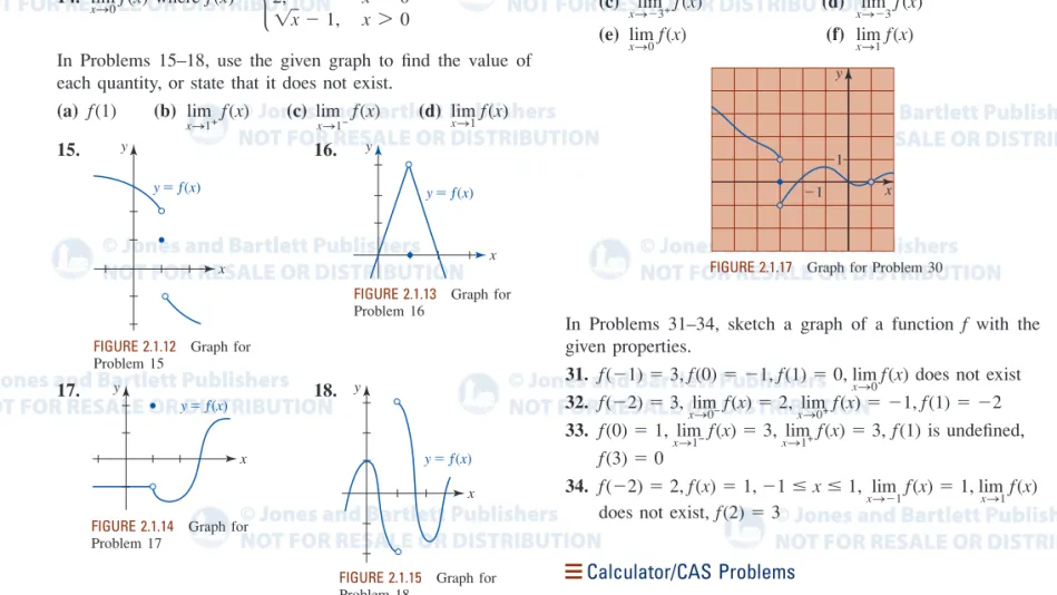
In Problems 15–18, use the given graph to find the value of each quantity, or state that it does not exist.

(a) (b) (c) (d)

15. 16.

17. 18.

In Problems 19–28, each limit has the value 0, but some of the notation is incorrect. If the notation is incorrect, give the cor- rect statement.

19. 20.

21. 22.

23. 24.

25. 26.

27. 28.

In Problems 29 and 30, use the given graph to find each limit, or state that it does not exist.

29. (a) (b)

(c) (d)

(e) (f) lim

xS4^ⴚ

f (x) lim

f (x)

lim

f (x) lim

f (x)

x

lim

f (x)

xS

lim

f (x)

lim

ln x 0

x

lim

2 9 x

0

lim

cos

x 0

x

lim

sin x 0

lim

2

: x ; 0

x

lim

: x ; 0

xS

lim

1 x 2 0 lim

11 x 0

lim

xS0

1

x 0 lim

xS0

1

x 0

lim

f (x) lim

xS1^ⴚ

f (x) lim

xS1^ⴙ

f (x) f (1)

f (x) • x

, x 6 0

2, x 0

1 x 1, x 7 0 lim

f (x)

30. (a) (b)

(c) (d)

(e) (f)

In Problems 31–34, sketch a graph of a function f with the given properties.

31. does not exist

32.

33. is undefined,

34.

does not exist,

Calculator/CAS Problems

In Problems 35–40, use a calculator or CAS to obtain the graph of the given function f on the interval [ , 0.5]. Use the graph to conjecture the value of or state that the limit does not exist.

35. 36.

37.

38.

39. 40.

In Problems 41–50, proceed as in Examples 3, 6, and 7 and use a calculator to construct tables of function values. Conjecture the value of each limit, or state that it does not exist.

41. 42.

43. 44.

45. 46.

47. 48.

49. 50. lim

xS2

x

8 x 2 lim

x

x 2 x 1

lim

c 6

x

9 6 1 x 2 x

9 d lim

1 x 2 x 4

x

lim

tan x lim x

xS0

x sin 3x

x

lim

1 cos x x

x

lim

1 cos x x

lim

ln x x 1 lim

61 x 612x 1 x 1

f (x) ln 0 x0 f (x) e

1 x

x f (x) 9

x [ ¹⁹ x 19 x ]

f (x) 2 1 4 x x

f (x) x cos 1 f (x) cos 1 x

x

lim

f (x), 0.5 f (2) 3

f ( 2) 2, f (x) 1, 1 x 1, lim

xS1

f (x) 1, lim

xS1

f (x) f (3) 0

f (0) 1, lim

xS1^ⴚ

f (x) 3, lim

xS1^ⴙ

f (x) 3, f (1) f ( 2) 3, lim

xS0^ⴚ

f (x) 2, lim

xS0^ⴙ

f (x) 1, f (1) 2

f ( 1) 3, f (0) 1, f (1) 0, lim

xS0

f (x)

x 1 1

y

lim

f (x)

x

lim

f (x)

x

lim

f (x)

xS

lim

f (x)

xS

lim

f (x)

x

lim

f (x)

y

x yƒ(x)

y

x yƒ(x)

y

x yƒ(x) FIGURE 2.1.12 Graph for Problem 15

FIGURE 2.1.13 Graph for Problem 16

y

x yƒ(x)

FIGURE 2.1.14 Graph for Problem 17

FIGURE 2.1.15 Graph for Problem 18

y

1 x 1

FIGURE 2.1.16 Graph for Problem 29

FIGURE 2.1.17 Graph for Problem 30

74 CHAPTER 2 Limit of a Function

2.2 Limit Theorems

Introduction The intention of the informal discussion in Section 2.1 was to give you an intuitive grasp of when a limit does or does not exist. However, it is neither desirable nor practical, in every instance, to reach a conclusion about the existence of a limit based on a graph or on a table of numerical values. We must be able to evaluate a limit, or discern its non-existence, in a somewhat mechanical fashion. The theorems that we shall consider in this section establish such a means. The proofs of some of these results are given in the Appendix.

The first theorem gives two basic results that will be used throughout the discussion of this section.

Theorem 2.2.1 Two Fundamental Limits (i) where c is a constant (ii) lim

xSa

x a lim

c c,

Theorem 2.2.2 Limit of a Constant Multiple If c is a constant, then

lim

c f (x) c lim

xSa

f (x).

Although both parts of Theorem 2.2.1 require a formal proof, Theorem 2.2.1(ii) is almost tautological when stated in words:

• The limit of x as x is approaching a is a.

See the Appendix for a proof of Theorem 2.2.1(i).

EXAMPLE 1

Using Theorem 2.2.1 (a) From Theorem 2.2.1(i),

(b) From Theorem 2.1.1(ii),

The limit of a constant multiple of a function f is the constant times the limit of f as x approaches a number a.

lim

x 2 and lim

xS0

x 0.

lim

10 10 and lim

xS6

p p.

We can now start using theorems in conjunction with each other.

EXAMPLE 2

Using Theorems 2.2.1 and 2.2.2 From Theorems 2.2.1 (ii) and 2.2.2,

(a) (b)

The next theorem is particularly important because it gives us a way of computing limits in an algebraic manner.

x

lim

(

x )

^lim

x (

) ^{. (} 2) 3.

lim

5x 5 lim

xS8

x 5 . 8 40

59957_CH02a_067-120.qxd 9/26/09 5:20 PM Page 74

2.2 Limit Theorems 75

Theorem 2.2.3 can be stated in words:

• If both limits exist, then

(i) the limit of a sum is the sum of the limits,

(ii) the limit of a product is the product of the limits, and

(iii) the limit of a quotient is the quotient of the limits provided the limit of the denominator is not zero.

Note: If all limits exist, then Theorem 2.2.3 is also applicable to one-sided limits, that is, the symbolism in Theorem 2.2.3 can be replaced by either or . Moreover, Theorem 2.2.3 extends to differences, sums, products, and quotients that involve more than two functions. See the Appendix for a proof of Theorem 2.2.3.

EXAMPLE 3

Using Theorem 2.2.3 Evaluate

Solution From Theorems 2.2.1 and 2.2.2, we know that and exist. Hence, from Theorem 2.2.3(i),

Limit of a Power Theorem 2.2.3(ii) can be used to calculate the limit of a positive integer power of a function. For example, if then from Theorem 2.2.3(ii) with

By the same reasoning we can apply Theorem 2.2.3(ii) to the general case where is a factor n times. This result is stated as the next theorem.

f (x) lim

[ f (x) ]

lim

xSa

[ f (x) . f (x)] ( ^lim

f (x) )( ^lim

f (x) ) ^L

^.

g (x) f (x),

x

lim

f (x) L, 10 . 5 7 57.

10 lim

xS5

x lim

xS5

7 lim

(10x 7) lim

xS5

10x lim

xS5

7

lim

10x lim

7

x

lim

(10x 7).

x S a

x S a

x S a

Theorem 2.2.3 Limit of a Sum, Product, and Quotient

Suppose a is a real number and and exist. If and , then

(i)

(ii) , and

(iii) lim

xSa

f (x) g(x) lim

xSa

f (x) lim

g(x) L

L

, L

0.

lim

[ f (x)g(x) ] ( ^lim

f (x) )( ^lim

g(x) ) ^L

^L

lim

[ f (x) g(x) ] lim

xSa

f (x) lim

xSa

g(x) L

L

,

x

lim

g(x) L

x

lim

f (x) L

lim

g(x) lim

f (x)

Theorem 2.2.4 Limit of a Power

Let and n be a positive integer. Then

lim

[ f (x) ]

[ ^lim

f (x) ]

^L

^.

lim

f (x) L

For the special case the result given in Theorem 2.2.4 yields

(1) lim

x

a

.

f (x) x,

76 CHAPTER 2 Limit of a Function

EXAMPLE 4

Using (1) and Theorem 2.2.3 Evaluate

(a) (b)

Solution

(a) From (1),

(b) From Theorem 2.2.1 and (1) we know that and Therefore by Theorem 2.2.3(iii),

EXAMPLE 5

Using Theorem 2.2.3 Evaluate

Solution In view of Theorem 2.2.1, Theorem 2.2.2, and (1) all limits exist. Therefore by Theorem 2.2.3(i),

EXAMPLE 6

Using Theorems 2.2.3 and 2.2.4 Evaluate

Solution First, we see from Theorem 2.2.3(i) that

It then follows from Theorem 2.2.4 that

Limit of a Polynomial Function Some limits can be evaluated by direct substitution. We can use (1) and Theorem 2.2.3(i) to compute the limit of a general polynomial function. If

is a polynomial function, then

In other words, to evaluate a limit of a polynomial function f as x approaches a real number a, we need only evaluate the function at :

(2) A reexamination of Example 5 shows that where is given by Because a rational function f is a quotient of two polynomials and , it follows from (2) and Theorem 2.2.3(iii) that a limit of a rational function can also be found by evaluating f at :

(3)

x

lim

f (x) lim

xSa

p(x) q(x) p(a)

q(a) . x a

f (x) p(x) > q(x) q(x) p(x)

f (3) 0.

f (x) x

5x 6, lim

f (x),

lim

f (x) f (a).

x a

c

a

c

a

. . . c

a c

. lim

xSa

c

x

lim

xSa

c

x

. . . lim

xSa

c

x lim

xSa

c

lim

f (x) lim

xSa

( ^c

x

c

x

. . . c

x c

)

f (x) c

x

c

x

. . . c

x c

lim

(3x 1)

[

^lim

(3x 1) ]

²

^1024.

lim

(3x 1) lim

xS1

3x lim

xS1

1 2.

lim

(3x 1)

.

lim

(x

5x 6) lim

xS3

x

lim

xS3

5x lim

xS3

6 3

5 . 3 6 0.

lim

(x

5x 6).

x

lim

5 x

lim

xS4

5 lim

x

5

4

5 16 .

lim

x

16 0.

lim

5 5

x

lim

x

10

1000.

lim

5 x

.

x

lim

x

f is defined at xa and this limit is f(a) d

59957_CH02a_067-120.qxd 9/26/09 5:20 PM Page 76

2.2 Limit Theorems 77

Of course we must add to (3) the all-important requirement that the limit of the denomina- tor is not 0, that is,

EXAMPLE 7

Using (2) and (3) Evaluate

Solution is a rational function and so if we identify the polynomials

and , then from (2),

Since it follows from (3) that

You should not get the impression that we can always find a limit of a function by sub- stituting the number a directly into the function.

EXAMPLE 8

Using Theorem 2.2.3

Evaluate

Solution The function in this limit is rational, but if we substitute into the function we see that this limit has the indeterminate form 0 0. However, by simplifying first, we can then apply Theorem 2.2.3(iii):

Sometimes you can tell at a glance when a limit does not exist.

lim

xS1

1

x

lim

(x 2) 1 3 . lim

xS1

1 x 2 lim

x 1

x

x 2 lim

xS1

x 1 (x 1)(x 2)

> x 1

lim

x 1 x

x 2 .

x

lim

3x 4

8x

2x 2 p( 1) q( 1)

7 4

7 4 . q( 1) 0

x

lim

p(x) p( 1) 7 and lim

xS1

q(x) q( 1) 4.

q(x) 8x

2x 2 p(x) 3x 4

f (x) 3x 4 8x

2x 2

x

lim

3x 4 8x

2x 2 .

q(a) 0.

cancellation is valid provided that x1 d

Theorem 2.2.5 A Limit That Does Not Exist

Let and . Then

does not exist.

x

lim

f (x) g(x) lim

g(x) 0

lim

f (x) L

0

PROOF We will give an indirect proof of this result based on Theorem 2.2.3. Suppose and and suppose further that exists and equals L

. Then

By contradicting the assumption that L

0 , we have proved the theorem.

(

^lim

g(x) ) ^{Q lim}

f (x)

g(x) R 0 . L

0.

L

lim

xSa

f (x) lim

xSa

Q ^{g(x) .} _g(x) ^{f (x)} R ^, g(x) 0,

x

lim

( f (x) > g(x)) lim

g(x) 0

lim

f (x) L

0

If a limit of a rational function has the indeterminate form as , then by the Factor Theorem of algebra must be a factor of both the numerator and the denominator. Factor those quantities and cancel the factor xa.

xa

xSa 0>0

78 CHAPTER 2 Limit of a Function

cancel the factor x5 d

limit exists d

EXAMPLE 9

Using Theorems 2.2.3 and 2.2.5 Evaluate

(a) (b) (c)

Solution Each function in the three parts of the example is rational.

(a) Since the limit of the numerator x is 5, but the limit of the denominator is 0, we conclude from Theorem 2.2.5 that the limit does not exist.

(b) Substituting makes both the numerator and denominator 0, and so the limit has the indeterminate form By the Factor Theorem of algebra, is a factor of both the numerator and denominator. Hence,

(c) Again, the limit has the indeterminate form 0 0. After factoring the denominator and canceling the factors we see from the algebra

that the limit does not exist since the limit of the numerator in the last expression is now 1 but the limit of the denominator is 0.

Limit of a Root The limit of the nth root of a function is the nth root of the limit whenever the limit exists and has a real nth root. The next theorem summarizes this fact.

lim

xS5

1 x 5 lim

x 5

x

10x 25 lim

xS5

x 5 (x 5)

>

0 6 0.

lim

xS5

x 5 x 1 lim

x

10x 25 x

4x 5 lim

xS5

(x 5)

(x 5)(x 1)

x 5 0 > 0.

x 5

x 5 lim

x 5 x

10x 25 .

x

lim

x

10x 25 x

4x 5 lim

x x 5

Theorem 2.2.6 Limit of a Root

Let and n be a positive integer. Then

provided that L 0 when n is even.

lim

2

f (x) 2

lim

xSa

f (x) 2

L, lim

f (x) L

An immediate special case of Theorem 2.2.6 is

(4)

provided when n is even. For example, .

EXAMPLE 10

Using (4) and Theorem 2.2.3 Evaluate .

Solution Since we see from Theorem 2.2.3(iii) and (4) that

When a limit of an algebraic function involving radicals has the indeterminate form 0 0, rationalization of the numerator or the denominator may be something to try.

>

x

lim

x 1

x 2x 10 lim

xS8

x [

^lim

x ]

x

lim

(2x 10) 8 ( 8)

6

6 6 1.

x

lim

(2x 10) 6 0,

x

lim

x 1

x 2x 10

lim

1 x [ ^lim

x ]

⁹

³

a 0

x

lim

2

x 2

a,

59957_CH02a_067-120.qxd 9/26/09 5:20 PM Page 78

EXAMPLE 11

Rationalization of a Numerator

Evaluate

Solution Because we see by inspection that the given

limit has the indeterminate form . However, by rationalization of the numerator we obtain

We are now in a position to use Theorems 2.2.3 and 2.2.6:

In case anyone is wondering whether there can be more than one limit of a function as x S a , we state the last theorem for the record.

f (x) 1

2 2 1 4 . lim

xS0

1 2 lim

xS0

(x

4) lim

xS0

2 lim

2 x

4 2

x

lim

xS0

1 2 x

4 2 lim

xS0

1 2 x

4 2

. lim

xS0

x

x

A 2 x

4 2 B lim

xS0

(x

4) 4 x

A 2 x

4 2 B lim

2 x

4 2

x

lim

xS0

2 x

4 2 x

. 2 x

4 2 2 x

4 2 0 > 0

lim

2 x

4 2lim

xS0

(x

4) 2 lim

2 x

4 2

x

.

2.2 Limit Theorems 79

this limit is no longer 0>0 d

cancel x’s d

Theorem 2.2.7 Existence Implies Uniqueness If lim exists, then it is unique.

xSa

f (x)

NOTES FROM THE CLASSROOM

In mathematics it is just as important to be aware of what a definition or a theorem does not say as what it says.

(i) Property (i) of Theorem 2.2.3 does not say that the limit of a sum is always the sum of the limits. For example, does not exist, so

.

Nevertheless, since for the limit of the difference exists

(ii) Similarly, the limit of a product could exist and yet not be equal to the product of the

limits. For example, and so

but

because lim does not exist.

xS0

(1 > x)

lim

Q ^{x . 1} _x R ( ^lim

x ) ^{Q lim}

1 x R lim

Q ^{x . 1} _x R lim

xS0

1 1 x > x 1, for x 0,

lim

c 1 x 1

x d lim

xS0

0 0.

x 0, 1 > x 1 > x 0

lim

c 1 x 1

x d lim

xS0

1 x lim

xS0

1 x lim

(1 > x)

lim x S a

We have seen this limit in (12) in Notes from the Classroom at the end of Section 2.1.