/
An Analysis of the Fundamental Constraints on
Low Cost Passive Radio-Frequency Identification System Design
by
Tom Ahlkvist Scharfeld
B.S., Mechanical Engineering (1998)
Northwestern University
Submitted to the Department of Mechanical Engineering
In Partial Fulfillment of the Requirements for the Degree of
Master of Science
at the
Massachusetts Institute of Technology
August 2001
© 2001 Massachusetts Institute of Technology
All rights reserved
MASSACHUSMiTS INSTITUTE OF TECHNOLOGY
DEC 1 02001
LIBRARIES
iAdROhwvL
Signature of Author.
...
...
...
....
...
Department of Mechanical Engin&r ing
August 21, 2001
C ertified by ...
/
... u...
...
Sanjay E. Sarma
Associate Professor of Mechanical Engineering
Thesis Supervisor
A ccepted by .... ...
.,. ...
Ain A. Sonin
Chairman, Department Committee on Graduate Students
An Analysis of the Fundamental Constraints on
Low Cost Passive Radio Frequency Identification System Design by
Tom Ahlkvist Scharfeld
Submitted to the Department of Mechanical Engineering On August 21, 2001 in partial fulfillment of the Requirements for the Degree of Master of Science
Abstract
Passive radio frequency identification (RFID) systems provide an automatic means to inexpensively, accurately, and flexibly capture information. In combination with the Internet, which allows immediate accessibility and delivery of information, passive RFID systems will allow for increased productivities and efficiencies in every segment of the global supply chain. However, the necessary widespread adoption can only be achieved through improvements in performance - including range, speed, integrity, and compatibility - and in particular, decreases in cost. Designers of systems and standards must fully understand and optimize based on the fundamental constraints on passive RFID systems, which include electromagnetics, communications, regulations, and the limits of physical implementation. In this thesis, I present and analyze these fundamental constraints and their associated trade-offs in view of the important application and configuration dependant specifications.
Thesis Supervisor: Sanjay E. Sarma
Title: Associate Professor of Mechanical Engineering
ACKNOWLEDGEMENTS
When I arrived at MIT two years ago, I had little background in the material covered in this thesis. I wish to thank my advisor, Sanjay Sarma, most of all, for allowing me to move into an entirely new domain; one in which there were many better equipped at MIT. Sanjay has allowed me tremendous flexibility and freedom in defining a topic and preparing my thesis. Over the past two years, through the multiple topics I have explored, I have learned a tremendous amount. I owe much of this to Sanjay. Meetings were always motivating. Though Sanjay has been, and will likely continue to be incredibly busy, he has always made himself available for meetings, emails, and phone calls, at home or on the road.
I must also thank Dan Engels. Where Sanjay provided the freedom, Dan provided the push. Had it not been for Dan, I would likely have allowed myself much less time to write. Discussions with Dan were always interesting and insightful. His extreme distaste for gates and functionality has been infectious. I would like to thank the others at the Auto-ID Center. Kevin Ashton was very helpful in providing the much needed and often ignored insight into the requirements of the end user community. Brooke Peterson, Tracy Skeete, and David Rodriguera provided the support to make the Center an exciting, productive, and friendly place to work.
I must also thank those outside of MIT and the Auto-ID Center whose insights were invaluable. The Alien Technology and Wave-ID team, including John Rolin, Roger Stewart, and Curt Carrender, provided the essential practical and industrial viewpoint. Through them, not only did I learn a great deal about the technology, but also its development. My brief encounters with Matt Reynolds and even briefer encounters with Peter Cole were more helpful than they might imagine.
Finally, I must thank my friends for making MIT a truly enjoyable place to be, my officemates for graciously accepting my constant presence for the last few months, my housemates for graciously accepting my constant absence for the last few months, and my family for supporting me in spite of not knowing what I was doing. Special thanks to Jean Ah Lee for thoroughly reading my thesis, Steve Buerger for offering to read my thesis, my Mother, in spite of her Swedish tongue, for suggesting a few corrections, my Father for painstakingly lumbering through my thesis, Jenny Scharfeld for reading the first paragraph, and Anna Scharfeld for checking to see how long it was.
TABLE OF CONTENTS
1 INTRO DUCTION ... 8
1.1 Introduction... ... ... 8
1.2 Brief H istory of R FID ... ... ... ... 9
1.3 Classifications of RFID Systems ... ... 10
1.3.1 Chipless versus Chip... ... ... 10
1.3.2 Passive, Semi-Passive, and Active... ... 11
1.3.3 Read-only and Read-write ... ... 11
1.4 Assumptions... .. ... ... ... 11
1.5 Specifications ... ... ... ... ... 11
1.5.1 P erform an ce ... ... 12
1.5.2 Cost and Size ... ... ... 13
1.6 Functions, Constraints and Organization ... 13
1.6.1 Components and their Functions... ... 13
1.6.2 Constraints and Organization... ... 15
2 ELECTROMAGNETICS AND ANTENNAS ... 16
2.1 Introduction... ... ... 16
2.2 Maxwell's Equations and Electromagnetics Fundamentals... 16
2.3 Antennas and Their Surrounding Regions ... 18
2.4 Impedance of Space, Antennas, and Circuits... 20
2.5 Coupling in the Near Field and Far Field ... 22
2.5.1 Near-field Coupling ... ... ... ... 22
2.5.1.1 Inductive Coupling... 22
2.5.1.1.1 Resonance and Q ... ... 25
2.5.1.1.2 Load Modulation ... ... 25
2.5.1.1.3 Voltage Available to Load... 26
2.5.1.2 Capacitive Coupling... 26
2.5.1.2.1 Resonance and Load Modulation ... ... 27
2.5.2 Far-field Coupling... ... 27
2.5.2.1 Antenna Parameters ... . ... 27
2.5.2.2 Transmission and Reception ... ... 29
2.5.2.3 Reader to Tag Transmission ... ... 29
2.5.2.4 Backscatter Modulation ... 31
2.5.2.4.1 Scattering ... ... ... 31
2.5.2.4.2 Scattering and Radar Cross Section... ... 31
2.5.2.4.3 Antenna Scattering... ... 32
2.5.2.4.4 Power Scattered and Power Received ... 34
2.6 Environmental Influences ... ... ... 34
2 .6 .1 L oss ... ... 35
2.6.1.1 Near-field Loss ... ... ... 35
2.6.2 Other Antennas ... 37
2.6.3 Temperature and Humidity ... ... 37
2 .7 Sum m ary ... 37
3 COM M UNICATIONS... 38
3.1 Introduction... ... ... ... ... 38
3.2 Com munications Process ... ... ... 38
3.3 Signal and Spectra Fundamentals ... ... 38
3.3.1 Time Averaging, Power, and RMS ... 39
3.3.2 Fourier and Spectra ... ... 39
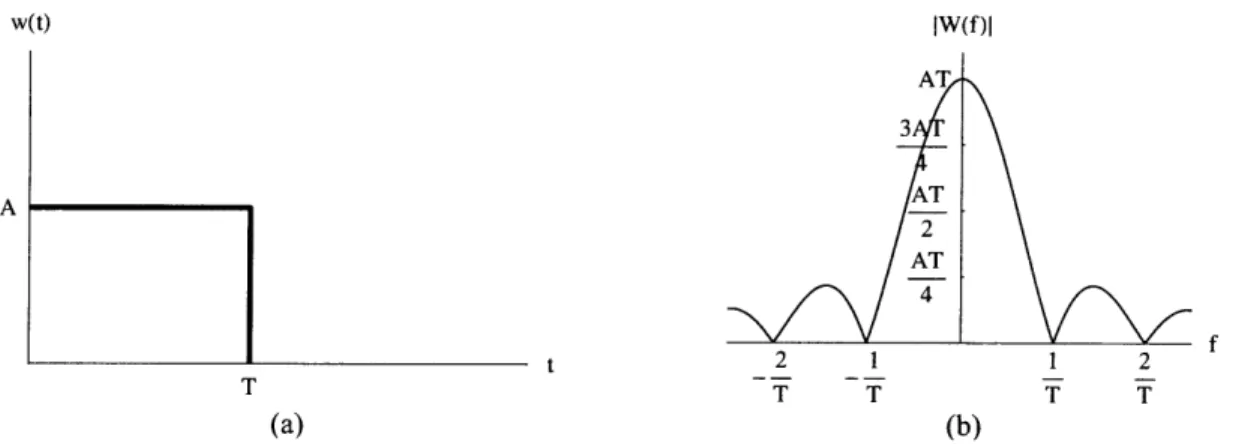
3.3.2.1 Rectangular Pulse... .... ... ... 40
3.3.2.2 Rectangular Pulse Train ... ... 41
3.3.2.3 Filtering ... ... 43
3.3.2.4 M odulation ... ... ... 44
3.3.2.5 Bandw idth ... ... ... 44
3.4 L ine C oding ... 45
3.4.1 Baseband Power Spectral Densities ... 47
3.4.1.1 NRZ... ... 49
3.4 .1.2 R Z ... ... 4 9 3.4.1.3 M anchester... ... ... 50
3.4.1.4 PW M and PPM ... ... ... .... 51
3.4.1.5 Miller and FMO ... 53
3.5 3.5.1 3. 3. 3.5.2 3. 3. 3.5.3 3.6 3.6.1 3.6.2 3.7 3.8 M odulation... ... 55
Reader to Tag Coding and Modulation... 56
5.1.1 Amplitude Shift Key (ASK) ... ... 56
5.1.2 Envelope Detection ... ... 57
Tag to Reader Modulation and Coding ... ... 58
5.2.1 Subcarrier ... ... .. ... ... 58 5.2.2 C oding ... ... 58 Spread Spectrum ... ... 59 Probability of Error ... ... ... 59 B urst N oise... ... ... 60 G aussian N oise... ... ... 60
Error Detection and Correction... ... 61
Sum m ary ... ... 62
4 REG ULATIO N S ... 63
4.1 Introduction... ... ... 63
4.2 Necessity of Common Allocations ... 63
4.3 Worldwide Structure of Regulatory Organizations... ... 63
4.3.1 ITU ... ... 63
4.3.2 R egional/N ational ... ... ... 64
4.4 Frequencies Available for RFID Use... ... 65
4.4.1 ISM ... ... 65
4.5
Radiation, Bandwidth, and Detection Specifications...
66
4.5.1
Field Strength and Power Conversion ...
67
4.5.1.1
Far-field
...
67
4.5.1.2
N ear-field ...
67
4.5.2
Bandw idth ...
68
4.5.3
D etection ...
68
4.6
Frequencies and Lim its ...
70
4.6.1
N ear-field Operation Frequencies ...
... 70
4.6.1.1
9 kH z - 135 kH z ... 70
4.6.1.2
6.78 M H z ...
72
4.6.1.3
13.56 M H z ...
72
4.6.1.4
27.12 M H z ...
73
4.6.1.5
40.68 M H z ... ... ...
...
...
... 74
4.6.2
Far-field O peration Frequencies ...
... 74
4.6.2.1
433.92 M H z
...
75
4.6.2.2
862-870 M H z ...
75
4.6.2.3
915 M H z ...
76
4.6.2.4
2.45 GH z ...
77
4.6.2.5
5.78 GH z ...
...
79
4.7
Sum m ary ...
79
5 PHYSICAL IMPLEMENTATION ... 81 5.1 Introduction... 81 5.2 Antennas ... 815.2.1
N ear-field ...
82
5.2.2
Far-field
...
83
5.2.2.1
D ipole A ntennas... 84
5.2.2.2
M icrostrip Patch A ntennas... ... 84
5.3
Integrated Circuit ...
85
5.3.1
Overall Architecture... 85
5.3.2
Components ...
85
5.3.2.1
Semiconductors and Transistors ...
86
5.3.2.2
Passive Com ponents ... ... 87
5.3.2.2.1
Resistors... 87
5.3.2.2.2
Capacitors ... 87
5.3.2.2.3
Inductors ... 88
5.3.2.3
Charge Pum ps ...
88
5.3.2.4
D iodes ... 88
5.3.2.5
O scillators ...
88
5.3.2.6
Phase-Locked Loops ...
88
5.3.2.7
D igital Circuits... 89
5.3.2.7.1
Flip-Flops and Latches ...
... 89
5.3.2.7.2 Shift Registers... 89
5.3.2.8
One-shots ...
89
5.3.2.9
M em ory
...
89
5.3.3
Integrated Circuit Pow er Consum ption...
90
5 .5 Su m m ary ... 9 1
6 COM M AND PROTOCOLS ... 92
6 .1 In trodu ction ... 92 6.2 Anti-Collision Overview... 92 6.2.1 Anti-Collision Analysis... ... 95 6.2.1.1 SuperTag . .... ... ... ... 95 6.2.1.2 Query-Tree Based ... ... 96 6.2.1.3 Results... ... 97 6.2.1.4 Com parison ... ... ... ... 98 6.2.2 Channelization ... ... ... ... 99 6.2.3 System Considerations ... ... 99 6.3 Com m ands ... ... 99
6.3.1 Commands and Bandwidth ... ... 99
6.4 Sum m ary ... ... ... ... 100
7 INFLUENCE OF CONSTRAINTS ON PERFORMANCE SPECIFICATIONS ... 101
7.1 Introduction... ... . .. .... ... ... ... 101
7.2 R ange ... ... .. ... 101
7.2.1 Field Strength, Orientation, and the Environment ... ... 102
7.2.2 Power Reception, Delivery, and Consumption ... 102
7.3 Speed and Integrity ... .... .... .. . ... ... ... 104
7.3.1 Data Rate.... ... ... ... 104
7.3.2 Identification R ate... ... .. ... . ... ... 105
7.4 Compatibility and Standardization.... ... 106
7.5 Sum m ary ... .. .. ... ... ... .. ... ... 107 8 CO NCLU SIO N ... 108 8.1 C onclusion ... ... .... ... ... 108 8.2 Future Work ... 108 REFERENCES ... 110 _ _
Chapter 1
INTRODUCTION
1.1
Introduction
Through the existing Internet infrastructure we have instant access to information from a wide variety of sources. It is the means by which this information is recorded which presents an obstacle. In many cases, information exists only in virtual form, whether it be in one's mind or in a machine. It may stay in virtual form. In other cases, however, information describes actual physical objects, states and events. Transforming this physically embodied information to virtual information so that people or machines may access it, presents a problem. Current solutions to this problem typically require manual intervention -people must observe and record. Not only can this be inefficient, but it can also result in inaccurate information. In other solutions, machines with sophisticated and complex vision and sensing systems may observe and record. Even for collecting the most basic information, however, such solutions are often expensive and complex, or require significant conditions and constraints. One potential solution to this problem is radio frequency identification (RFID). Through the attachment of transponders or tags to animate or inanimate objects, and an infrastructure of networked reading devices, physically embodied information can be automatically recorded. A class of RFID systems, passive RFID, allows wireless powering of these tags. Passive RFID systems have the potential to provide extremely low cost and somewhat less constrained automatic capturing of physically embodied information. Passive RFID systems, though capable of offering reduced operational constraints, have several fundamental constraints on their design. It is one objective of this thesis to analyze these constraints.
For a better understanding of this problem, we can consider the global supply-chain. It has been demonstrated that a manufacturer, distributor, retailer, and any other unit in a supply chain, merely knowing what they have and making that information available, will mean tremendous savings and increases in efficiencies [1]. Through the Internet and its associated infrastructure, the problem of delivering information has been solved; the problem of capturing information, however, has not. Current solutions require manual data entry, or manual scanning of barcodes. More sophisticated solutions include automatic scanning of barcodes, or sophisticated machine vision systems. The manual solutions can be costly, time consuming, and plagued by inaccuracies. The current automatic solutions can also be costly, complex, and often require significant constraints on the objects and their environment. Radio-frequency identification (RFID) systems are a potential solution.
Radio-frequency identification systems allow non-line of sight reception of an identification code assigned to an object. The identification code is stored in a tag consisting of a microchip attached to an antenna. A transceiver, often called an interrogator or reader, communicates with the tag. RFID systems alone are worthless. Though they may be able to collect identification codes, those codes must be assigned to an object and they must be made available to an accessible database. A network infrastructure that will support efficient and robust collection and delivery of information captured by RFID systems, or any other system capable of detecting identification codes, is currently being developed [2]. This system should support the capture, storage, and delivery of vast amounts of data robustly and efficiently.
Though each component of the entire system including tags, readers, host systems, databases, and network infrastructure, is equally important, it is the focus of this thesis to analyze and discuss tags, and the portions of the reader that interface directly with tags. The Internet and its associated infrastructure are proven and well developed technologies. RFID systems, though historically older than the Internet, are still relatively young and untested in their development for robust, high volume and low cost operation. Performance is currently satisfactory and constantly improving. Cost is still relatively high (minimum around $0.50/tag, and over $100.00/reader) and with increased improvements and adoption, should drop significantly in the near future. Technology innovations and new applications are driving increases in performance and decreases in costs. Standards, if properly designed, should drive adoption and further decreases in cost. For a better view of RFID and its direction, I will briefly review its history.
1.2
Brief History of RFID
RFID is merely a more recent term given to a family of sensing technologies that has existed for at least the past fifty years. The first commonly accepted use of RFID related technology was during World War II [3]. In their and their allies' aircraft, the British military installed transponders capable of responding with an appropriate identification signal when interrogated by a signal. This technology did not allow determination of exact identification, but rather if an aircraft was their own. This transponder technology, called identify friend or foe (IFF), has undergone continued development and later generations are still used in both military and civilian aircraft.
RFID, as we generally know it today, has also undergone significant development since the early aircraft transponder systems of World War II. In the 60s and 70s, in an effort to safely and securely track military equipment and personnel, various government labs developed identification technology. In the late 70s, two companies were created out of Los Alamos Scientific Laboratories to commercialize this technology. Initial applications included identification and temperature sensing of cattle [4]. In the early 80s railroad companies began using the technology for tracking and identification of railcars.
These early uses were typically at higher UHF frequencies (900 MHz/1.9 GHz). Through the 80s, several companies in the United States and Europe began developing technologies for operation at different frequencies, with different power sources, memories, and other functions. In the mid-to-late 80's, as the large semiconductor companies became involved, there was a shift towards performance improvement, size reduction, and cost reduction.
In the late 80s, and through the 90s, as performance improved, and size and cost decreased, new applications emerged. Some of these include automatic highway tolling, access control and security, vehicle immobilizers, airline baggage handling, inventory management and asset tracking, and the closely related smart-cards [5-8]. For continued adoption in applications demanding high performance, small size, and low cost, improvements in design and manufacturing must be achieved. Much work is continuing today and companies continue to emerge with innovative, low cost, and high performance technologies. With the advent of the Internet and increased development in information technology, RFID systems have been provided with the infrastructure necessary to achieve penetration into new applications.
For wide-scale global adoption of RFID technology, not only must performance improve and cost decrease, but also systems of one vendor must be compatible with those of another, and must additionally operate under both foreign and domestic regulations. Efforts to develop standards for RFID and various applications are continuing. Standards, though able to drive increased adoption and subsequent reduced costs, run the risk of stifling competition, innovation, and thus continued improvements in the technology.
It is a further objective of this thesis to understand the fundamental constraints on RFID systems for purposes of proper standards development.
1.3
Classifications of RFID Systems
Over the several stages of RFID system development, several types of systems have emerged. These can be classified in several ways. The term RFID implies a rather broad class of identification devices. All RFID systems have readers and tags. Readers capture the information stored or gathered by the tag. Readers are loosely attached to particular environments whereas tags are attached to objects. Because tags are attached to objects, they suffer the most stringent specifications related to performance, size, and cost. The various classifications of RFID systems are based around these specifications. One broad classification is that of "chip" versus "chipless" tags. Chip tags have an integrated circuit chip, whereas chipless tags do not. Another classification, which is a subset of chip tags, is that of passive, semi-passive, or active. Passive tags have no on-tag power source and no active transmitter, semi-passive tags have an on-tag power source, but no active transmitter, and active tags have both an on-tag power source and an active transmitter. Yet another classification is that of read-only or read-write. Read-only tags have either read-only, or write once read many memory. Read-write tags allow writing and re-writing of information. In this thesis, I will focus on read-only "chip" passive tags. I will briefly describe these classifications and justify this focus.
1.3.1 Chipless versus Chip
As our focus is on extremely low cost tags that provide the minimum of functionality - simply a read-only device with a permanent unique identification number - it might seem that chipless tags would be optimal. One would avoid the silicon costs and the intricate manufacturing process required for integrated circuitry. However, for two reasons, I will focus on the use of chips.
- The tag must hold enough memory to hold an identification number from a scheme designed to uniquely identify massive numbers of objects.
- The reader must be able to read multiple tags in its field.
In order to uniquely identify all manufactured items, a numbering scheme should allow for a sufficient number of unique codes. A length of 64-bits may be suitable in the near term, while 96-bits is optimal [9]. Most chipless tags at present allow up to 24 bits or less, though some may allow 64 bits [10]. These, however, come at a higher cost.
Because an ever increasing number of objects, ever decreasing in size, will be tagged, it is necessary that a reader be able to read multiple tags within its range and in close proximity to each other. At present, the best way to successfully accomplish this is through some intelligence on the tag itself. Methods of spatially isolating a single tag among many others, though potentially feasible, are not yet available. I will discuss the various multiple tag identification schemes in Chapter 7.
Though chipless tags show tremendous promise in achieving larger memories and improved anti-collision functions, and in the future, circuits may be printed directly onto non-silicon substrates, chip tags offer the most near-term promise in satisfying the demands of the majority of object tracking and identification
1.3.2 Passive, Semi-Passive, and Active
The difference between passive, semi-passive, and active tags is the power source and the transmitter. Passive tags have no on-tag power source and no on-tag transmitter. Semi-passive tags have an on-tag power source, but no on-tag transmitter. Active tags have both an on-tag power source and an active transmitter.
Active tags offer the best performance. Ranges can be on the order of kilometers and communications are fast and reliable. This comes at a high cost, however. Semi-passive tags offer increased operating ranges over passive tags (on the order of tens of meters) and because of their power source may allow increased functionality. These additions, however, also increase cost. Passive tags have ranges of less than 10 meters and are most sensitive to regulatory constraints and environmental influences. They however have the most potential for extreme low cost.
1.3.3 Read-only and Read-write
Any chip tag may be read-only or read-write. Typically though, only passive tags are read-only. Read-only tags have an identification code recorded at the time of manufacture, or when allocated to a particular object. Memory is either read-only memory (ROM), or write-once-read-many (WORM). I will discuss these memories further in Chapter 5.
Read-write tags may be written to many times throughout their life. They also typically have an identification code or serial number recorded at manufacture. Because a variety of information can be written, read-write tags offer additional functionality. This, however, comes at an increased cost.
Read-only tags offer the greatest potential for low cost, and in combination with a well-designed networked distributed database, provide essentially the same functionality as read-write tags.
1.4
Assumptions
Before discussing the specifications, I will reiterate the assumptions. I will assume that tags are read-only and passive. Range will typically be no more than 6 meters, and there is an infrastructure of readers, either at key locations or distributed throughout a facility. In addition, I will assume that there is a networked infrastructure through which identification codes unique to specific objects can be linked to information about those objects [2]. Identification codes will be logically partitioned with fields for a header, manufacturer code, product code, and serial number [9].
1.5
Specifications
As we have seen, through history, RFID applications have changed along with the technology itself. These applications each have their own specific demands. To properly analyze RFID technology, both for gaining an understanding of its functional characteristics, and for making improvements in design, we must evaluate its function on the basis of specifications. Because of the wide and varied applications, this is difficult. There are however some broad characteristics we should consider. These include cost, size, and performance. Performance concerns include reading range, speed, integrity of the communications, and compatibility between systems of different vendors and within differing worldwide regulation domains.
The more extreme and demanding near-term applications are those involving low-cost disposable and consumable items. Tagging of mail [11] and grocery items are two examples. In such applications, performance is important. Readers must be able to quickly read large numbers of tags at ranges on the order of meters in relatively unconstrained environments. Cost, however, is extremely important. Because the tagged items are consumable, and enormous numbers of items will be tagged, minute increases in the cost of a single tag will mean tremendous overall costs. Depending on the size of the object, size can also be extremely important. I will briefly discuss the performance, cost, and size specifications.
1.5.1 Performance
The main performance specifications include: range, speed, integrity, and compatibility. Exact specifications require knowledge of the exact application and configuration in which RFID systems are to be used. Though the broad application is low cost consumable item tagging, this can be subdivided into almost countless applications each with multiple configurations. For example, we can consider each unit in the supply chain including factories, distribution centers, retail stores, homes and waste management centers, and transportation between them.
In factories there are assembly, sorting, and shipping applications. Distribution centers might have receiving, sorting, picking, packing, and shipping applications. Retail stores might have receiving, sorting, and other inventory management applications. Homes may also have inventory management applications. Waste management centers might have sorting applications. Transportation providers and cross-docking providers will have additional inventory and sorting applications. Reverse logistics operations offer additional applications.
It is likely that if consumable items are tagged, the boxes and totes that hold them, the pallets that hold the boxes, and the containers that hold the pallets will also each be tagged. Pallet and container tags could likely be reusable, so cost constraints would not be so stringent. Boxes are fewer in number than the items inside, so cost demands will be more stringent than those for pallets, but not as stringent as those for items.
Given that containers, pallets, and boxes can be individually tagged and identified, their contents should be known. Identification of individual consumable items will occur at locations where they are no longer contained. Such situations occur in factories and distribution centers, but more frequently in stores, homes, and waste management centers. Applications in stores, particularly at checkout, are especially demanding. Readers and tags may have to cope with interference from other readers in the vicinity, and reflections or influences from metal and people in the environment. Large numbers of random distributions of items may need to be identified accurately and quickly. Maximum required range will likely need to be on the order of meters. Exact requirements, however, will depend on the desired configuration, of which a number exist. Readers may be installed around gates or portals, in mobile carts or containers, or stationed throughout an area. The environment may be somewhat constrained, or completely unconstrained - objects may need to be separated from other objects and passed through a reader individually, or simply carried in bulk at full walking speed through the door.
1.5.2 Cost and Size
Without doubt, from the standpoint of the end user, cost should be minimized. Given that tags are consumable and disposable, they are a recurring cost. Minute savings in the cost of a single tag will mean tremendous savings to the end user. Current targets are in the range of 5 cents or lower at significant volume. Minimization of cost at this scale presents major challenges to design. Every aspect of the system must be optimized first for low cost and second for performance - not only tags with their integrated circuit and antennas, but also all the methods used to fabricate, assemble, and apply the final product. Design must creatively exploit the fundamental constraints on the system.
Size, of course, is also extremely important. At the very minimum, tags should be smaller than the tagged object. The antenna will always be the constraining factor as tag microchips with dimensions less than 0.5 mm square have already been manufactured. Because performance, in particular range, is dependent on size and shape of antennas and antenna size is largely dependent on operating frequency, tags on very small objects will not be able to achieve the same performance of a tag with a larger antenna more suited to the operating frequency. At 5.8 GHz for example, an optimal antenna length is 2.5 cm, whereas at 915 MHz, an optimal antenna length is 16 cm. Antennas with lengths smaller than these optimal lengths may
still have suitable performance, however it will degrade. Blindly increasing frequency is not an option as there are other overriding constraints such as propagation, power transfer efficiency, and regulations. As with the other applications, size is highly application and configuration dependant. In some instances only extremely close range is required. In such cases, sizes may be very small.
Regardless, the main concerns remain cost, size, and performance related issues, including, range, speed, integrity and communications. It is these specifications, in combination with the fundamental constraints, that determine the ultimate design of the RFID system.
1.6
Functions, Constraints and Organization
Given the assumptions and the important specifications, we must consider the fundamental constraints. As the organization of this thesis is based around these constraints, I will summarize the organization in parallel with the constraints. First, however, it will be helpful to reconsider the components and functions of an RFID system.
1.6.1 Components and their Functions
In general, as shown in Figure 1.1, an RFID system consists of four main components: a host, a reader, multiple tags, and a channel through which the reader and tags communicate.
I will consider only the components of the system that interact directly with the function of the tags, namely the tag interface portion of the reader, the tags themselves, and the communications channel. The functions performed by these components along with the specifications and constraints that govern their design, are shown in Figure 1.2.
Figure 1.1: The four main components of an RFID system: host, reader, channel, and tags.
From Figure 1.2, we see that the operations of the tag and the reader are complementary. The internal operations of both the tag and the reader include the higher-level algorithms and command protocols necessary for identification of a single tag or multiple tags within the reading range of a reader. Commands are generally based around algorithms called anti-collision algorithms as they imply the ability to reduce the occurrence of multiple simultaneous, colliding responses to a query from the reader.
Figure 1.2: Functions of the reader, channel, and tag and their governing specifications and constraints. The interface operations involve the lower level functions necessary to satisfy the requirements of the higher-level commands. The reader must transmit power, information, and a clock. The information transmitted, is essentially what is required for the multiple identification, or anti-collision protocols. The clock is necessary for driving the digital circuitry of the tag. Depending on the frequency of operation, the clock is either generated directly from the carrier frequency, or through modulations of the carrier. The tag must receive and process the power, information, and clock from the reader-transmitted signal. After the higher-level internal processing of the received information, the tag may choose to transmit information, likely its identification code, or portions of it, back to the reader. In passive RFID, this is done through modulations of the reader's signal. The reader must, in turn, receive this information, and sned it back to the higher-level internal functions.
1.6.2 Constraints and Organization
The design and implementation of these various functions is determined by both the specifications and fundamental constraints. These constraints include the electromagnetics and communications, which define the methods by which the tag and reader can communicate, and the regulations and hardware constraints, which impose limits on these methods.
In Chapter 2, I will discuss the electromagnetic fields and waves that link the reader to the tag. I will describe how they are created by antennas and how their characteristics and behavior vary with operating frequency and distance from the antenna. I will describe how RFID systems exploit these characteristics to achieve power and communications coupling. Finally, I will cover the various environmental influences on the behavior of fields and waves, and the coupling between reader and tag.
In Chapter 3, I will discuss the communications between the reader and tag and the theory that describes it. I will discuss and analyze the characteristics of the various coding and modulation schemes commonly used in RFID. I will consider detection methods and concerns related to the integrity of communications
and error detection.
In Chapter 4, I will consider the regulations that govern both the electromagnetics and communications. I will consider regulations imposed by bodies in three different regions of the world, Europe, the United States, and Japan. I will discuss their various methods of specifying regulations and the implications this has for RFID systems.
In Chapter 5, I will discuss constraints related to physical implementation of the hardware. I will discuss those properties of antennas that affect performance, cost, and size. I will also consider the integrated circuit and how its design and implementation affects performance and cost.
In Chapter 6, I will discuss and analyze anti-collision methods and the command protocols necessary to drive the identification of multiple tags within the range of a reader.
In Chapter 7, I will relate the fundamental constraints to the important performance specifications, and discuss their interactions.
Chapter 2
ELECTROMAGNETICS AND ANTENNAS
2.1
Introduction
In RFID systems, readers are linked to tags by electromagnetic fields and waves occupying or propagating through the environment. In order to understand and design these systems we must understand how these fields and waves are created, manipulated, and received. In this chapter, I will review the principles and behaviors of electromagnetic fields and waves. We seek to understand,
- How fields are created, their size, available power, their variation with range, angle, orientation, and polarization, and how they are transmitted and received.
- How antenna type, size, and shape affect the properties of the field.
- How we can maximize the reception of power and information through tuning and matching. - How reactive and radiating link conditions vary with the channel and its environment.
These issues will aid us in understanding the physical constraints on RFID systems and the fundamentals governing their function. In addition, they will help us in understanding other fundamental constraints on RFID systems, including communications theory, and regulations. In the end we will consider how these various factors influence performance and cost.
2.2
Maxwell's Equations and Electromagnetics Fundamentals
When a single charge emitting static electric field lines is accelerated in some direction, an electric field is radiated. If that charge is continuously oscillated it will radiate a continuously oscillating electric field. A time and space varying electric field has an associated magnetic field. Maxwell's equations describe the behavior of these electromagnetic fields at every point in space and instant in time relative to the position and motion of charged particles [12]. We can represent these equations in time-harmonic (sinusoidal) form with frequency co, through the relationship a/lt = -jot:
VxE = jeoB (2.1)
Vx H = J - jcoD
(2.2)
V-D = p (2.3)VB
= 0 (2.4) where: E = electric field (V/m) H = magnetic field (A/m)B = magnetic flux density (T) D = electric displacement (C/m2)
J = electric current density (A/m2)
p = electric charge density (C/m3)
The continuity equation for the conservation of charge and current is given as
jcwp + V -J = 0 (2.5)
Together with Maxwell's equations, they form the fundamental equations of electromagnetics.
The time averaged power per unit area delivered through a surface by electric and magnetic fields is given by Poynting's vector:
S= Re{ExH*} (2.6)
where H* is the complex conjugate of H, and S is a power density having units of W/m2
.
In a region with no charge or current densities, an electric field, coupled with and orthogonal in polarization to a magnetic field, will propagate through a given medium in a direction perpendicular to both fields. This is an electromagnetic wave. An antenna is designed to radiate electromagnetic fields and waves.
In further discussion we will use several parameters to describe fields and waves. These parameters can be given in general form for describing interactions with any material. We will focus on those for loss-less media and free-space. The free-space wavenumber is given by
ko = oeo 0 _ = 2= = f= (2.7)
where:
c = speed of light 3 3x10⁸(m/s)
Eo = free space permittivity = 8.8542x 10⁻¹² (F / m)
Y
0 = free space permeability = 4r x 10- 7 (H / m)The permittivity relates the electric field E to the electric displacement D through D = EoE. The permeability relates the magnetic field H to the magnetic flux B through B = /oH.
Another useful parameter is the free-space impedance
770 =-
r(2.8)
0
Through the fundamental equations of electromagnetics and these various parameters, we can understand how field and waves are created.
2.3
Antennas and Their Surrounding Regions
For a better sense of the relationship between electromagnetic fields and waves, it is helpful to examine how they are formed by an antenna. We can derive the electric and magnetic fields created and radiated by any antenna using Maxwell's equations. For purposes of illustration, we will consider two antennas considered to be electrically small in that their maximum dimension is much less than the wavelength of oscillation. We will consider the ideal dipole, also known as a Hertzian dipole, and the small loop [13]. The ideal dipole is an infinitesimal element that carries current with a uniform amplitude and phase over its length. The small loop is a closed current loop with a perimeter of less than about a quarter of the oscillation wavelength. The small loop is the magnetic dual of the electric ideal dipole.
(a) (b)
Figure 2.1: (a) Ideal dipole and (b) small loop.
A general approach to deriving the radiated electric and magnetic fields involves first calculating a vector potential based on the current density. The electric field is found from the vector potential and the magnetic field is subsequently found from the electric field. Fields created by an oscillating ideal dipole with length dl can be written as [14]
Id
o12
2c[
11
-j- r4r
22cos6 I+
eIp
r
e
4r (j/3r) 2 (j3r)3 eF
(2.9) di 2L
1 1 (10 HH=
Id sinO spr 1 1 r-
e-j
(2.10) 4•r j/3r (jpr)Examining the electric and magnetic field equations, one should note the dependence on distance r from the antenna. When fir << 1 (or, r << A/2n), the third order terms will dominate. At this distance, the
electric field strength decays as 1/r3, and the magnetic field strength decays as 1/r2. We will refer to this region as the near-field.
When the distance r is much greater than 2/2ir, the first order terms dominate, and both the electric field
and magnetic field strengths decay as 1/r. We will refer to this region as the far-field.
Examining these equations further, we notice that in the near-field where fir << 1, not only does the third order term dominate, but e-•pr also approaches 1. The electric and magnetic fields reduce to
E
"=
j
4
3 0 (2cos6r+sin
)
(2.11)
Id .
H"'
=
s2
ine8
(2.12)
Beyond the dissimilar relationship with distance r indicating dissimilar decay, we note that the electric field is imaginary, indicating it is 2/4 (90 degrees) out of phase with the magnetic field. This is an indication of a reactive field - energy is essentially stored and released between the two fields. Evaluating the Poynting vector for this case further reveals that there is no real power flow. The electromagnetic fields in the near-field are essentially decoupled from each other and quasi-static. Further simplification will reveal that the small dipole is essentially behaving as a static electric dipole. In considering the far-field where fir >> 1, the first order terms dominate and the field equations reduce to
Idf -j inr
E = j - ioPe' sin 0 0 (2.13)
41r
H" =
j
Pejpr sinO9 (2.14)41 r
We immediately see that the electric and magnetic fields are in phase, orthogonal in polarization, and related in magnitude by E/HO-=77o, the intrinsic impedance of free space. Both fields decay as 1/r.
Evaluation of the Poynting vector reveals a real power density, indicating propagation through a surface. The electromagnetic fields in the far-field constitute an electromagnetic wave.
We can also consider the fields for a small loop antenna,
Icd £1 _ 1 _
E=
0 2jr
(2.15) E4•r
sin0 jPr + ejr) S 4I
1 + 1 Id 2sinO
+
j+
r
-jr4
jp' r (jr)
.
3The near-field components are
Id?
E"a
=
2 0sin 0
(2.17)
HId=
(2cosOr+sinO
)
(2.18)
and the far-field components are
H 1
j
pejr sin0O
(2.19)
Id
£
Ef
= -j ro0Pe
-j'sin
p
(2.20)
4w r
Noting the similarities between the ideal dipole and the small loop field equations, we see that the small loop is the dual of the ideal dipole.
There is yet another region is of concern, often called the Rayleigh region. In this region, it becomes reasonable to approximate a spherical electromagnetic wave as a uniform plane wave. Plane waves are those with an electric field with the same direction, magnitude, and phase in infinite planes, perpendicular to the direction of propagation. They do not exist in practice, as they would require infinitely sized sources. However, at a distance far enough from the source, this approximation becomes reasonable. This region is given by
2D
2r
>
(2.21)
where r is the distance from the antenna, and D is the length of a radiating line source. When we discuss electromagnetic waves, we will not only assume we are in the far-field, but also in the Rayleigh region. In addition to understanding the relationship between electromagnetic fields and waves, we also see that electromagnetic fields exhibit radically different behavior in the near-field zone as compared with the far-field zone. In the near-far-field, far-fields are reactive and quasi-static, while in the far-far-field they constitute radiated waves. This result is particularly important to RFID systems. Those systems operating at lower frequencies where the near-field encompasses the operating range, must achieve coupling through the quasi-static fields. RFID systems operating at higher frequencies typically operate in the far field and achieve coupling through electromagnetic waves.
We should note that the transition point between near-field and far-field is actually dependent on the antenna geometry. However, we will use the transition point of 2/27 as the standard definition.
2.4
Impedance of Space, Antennas, and Circuits
Before further analyzing the behavior of RFID systems operating in the near-field and far-field, it will be helpful to discuss the concept of impedance as it relates to free-space, antennas, and circuits. In general, impedance describes the relationship between an effort and a flow. In electromagnetic field and wave theory, impedance is the relationship between the electric field and the magnetic field.
E
Z = (2.22)
H
In an antenna or electrical circuit, it is the relationship between the voltage and the current.
V
Z = -(2.23)
I
Regardless of domain, it is an extremely useful parameter capable of characterizing the behavior of fields and waves, radiation and reaction of an antenna, and power transfer between an antenna, transmission line, and load.
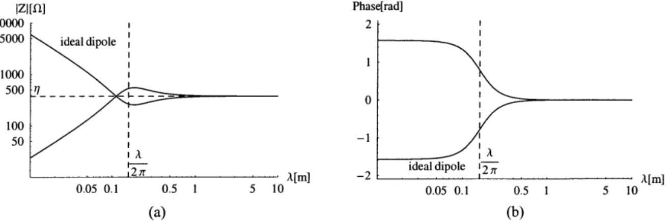
Figure 2.2a shows the magnitude of the free space impedance of the fields generated by both an ideal dipole, and a small loop. We see that at the near-field to far-field transition point (2/2r), the impedances converge and become constant. We note that in the far field, the impedances of the two different antennas are identical and equal to the intrinsic impedance of free space, q. In the near-field however, they are different. Figure 2. lb shows the phase of the impedances of the two antennas. We note that in the near-field, the phases are opposite at positive and negative r/2, while in the far-field they converge to 0.
IZI M[] Phase[rad] I 100U0 5000 1000 500 100 50 1 0 -1 •rml --? S l ideal dipole 12 ir. ... r 0.05 0.1 0.5 1 5 10 0.05 0.1 0.5 1 5 10 (a) (b)
Figure 2.2: (a) Plot of impedance magnitude versus wavelength for an ideal dipole and small loop. (b) Plot of impedance phase versus wavelength for an ideal dipole and small loop. The ideal dipole impedance is labeled; the small loop impedance is unlabeled.
The antennas themselves have an input impedance at their terminals. The real portion represents a combination of actual radiation Rrad and ohmic losses Rohmic, while the reactive portion X indicates energy
stored in the field around the antenna.
Zin = Rrad + Rohmic +
jX
(2.24)The smaller the antenna relative to a wavelength, the lower the radiation resistive component, and the higher the reactive component. This characterizes an inefficient radiator. If we refer back to Figure 2.2 showing the impedance magnitude and phase of the fields produced by the ideal dipole and the small loop, we see that the small loop has a large positive reactive component, while the ideal dipole has a large negative reactive component. A positive reactive component represents inductance while a negative
reactive component represents capacitance. This is particularly important to RFID systems that operate in the near-field.
As the antenna size increases relative to the wavelength, the radiation resistance component increases, while the reactive component decreases. At a length or perimeter of a half-wavelength the reactive component approaches zero while the resistive component reaches its maximum. At this dimension, the antenna is resonant and radiates efficiently. Far-field systems typically use resonant antennas. Increasing the size further, however, results in an increase in the reactive component and a decrease in the resistive component, until at a dimension of a wavelength, the impedance is similar to what it was at an infinitesimal dimension. This cycle repeats for every multiple of a wavelength.
Transmission lines and electric circuits, too, have an impedance. As described by transmission line theory, for maximum power transfer, impedances must be conjugate matches. Real components should be equal, while reactive components should be equal and opposite. We will see in the following sections how this affects the operation of RFID systems.
2.5
Coupling in the Near Field and Far Field
We will now consider the antennas and fundamental principles necessary for communications and energy coupling for operation in either the near-field or the far-field. Due to the difference in electromagnetic field behavior in each region, methods are significantly different and I will treat them separately. In the near-field, coupling is between a source and a sink as opposed to the far-field, where it is between a transmitter and receiver.
2.5.1 Near-field Coupling
As I have previously shown, electromagnetic fields in the near-field are reactive and quasi-static in nature. The electric fields are decoupled from the magnetic fields, and depending on the type of antenna employed, one will dominate the other. In the case of the ideal dipole, the electric field dominates, while in the case of the small loop, the magnetic field dominates. Coupling may be achieved capacitively through interaction with the electric field, or inductively through interaction with the magnetic field. Among near-field RFID systems, inductively coupled systems are more widely available than capacitively coupled systems. Thus I will emphasize inductively coupled systems.
In this section, I will describe the principles of and present relations governing both inductive and capacitive coupling. I will describe how energy is coupled, and how communications can be attained.
2.5.1.1 Inductive Coupling
Antennas for systems employing inductive coupling rely on interaction with the quasi-static magnetic field. Essentially these systems are transformers where current running through a primary coil induces a magnetic field, which then induces a current and voltage in a secondary coil. In the case of RFID, the primary coil is attached to the reader while the secondary coil is attached to the tag. A small loop antenna is preferred to a dipole antenna because the near-field magnetic field created by the small loop dominates that created by the dipole.
Here it is important to clarify the difference between a small loop and a large loop. As mentioned previously, the perimeter of a small loop antenna should be less than approximately a quarter wavelength. Large loop near-field and far-field radiation characteristics are significantly different from those of small loops. In a large loop the current distribution varies significantly over the perimeter of the loop, while in the small loop it is approximately uniform. In addition, the small loop field equations assume that the distance from the loop is much larger than the size of the antenna. This may not always be the case.
12
H
K
2
Reader Tag
Figure 2.3: Equivalent circuits for reader and tag.
In order to determine the power induced in the secondary loop, we must first examine the near-field magnetic field equations for the loop antenna. Because the magnetic field equations for the small loop assume that the distance from the loop is much larger than the radius of the loop, and direct derivation of the equations for a large loop is more complex, we can use the Biot-Savart Law to derive a reasonable approximation for the magnetic field. The Biot-Savart Law relates the magnetic field H directly to the current distribution without requiring calculation of the vector potential. Assuming a uniform current throughout the loop and N turns, the Biot-Savart Law takes the form
NI ~dlxR
H = N7 d(2.25)
Using this form of the equation, when distance from the antenna is on the order of the its radius, we can calculate the magnetic field at a point on the axis normal to the plane of the loop antenna. Based on the near-field small loop magnetic field equation, we know that this will give us the highest strength for a
given distance, and hence provide the maximum range:
NIb2
H =
NIb2
(2.26)
2 ( z2+b 2)
where b is the loop radius. Given the magnetic field, we can determine its influence on a secondary antenna. For maximum power coupling, the secondary antenna should capture as much of the magnetic field as possible. The mutual flux between the two antennas when the magnetic field is constant through some surface with area A, is given by
where ~y is the angle between the field lines at the surface normal. A mutual inductance L12 can be
expressed in terms of the mutual flux:
L12 N2 12
(2.28)
I1
As given by Lenz's Law, the negative time rate of change of this mutual flux induces a voltage in the secondary loop:
2
-N2
=jN
2,
1 2(2.29)
dt
Because the secondary loop and the attached circuit has some equivalent impedance, the voltage Vl, 2
generates a finite current 12. This current produces an additional magnetic flux which opposes the initial flux due to the secondary loop's self inductance L2. This flux causes a voltage drop V2- 2, where
dl
V2-2
=
-L 2=
jL2 2 (2.30)The self inductance of a small circular loop is given by [13]
L
2= bN2[In (j-j1.75
(2.31)
where b is the loop radius, a is the wire radius, and a << b.
The secondary loop also has an associated resistance that produces an additional voltage drop.
VRL2
= I
2RL2
(2.32)where ohmic resistance for a small circular loop antenna is given by [13]
R! = N2 -b (2.33)
a F20
Combining the mutually induced voltage, the self induced voltage, and the resistive component of the voltage gives the total voltage across the secondary loop V2.
V2 Vl2 - V2-2 - VR -=
(2.34)
Substituting (2.27), (2.29), (2.30), and (2.32) into (2.34), we find
The same relations hold for induction from the secondary to the primary, in RFID, the tag to the reader.
S= jcwN1 0oHA, cosvr-I, (jcL, + R ) (2.36)
2.5.1.1.1 Resonance and Q
To maximize the power available to the secondary circuit at a given frequency, it is necessary to create LC resonant circuits in both the tag and the reader. The resonant frequency of an LC circuit is given by
1
C)LC
=-
(2.37)
In the case of the reader we wish to maximize the output current for maximum field strength, so we add a capacitance in series with a loop to create an impedance that approaches zero at the resonant frequency. In the case of the tag, we wish to maximize voltage to drive the tag circuitry, so we add a capacitance in parallel with the loop to create an impedance that approaches infinity at the resonant frequency. Because there is resistance inherent in the loops, connections, and other components, there is some quality factor Q associated with both the tag and the reader. Q is defined as the ratio of energy stored to energy dissipated or as the ratio of the center frequency of operation to the 3dB bandwidth. It can be expressed as:
oL
fo
Q
=
orQ
=
(2.38)R
Af3dB
To maximize Q, we may either reduce the resistance, increase the reactance associated with the loops, or both. For a single frequency, maximum Q is desirable for maximum power coupling. But, because a high Q implies a narrow bandwidth, it must be low enough to allow for sufficient communications. Bandwidth as related to communications will be discussed in Chapter 3. This tradeoff will be revisited in Chapter 5.
2.5.1.1.2 Load Modulation
These relations between magnetic field strength and voltage induction, apply to both reader to tag power transfer and communications, and tag to reader communications. Tag to reader communications is achieved through variation of the tag's impedance. By varying its impedance, the tag varies the current through its loop, which alters the magnetic field. This change is subsequently detected by the reader. The tag varies its impedance by either switching resistances or capacitances; hence there is both ohmic load modulation and capacitive load modulation [6]. In ohmic modulation, a resistance in parallel with the load is switched on or off, either in time with the data stream, or at some higher frequency (subcarrier). The parallel resistance reduces the effective resistance, which causes a higher current in the tag. This results in a voltage drop at the reader. The signal is essentially amplitude modulated.
In capacitive load modulation, a capacitance in parallel with the load is switched on or off just as with the resistor in ohmic modulation. These changes are detected by the reader as a combination of amplitude and phase modulation.
2.5.1.1.3 Voltage Available to Load
With the resonance capacitor in parallel with the equivalent impedance of the attached circuitry, we can simplify the expression for voltage in the tag. Referring to Figure 2.3, first we find the current I2 through the tags loop as a function of the parallel equivalent impedance of the resonance capacitor and the additional circuitry equivalent impedance.
2= 2/
= V2
+
joC
2(2.39)
Substituting this into Eq. (2.35) we find
j oN
2 0oH,A
2 cos(fV2 = (2.40)
V
1+ (jL
2 ±+R)
+ jwC2eq
This is the voltage available to a load in parallel with the loop antenna. Current through the load is simply found by Ohm's Law based on the impedance of the load. Power consumed by the load can then be determined. It is clear from Eq. (2.40) that the voltage increases with number of turns, the magnetic field strength, loop area, and orientation. The effect of the circuit parameters is not as clear. Together they define the resonant frequency and bandwidth. It should be apparent that the equivalent load impedance also influences the resonance.
2.5.1.2 Capacitive Coupling
In capacitively coupled systems, antennas create and interact with quasi-static electric fields. In these systems it is the distribution of charges rather than currents that determines the field strength and hence influences the coupling strength. Because coupling strength is dependent on amount of collected charge, rather than current, conductivity can be less important than in inductive systems [15]. However, capacitively coupled systems can suffer due to environmental affects, as I will discuss later in the chapter. A wire or a plate dipole is a suitable antenna for capacitively coupled systems since the electric field dominates the magnetic field. If considering a dipole antenna for both primary and secondary antennas, a rough approximation for the electric field can be made by using that of the ideal dipole. However, this would assume that the distance between the primary and secondary antennas would be much greater than the length of the antenna. This may not be the case. Thus, we can derive the electric field for a wire dipole antenna of length L, with uniform charge distribution p, from the following equation:
E =
-•dL
(2.41)
47cE
R3The charge collected on a surface S can be found from a derivation of Ampere's Circuital Law:


![Table 2.1: Log-distance Path Loss Model parameters n and a for indoor wave propagation [23].](https://thumb-eu.123doks.com/thumbv2/123doknet/14176286.475404/36.918.225.656.456.753/table-distance-path-loss-model-parameters-indoor-propagation.webp)