HAL Id: tel-00587259
https://tel.archives-ouvertes.fr/tel-00587259
Submitted on 19 Apr 2011HAL is a multi-disciplinary open access archive for the deposit and dissemination of sci-entific research documents, whether they are pub-lished or not. The documents may come from teaching and research institutions in France or abroad, or from public or private research centers.
L’archive ouverte pluridisciplinaire HAL, est destinée au dépôt et à la diffusion de documents scientifiques de niveau recherche, publiés ou non, émanant des établissements d’enseignement et de recherche français ou étrangers, des laboratoires publics ou privés.
Les effets de la sélection naturelle et de la dérive
génétique sur le polymorphisme neutre
Sandrine Adiba
To cite this version:
Sandrine Adiba. Les effets de la sélection naturelle et de la dérive génétique sur le polymorphisme neutre. Ecologie, Environnement. Ecole Normale Supérieure de Paris - ENS Paris, 2010. Français. �tel-00587259�
Ecole Normale Supérieure de Paris
PhD thesis of the Doctoral School European
Interdisciplinary Frontier in Life Sciences
Natural selection and genetic drift
effects on neutral polymorphism
Defended by
Sandrine ADIBA
On the 13
thof December 2010
PhD comitee :
Invited:
Dr. Minus van Baalen, advisor
Pr. Erick Denamur, Tutor
Dr. Frantz Depaulis, advisor
Dr. Clément Nizak, Tutor
Pr. Amaury Lambert
Dr. Pierre Cosson
Dr. Christine Paillard
Dr. Delphine Sicard
Laboratoire d’Ecologie et Evolution
Unité Mixte de Recherche 7625 CNRS/ENS/UPMC Bat.A 7e étage-‐CC237
MERCI
Cette thèse doit beaucoup à Frantz Depaulis et Minus van Baalen. J’ai eu la chance de bénéficier d’une grande liberté tout au long de ce travail et de profiter de l’expérience et savoirs de mes deux directeurs par des discussions et séances de travail toujours stimulantes et enrichissantes.
Ce travail doit beaucoup à Clément Nizak et Erick Denamur, mes deux tuteurs. Merci Erick pour ton soutien, ta disponibilité et les discussions que l’on a pu avoir ensembles, sans ta participation, cette thèse n’aurait pas été la même. Je remercie Clément qui m’a accueillie dans son laboratoire à Grenoble et m’a fait découvrir les joies de la biologie moléculaire et une ville agréable.
Christine Paillard et Pierre Cosson que j’ai rencontrés lors de colloques ont accepté de faire partie de mon jury de thèse et méritent tous mes remerciements. Je remercie également Delphine Sicard pour avoir accepté de faire partie de mon jury de thèse.
Amaury Lambert fait de plus partie de mon jury de thèse, j’en suis à la fois très honorée et particulièrement heureuse car c’est une personne que j’apprécie à la fois pour ses qualités scientifiques et humaines.
Je tiens ensuite à remercier toute l’équipe EEM, Régis Ferrière pour les discussions et sans qui ce projet n’aurait pu avoir lieu, Silvia De monte pour les discussions stimulantes et enrichissantes. Les étudiants en thèses de cette équipe ont également été présents tout au long de ce parcours : Dominique Carval avec qui j’ai passé des moments de paillasse inoubliables, Sébastien Balesteros, Robin Aguilée, Anton Camacho.
Je remercie l’ensemble du laboratoire d’écologie et particulièrement Jean-‐Clobert pour m’avoir recrutée, Oliver Kaltz avec qui j’ai travaillé avant cette thèse et qui m’a beaucoup appris en analyses statistiques mais aussi en rigueur d’écriture.
Je tiens ensuite à remercier François Taddei, Ariel Lindner, Samuel Bottani pour m’avoir fait confiance et m’avoir permis de faire partie d’une école doctorale hors du commun où il fait bon passer du temps. Merci également à Laura Ciriani et Céline Guarrigues pour leur disponibilité, leur réactivité et leur bonne humeur, c’est un
plaisir d’être en contact avec elles. Merci aux étudiants que j’ai pu y rencontrer: Lulla, Tim, Livio, Amandine, David et bien d’autres.
Merci aux membres du laboratoire d’Ecologie: Stéphane Legendre et Jean-‐Marc Rossi pour leurs conseils en informatique, Murielle Richard pou sa disponibilité et ses connaissances en biologie moléculaire, Elisabeth Nguyen, Nathalie Guillory et Clarisse Coquemont pour la partie logistique et leur disponibilité.
Un grand merci à Christophe Benedet, qui a partagé la paillasse avec moi lors de ma dernière année de thèse, avec qui j’ai beaucoup ri, et sans qui cette dernière année n’aurait pas été la même. Merci pour ta sympathie, ta bonne humeur, ta disponibilité. Je suis sûre que ta thèse sera scientifiquement une réussite.
Je tiens maintenant à remercier les personnes qui on été particulièrement proches de moi pendant toutes ces années, qui m’ont supportée, soutenue, qui ont su parfois me faire oublier ma thèse.
Je remercie tout d’abord Michèle Huet de m’avoir beaucoup appris sur les manips en labo, pour ses conseils, sa bonne humeur, sa rigueur, pour tous les moments que l’on a pu partager ensembles, les rires et les discussions scientifiques. Merci d’être encore là, de me supporter même loin à n’importe quelle heure et de me secouer quand il le faut. Cette thèse n’aurait pas vu le jour sans toi.
Merci à Fatiha Checkroun sans qui le travail mené en laboratoire n’aurait pu être possible, elle m’a été d’un aide précieuse, m’a soutenue chaque jour avec sa bonne humeur et son dynamisme.
Je remercie Loïc Elard avec qui je partage mon bureau, et les pauses en plein air. Il a su être là dans des moments difficiles et je l’en remercie de tout cœur. Merci également pour tous tes conseils et discussions scientifiques partagés.
Je remercie également toute l’équipe de Badminton, et particulièrement Guillaume Delaval mon partenaire et ami, il a su être là dans des moments particuliers, m’a soutenue et divertie sur cette fin de thèse.
Merci à Valérie Cohen qui m’a accompagnée tout au long de ce projet, tu as su me faire sortir de ma bulle de travail quand il le fallait et a partagé tant de moments particuliers et importants de ma vie. C’est un peu grâce à toi que j’en suis là aujourd’hui.
Si je dois remercier quelqu’un ensuite, c’est Marie Baker avec qui j’ai partagé tant de discussions, terrasses de café, rires, pleurs et tellement d’autres émotions. Tu as su être là sur la fin de cette thèse, l’écriture de ce manuscrit n’aurait pas eu la même saveur. Merci pour ces instants de ciel bleu au milieu de tous ces nuages.
Enfin un grand merci à ma famille, mes parents pour leur éducation et la force qu’ils m’ont donnée pour affronter la vie; Marie-‐Christine et Stéphane mon frère qui sait être présent à des moments clés de ma vie, je te dédie cette thèse.
Et pour finir, une pensée pour mes chiens, pour leur compagnie ; ils m’ont permis de mettre le nez dehors chaque jour durant ce travail d’écriture. Leurs promenades ont souvent été un moment de recul et de réflexion nécessaires à l’avancée de ce travail.
For the reader…
This work is about ecological interactions and evolution.
Historical overviews were included in this manuscript and give some interesting aspects about what we called “biological and theoretical models”.
When possible, I have therefore tried to make connections between empirical and theoretical studies. This complementary approach was in my mind all along this thesis.
The biological model used in this work was a new model in our laboratory, for this reason, some experimental set-ups were needed before focusing on our main issue about population genetics aspects. Interesting results came from these experiments and allowed us to study some bacterial traits such as virulence genes involved in ecological interactions.
I had also details some concepts about evolutionary ecology and theoretical models in ecology and evolution to provide (I hope) a better understanding of this work.
Contents
I. INTRODUCTION... 13 1.GENERAL INTRODUCTION ... 15 1.1 Neutral polymorphism ... 17 1.2 Demography and genetic drift ... 17 1.3 Natural selection, biotic factors and spatial structure ... 17 1.3.1 Natural selection ... 17 1.3.2 Biotic factors... 19 1.3.3 Spatial structure ... 19 1.4 Selective sweep ... 192.EXPERIMENTAL EVOLUTION AND MODELING ... 20
2.1 Experimental evolution ... 20 2.1.1 Early experimental evolution ... 21 2.1.2 Modern experimental evolution ... 21 2.2 Modeling biology ... 25 2.2.1 Modeling ... 25 2.2.2 Population genetics models ... 25 2.3 Experimental evolution and modeling ... 27 CONCLUSION ... 29 LITERATURE CITED ... 31 3. COMPETITION, ANTAGONISTIC INTERACTIONS AND BALANCING SELECTION ... 37 ABSTRACT ... 38 INTRODUCTION ... 39 COMPETITION FOR RESOURCES ... 42 Empirical observations and experimental evolution ... 43 Theoretical Models ... 46 PREY‐PREDATOR INTERACTIONS ... 48 Empirical investigations ... 50 Theoretical studies ... 52 HOST‐PARASITE INTERACTIONS ... 53 Experiments testing selection type ... 54 Host‐parasite interactions and MHC polymorphism ... 56 CONCLUSION ... 59 REFERENCES ... 61 II. STATE OF THE ART ON BIOLOGICAL MODELS ... 65 1. ESCHERICHIA COLI ... 68 1.1 History: 135 years of Escherichia coli ... 68 1.1.1 Bacterium coli commune ... 68 1.1.2 E. coli K‐12: The favorite “experimental model” of the molecular geneticist ... 69 1.1.3 Intra and extra‐intestinal pathogenic E. coli variants ... 69 1.2 The organism ... 70 1.3 Ecology ... 70 1.4 Biological model ... 71 2. DICTYOSTELIUM DISCOIDEUM ... 71 2.1 History ... 71 2.2 Organism ... 73 2.3 Ecology ... 75 2.4 Biological model ... 76 LITERATURE CITED ... 79
III. EXPERIMENTAL SET UP ... 81
1. STRAINS AND CULTURE CONDITIONS ... 84
1.1 Bacteria strains ... 84 1.2 Bacteria culture conditions ... 84 1.3 Amoeba strain and culture conditions ... 85 1.4 Culture media ... 85 1.5 Freezer protocol ... 85 2. ASSAY PROTOCOL ... 85 2.1 Population sizes estimates ... 85 2.1.1 Bacteria ... 85 2.1.2 Amoeba D. discoideum ... 87 2.2 Allele frequency estimation ... 87 3. CULTURE CONTROLS ... 87
4. E. COLI AND D. DICTYOSTELIUM INTERACTIONS IN LIQUID MEDIA ... 89
4.1 Strains and culture conditions ... 89 4.1.1 Bacteria ... 89 4.1.2 Amoeba ... 90 4.2 Assays ... 90 4.2.1 Growth in co‐culture ... 90 4.2.2 Test of resource use ... 90 4.3 Statistical analyses ... 90 4.4 Results ... 91 4.4.1 Growth in co‐culture ... 91 4.4.2 Test of resource use ... 92
5. E. COLI AND D.DISCOIDEUM INTERACTION ON AGAR PLATES (SOLID MEDIUM) ... 92
6. CULTURE MEDIA AND BOTTLENECK REGIME ... 93
6.1 Strains and culture conditions ... 93 6.2 Assays ... 93 6.2.1 Test of culture media ... 93 6.2.2 Bottleneck regime ... 93 6.3 Results ... 94 6.3.1 Test of culture media ... 94 6.3.2 Bottleneck regime ... 95
7. THE EVOLUTION OF BACTERIA RESISTANCE TO AMOEBA PHAGOCYTOSIS ... 96
7.1 Strains and culture conditions ... 96 7.2 Assays ... 96 7.2.1 Evolution experiments ... 96 7.2.2 Control ... 96 7.2.3 Assessment of the evolution of bacteria resistance to amoeba phagocytosis ... 97 7.2.4 Statistical analyses ... 97 7.3 Results ... 97 7.3.1 Evolved E. coli with evolved D. discoideum ... 97 7.3.2 Evolved E. coli confronted with ancestral D. discoideum ... 98 LITERATURE CITED ... 100 IV. RESULTS ... 101
1. FROM GRAZING RESISTANCE TO PATHOGENESIS: THE COINCIDENTAL EVOLUTION OF VIRULENCE FACTORS ... 104
ABSTRACT ... 106 INTRODUCTION ... 107 MATERIAL AND METHODS ... 110 Strains and culture conditions ... 110 Bacterial strains ... 110 Bacterial culture conditions ... 112 Amoeba strain and culture conditions ... 112 Assays ... 112 Relative population size effects ... 112 Death versus growth inhibition ... 113 Grazing resistance ... 113 Statistical analysis ... 113
RESULTS ... 114 Relative population size effect on grazing resistance ... 114 Death versus growth inhibition ... 116 Grazing resistance ... 119 Association between grazing resistance and bacterial virulence traits ... 119 Experimental demonstration of the role of the HPI in the grazing resistance ... 121 DISCUSSION ... 122 CONCLUDING REMARKS ... 127 REFERENCES ... 128 AKNOWLEDGMENTS ... 131 2. EFFECTS OF ABIOTIC AND BIOTIC FACTORS ON TEMPORAL ALLELE FREQUENCY VARIATIONS ... 134 INTRODUCTION ... 136 MATERIAL AND METHODS ... 137 Strains and culture conditions ... 137 Bacteria ... 137 Amoeba ... 138 Assays ... 138 Statistical analyses ... 138 Population dynamics ... 138 Estimates of the number of generations ... 139 Allele frequency variation ... 139 Effective population size ... 139 Selection versus genetic drift effects... 140 Time to fixation or extinction ... 141 RESULTS ... 142 Bacterial population sizes ... 142 Amoebae population dynamic ... 145 Allele frequency variations ... 148 Demography: ... 148 Spatial structure ... 150 Biotic pressure ... 150 Statistical analyses ... 150 Selection versus drift effects ... 150 Time to fixation or extinction ... 150 Effective population size ... 151 DISCUSSION ... 152 Bacterial and D. discoideum population dynamics ... 152 Bacteria: dynamic of adaptation ... 152 D. discoideum population dynamic ... 153 Natural selection versus genetic drift ... 154 Maintenance of polymorphism ... 156 Competition ... 156 Spatial structure and biotic pressure ... 157 LITERATURE CITED: ... 159
3. DEMOGRAPHIC STOCHASTICITY EFFECT ON NEUTRAL ALLELE FIXATION ... 161
ABSTRACT ... 162 INTRODUCTION ... 163 THE MODELS ... 165 FIXATION PROBABILITY, TIME TO FIXATION AND EFFECTIVE POPULATION SIZE ... 166 RESULTS ... 167 Population dynamics ... 167 Effective population size ... 168 Fixation probabilities ... 168 Time to fixation ... 169 DISCUSSION ... 170 LITERATURE CITED ... 174
V. DISCUSSION ... 175 1. INTERACTIONS BETWEEN BACTERIA AND AMOEBAE ... 178 The various interactions between bacteria and amoebae ... 178 The “dangerous liaisons” between bacteria and amoeba ... 179 D. discoideum an alternative host model system ... 180 2. THE EVOLUTION OF BACTERIAL RESISTANCE TO PHAGOCYTOSIS ... 182 Environmental pressures ... 182 Survival strategies ... 183 Implications for human health ... 183 3. THE MAINTENANCE AND THE EVOLUTION OF VIRULENCE ... 185 4. THE MAINTENANCE OF NEUTRAL POLYMORPHISM: EXPERIMENTAL AND THEORETICAL APPROACHES ... 186 LITERATURE CITED ... 188 VI. CONCLUSION AND PERSPECTIVES ... 191 LITERATURE CITED ... 194 VII. APPENDIX ... 195
APPENDIX 1: CULTURE MEDIA ... 197
APPENDIX 2: FREEZE ... 198
APPENDIX 3: PROTOCOL: PLATING ASSAY ... 199
APPENDIX 4: PROTOCOL: BOTTLENECK REGIME ... 199
APPENDIX 5: PROTOCOL: COEVOLUTION EXPERIMENTS ... 200
VIII. GLOSSARY ... 203 LIST OF FIGURES ... 207 LIST OF TABLES ... 208 LIST OF BOXES ... 208 ABSTRACT ... 210 RÉSUMÉ ... 210
Chapter 1
I. Introduction
1.GENERAL INTRODUCTION
Ecology is the study of environmental systems and their components interact. It traditionally focuses on the abundance and distribution of individual species, including the causal factors thereof, and emphasizes understanding how species fit together and influence each other.
The inherited traits of a population change through successive generations. The study of evolution focuses on these changes, which result from interactions among various evolutionary processes which introduce or eliminate variation in a population.
A more recent development in the study of evolution is the integration of evolutionary processes in ecological theory.
Diversity is present at each level of a biological structure, starting with gene, and including phenotypic differences among individuals (even during an individual’s lifetime), and in small groups of individuals, whole populations and entire species. Diversity is essential for the survival of all living organisms; it is the basis for the species evolvability and their ability to adapt to environmental variations. The main source of variation is mutation, which introduces genetic changes. Two main evolutionary processes cause variants to become more common or rare in a population. One is natural selection, which allows traits that favor survival and reproduction to become more common, while those that hinder survival and reproduction become more rare. Another causal factor of evolution is genetic drift, which leads to random changes in common traits in a population. Genetic drift is most important when traits do not strongly influence survival, particularly so in small populations in which chance plays a disproportionate role in frequency of traits passed on to the next generation. From a genetic viewpoint, evolution is a generation-‐to-‐generation change in the frequencies of alleles within a population.
Ecological and evolutionary processes interact in nature. Ecological interactions are essential to evolutionary dynamics, since they generate selective pressures on adaptive traits and can influence trait variation and inheritance. Thus, evolution and ecology govern the properties of ecosystems, with ecological dynamics determining aspects like abundance and spatial composition, and evolutionary
dynamics controlling features like traits and genetic composition. Adaptive traits determine the conditions under which ecological dynamics unfold, and thus affect abundances. The dynamics of abundance naturally underlies the dynamics of traits. This mutual dependence between ecology and evolution is captured by the so-‐ called eco-‐evolutionary feedback loop [1, 2].
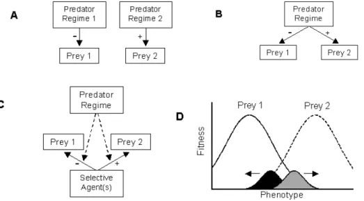
A central goal of evolutionary ecology is to understand the roles of different ecological processes in producing patterns of evolutionary diversification. Theoretical and empirical studies have shown that competition and antagonistic interactions such as prey/predator or host/parasite interaction can promote diversification or maintain biological diversity (see chapter I.3 p.37).
Concepts and Background
The potential of a population to adapt to an environment depends on its genetic variance [3]. In this context, determining the distribution of the genetic variance of a population and the factors contributing at the origin, as well as the maintenance and distribution of this genetic variance observed remain central and fundamental research issues [4]. Population genetic variation arises through random mutations. According to natural selection theory, environment influences the evolution of populations by selecting the best adapted individuals. Natural selection and therefore many factors like competition for resources, spatial structure, biotic factors (e.g., predation, parasitism) influence which individuals will survive and reproduce. The tendency of alleles to spread over time in a population is then due to survival and reproductive success.
Genetic drift is a random process occurring at each generation, involving random variations in the number of offspring [5]. According to the neutral theory of molecular evolution, some alleles arising by mutation fluctuate in frequency according to the – random – number of offspring of their carriers. In the long run, this process leads to the eventual loss or fixation of mutations in the population. The most persuasive argument in favor of the neutral theory is that the less functionally important one genome area is the more variable it is. It is thus important to determine the relative contributions of neutral and selective factors in influencing genetic variability.
1.1 Neutral polymorphism
Based largely on a brilliant series of papers by Kimura in the 1960s and 70s and by King & Jukes 1969 [6], the neutral model of evolution has become the standard by which positive selection must be separated from genetic observations. In the neutral theory, the vast majority of mutations are subdivided into two groups. The first group, after which the model is named, is selectively neutral (or effectively neutral) mutations which eventually become lost or fixed in a species by genetic drift. The later substitutions account for almost all the observable nucleotide changes between two species. The second group is selectively deleterious mutations, which may frequently arise continuously and are eliminated over time by natural selection. Because these mutations are eventually and generally eliminated from a species, they are rarely observed when comparing the genomes of two species. The vast majority is counter-‐selected or neutral. Only a small fraction of them are positively selected. Because they cause mutant phenotypes, these mutations are well known to functional geneticists, since they account for nearly all of the mutant strains and human diseases that are much studied throughout biology and medical research.
1.2 Demography and genetic drift
Stochastic variations in the environment lead to fluctuations in population size. The influence of such stochastic variation is proportionally greater for small populations than for large ones. The smaller the population the greater the probability that fluctuation will eventually lead to extinction is. They are subject to a higher chance of extinction and are more subjected to genetic drift, resulting in stochastic variation of their gene pool. Genetic variation is determined by the joint action of natural selection and genetic drift (chance). The relative importance of genetic drift in a small population is higher, since any allele, deleterious, beneficial or neutral is more likely to be lost or fixed.
1.3 Natural selection, biotic factors and spatial structure 1.3.1 Natural selection
Selection occurs when one genotype leaves on average a different number of progeny that of another. This may happen because of differences in survival, in mating or in fertility.
Positive selection is the process by which new advantageous genetic variants invade a population. Positive selection, also known as Darwinian selection, is the main mechanism that Darwin envisioned as being responsible for phenotypic evolution.
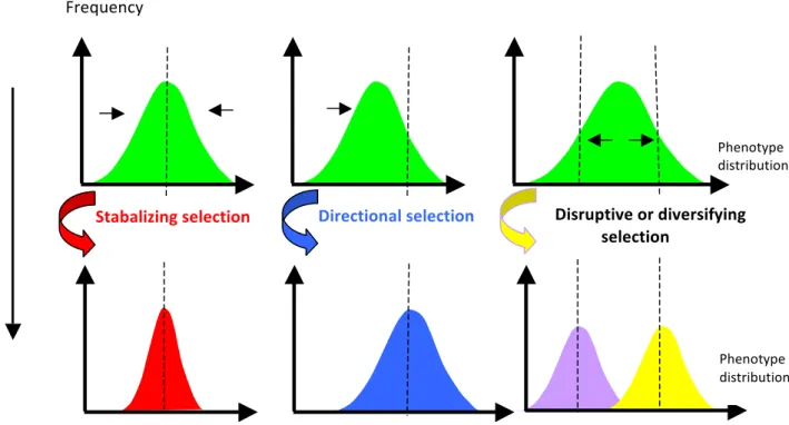
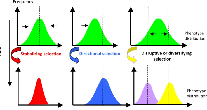
There are three general selection regimes (Figure I-‐1):
Directional selection occurs when selection favors one extreme phenotypic trait value over the other extreme. This typically results in a change in the mean value of the trait under selection.
Disruptive selection occurs when selection favors the extreme phenotypic trait values over the intermediate trait values. In this case, the variance increases as the population tends to be divided into two distinct groups.
Stabilizing selection occurs when selection favors the intermediate phenotypic trait value over the extreme values. Populations under this type of selection typically experience a decrease in the amount of additive genetic variation for the trait under selection.
Figure I-1: The three basic selection regime
Dotted traits indicate the optimum expressions of the phenotype. Horizontal arrows show the directions of selective forces.
Phenotype distribution
Stabalizing selection Directional selection Disruptive or diversifying selection Phenotype distribution Frequency Ti m e
1.3.2 Biotic factors
Biological interactions result from the fact that organisms in an ecosystem interact with each other in the natural world, since no organism is an autonomous entity isolated from its surroundings, but it forms part of its environment. Ecological interactions such as competition and antagonistic interactions play a central role in diversification.
There is mounting evidence that natural selection and in particular balancing selection, has played a major role in many evolutionary diversifications and/or in maintaining polymorphism. By balancing selection, population geneticists mean any form of selection that promotes polymorphism, for example by overdominance (heterozygote superiority in fitness) or frequency-‐dependent selection (FDS), which favors different genotypes in different environments [7] (see Chapter I.3, p.37).
1.3.3 Spatial structure
Nature is definitely spatially structured. First, individuals interact preferentially with individuals in their neighborhood (populations are not homogeneous). Secondly, connections between individuals are often correlated with spatial proximity (geographical distance). Spatial structure is likely to have important evolutionary consequences in natural selection. Such effects on evolution and adaptation have been widely studied using theoretical models (see e.g. [8, 9]).
In asexual organisms, adaptation proceeds more slowly in a spatially structured environment than in one where competition is global [10]. An important phenomenon that limits adaptation in asexual is the Hill–Robertson effect [11], which is. clonal interference among advantageous haplotypes [12]. In asexual organisms, clones with different beneficial mutations compete with each other, only one becoming fixed in the population.
1.4 Selective sweep
Natural selection is the driving force for the phenotypic adaptation of organisms to a changing environment. Selective pressure applied to individuals leads to changes in the genetic content of the population. Organisms bearing a more adapted genotype would outcompete their peers. It results in the fixation of beneficial allele(s) in the population. Genes that are subject to selection are usually
found in the context of a chromosome. Adjacent genomic segments physically linked to the selected genes are therefore either dragged to fixation along with the beneficial allele or discarded with the less fit alleles during the process called genetic hitchhiking. The strength of hitchhiking decreases with the genetic distance from the selected locus and recombination can eventually separate the selected allele from adjacent loci (Figure I‐2). Figure I‐2: Selective sweep/Hich‐hiking (a) The neutral mutation physically linked to the advantageous mutation will be fixed. (b) The strength of hichhiking decreases with the distance from the selected locus. Hich‐hiking leads to a local decrease of diversity. [13] The processes of natural selection and genetic drift are complex. Our approach was to combine experimental evolution and modeling to disentangle the effect on neutral polymorphism of these evolutionary forces. 2.EXPERIMENTAL EVOLUTION AND MODELING 2.1 Experimental evolution In evolutionary and experimental biology, the field of experimental evolution is concerned with testing hypotheses and theories of evolution by use of controlled experiments. Evolution may be observed in the laboratory as populations adapt to new environmental conditions and/or change by such stochastic processes as random genetic drift.
(a)
2.1.1 Early experimental evolution
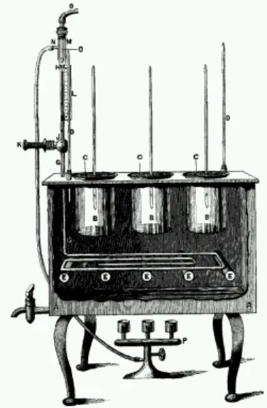
One of the first to carry out a controlled evolution experiment was William Dallinger., who cultivated small unicellular organisms in a custom-‐built incubator (Figure I-‐3) over period of six years during the late 19th century (1880-‐1886) [14].
Figure I-3: Drawing of the incubator used by Dallinger in his controlled evolution experiment
The President's Address. J. Royal Microscop. Soc., pp. 185-‐199, 1887. (Actual image is Fig. 31 on page 193).
Dallinger slowly increased the temperature of the incubator from an initial 15.5°C to 70°C. The early cultures had shown clear signs of distress at a temperature of 22.7°C, and were certainly not capable of surviving at 70°C. on the other hand, the organisms Dallinger had in his incubator at the end of the experiment were perfectly fine at 70°C. However, these organisms would no longer grow at the initial 15.5°C. Dallinger concluded that he had found evidence for Darwinian adaptation in his incubator, and that the organisms had adapted to live in a high-‐temperature environment. Unfortunately, Dallinger's incubator was accidentally destroyed in 1886, and Dallinger could not continue this line of research.
2.1.2 Modern experimental evolution
From the 1880s to 1980, experimental evolution was intermittently practiced by a variety of evolutionary biologists, including the highly influential Theodosius
Dobzhansky. Like other experimental research in evolutionary biology during this period, much of this work lacked extensive replication and was carried out only for relatively short periods of evolutionary time. But by 1980, a variety of evolutionary biologists realized that the key to successful experimentation lay in extensive parallel replication of evolving lineages as well as in using a greater number of generations of selection. One of the first of a new wave of experiments using this strategy was laboratory "evolutionary radiation" of Drosophila melanogaster populations that Michael R. Rose started in February, 1980. This system began with ten populations, five of which were cultured at older ages, and five at early ages. Since then more than 200 different populations have been created using laboratory radiation, with selection targeting multiple characteristics. Some of these highly differentiated populations have also been selected "backward" or "in reverse," by returning experimental populations to their ancestral culture regime. Hundreds of people have worked with these populations over the last three decades.
More recently, many groups carried out evolution experiments using diverse organisms including plants, vertebrates and in particular microorganisms. Many microbiologists realized that microbes offer powerful systems for evolutionary insights. (Box 1).
Box 1:| Advantages of microorganisms for evolution experiments
Microorganisms that have been used in experimental evolution include many bacteria and viruses, as well as unicellular algae and fungi. These organisms are well suited for such experiments for many practical reasons:
-‐ They are easy to propagated.
-‐ They reproduce quickly, which allows experiments to run for many generations. -‐ They allow large populations in small spaces, which facilitate experimental replication. -‐ They can be stored (i.e. frozen) in suspended animation and later revived which allow direct comparison of ancestral and evolved types.
-‐ Many microbes reproduce asexually and the resulting clonality enhances the precision of experimental replication.
-‐ Asexuality also maintains linkage between a genetic marker and the genomic background thus facilitating fitness measurements (Box 2 p.23).
-‐ It is easy to manipulate environmental variables, such as resources, as well as the genetic composition of founding populations.
-‐ There are abundant molecular and genomic data for many species, as well as biotechnological tools for their precise genetic analysis and manipulation.
Importantly, adaptation can be quantified by measuring changes in fitness in the experimental environment, in which fitness reflects the propensity to leave descendants [16, 17].
Fitness can be measured by competition between an evolutionary line and its genetically marked ancestor (Box 2).
Box 2: | Measuring fitness
[15] Measuring Fitness:
Relative fitness W is calculated as the ratio of the growth rate of one strain relative that of another during their direct competition. Nevertheless, it is preferable to express performance in terms of selection rates, r (see below) (i)
when one competitor is much less fit than the other [18] or (ii) when one or both
competitors are declining in abundance, such as during competitions assays under starvation conditions or in the presence of an antibiotic (Box3).
Box 3: | Example of W and r calculation
Two strains A and B are growing up separately proliferating to a density of ~4.109
cells/ml. At time 0 of the competition experiment, the density of each strain is adjusted to 2.107 cells/ml. After an appropriate dilution (two successive 100 fold factors) and plating
of 0.1 ml; a sample yields 192 colonies of A and 204 colonies of B. At time 0:
A(0)= estimated density of A at time 0 A(0)= 192x10x100x100 = 1.92.107 cells/ml
B(0)= estimated density of B at time 0 B(0)= 204x10x100x100
B(0)= 2.04.107 cells/ml
The mixed population grows and competes over one day. At the end of which the total density has grown back to 4.109 cells/ml. After an appropriate dilution (three successive
100 fold factors) and plating of 0.1 ml, a sample yields 319 colonies of A and 107 colonies of B.
At time 1:
A(1)= estimated density of A at time 1 day A(1)= 319x10x100x100x100
A(1)= 3.19.109 cells/ml
B(1)= estimated density of B at time 1 day B(1)= 107x10x100x100x100
B(1)= 1.07.109 cells/ml
To estimate the relative fitness W, we can define mA and mB, as the realized Malthusian
parameters respectively for strains A and B:
mA= ln[A(1)/A(0)]/day
mB=ln[B(1)/B(0)]/day
The relative (Darwinian) fitness W is the ratio of the Malthusian parameter:
W= mA/mB = 1.29
During the competition, A increased about 29% faster than B.
The selection rate is equal to the difference between the two strains’Malthusian parameter during direct competition.
Hence the estimation of the selection rate, r is:
r= (ln[A(1)/A(0)]-‐ln[B(1)/B(0)])/day r= 1.153 per day.
Over the course of one day of competition, the density of A increased by around 1.1 natural-‐logs more than the density of B did.
Many microbial evolution experiments were begun to explore the interesting dynamics that can emerge from complex interactions among several components of a larger system. There is a growing interest in evolution experiments that are carried out in silico.
2.2 Modeling biology 2.2.1 Modeling
Given the complexity of both ecological and evolutionary processes, it is necessary to make several simplifying assumptions in the development of theories. Modeling is an approach to assess complex natural phenomena using simplified assumptions in the development of theories.
2.2.2 Population genetics models
Mathematical population genetics addresses the question about gene frequency distributions in analytical form. Fisher, Haldane and Wright [3, 19, 20] together shaped the foundations of the field and are referred to as the ‘great trinity’ of population genetics. In particular they produced seminal papers in this field.
A primary focus of mathematical population genetics concerns fixation probabilities, which is the probability that a given allele in a population will ultimately invade the whole population. Empirically, fixation probabilities can be related to the rate at which a population adapts to a changing environment, the rate of loss genetic diversity or the rate of emergence of drug resistance. Analytical results may be derived under simple conditions to which more complex cases assessed through simulations should be compared.
There are three approaches to computing fixation probabilities.
When the population size is quite small, the state space of a population (exactly how many individuals have exactly which genotype) can be enumerated, using a markov chain approach to exactly determine the fixation probability (see Gale
1990 ) [21].
When the population size is large, methods based on discrete branching processes are often used. These methods build on the ‘Haldane–Fisher’ model [3, 19], and can be related to a Galton–Watson branching process. It provides an approximation to the true fixation probability, since it assumes that the wild type population is sufficiently large for the fate of each mutant allele to be independent of all the others [22-‐26].
Finally, when the population is large and the change in allele frequency per generation is small in each generation (i.e. weak selection), methods that incorporate a diffusion approximation may be used.
Haldane [19] showed that the probability of ultimate fixation, π, of an advantageous allele with selection coefficient s is π =2s when the allele is initially present as a single copy in a large and constant population size (and s is not too large). Other assumptions include discrete generations and a Poisson distribution of the number of offspring.
Kimura’s approach was to use a diffusion approximation model. The main result is that the probability of ultimate fixation π of an allele with an initial frequency p is:
(1)
Where Ne is the effective population size (the equivalent size of an ‘ideal’
population).
When p=1/2Ne, this probability of fixation tends to the previous result 2s.
The same expression was obtained by Moran (1960) and Gillespie (1974) [27] using slightly different approaches.
Population of variable size:
-‐ Growing and declining or cyclic population sizes
Ewens (1967) [28] used a discrete multiple branching process to study the
survival probability of new mutants in a population that assumes cyclic sequence of population sizes that matches a typical experimental set up. Ewens derived corresponding ultimate probability of an initially unique mutant:
(2)
where Ñ
is the harmonic mean and is the arithmetic mean of the population
sizes in the cycle.
Ewens found that the π value may be considerably less than 2s, implying that a constant population size is favorable for the survival of new advantageous mutants whereas fluctuations slow adaptation.
Otto and Whitlock (1997) [22] later built on the work of Ewens and Kimura in populations modeled by exponential and logistic growth or decline.
Pollak (2000) [29] studied the fixation probability of beneficial mutations in a population changing cyclically in size and proved that the result found for Poisson-‐
distributed offsprings by Ewens (1967) [28] and Otto and Whitlock (1997) [22] still holds in situations where the Poisson offspring distribution is not necessary.
-‐ Population Bottlenecks
A population bottleneck is a sudden, severe reduction in population size with subsequent recovery of greater population size. An important assumption to note is that after the population bottleneck, each individual—mutant or wild-‐type—is assumed to survive the bottleneck with the same probability. Thus the ‘offspring’ distribution of each individual at the bottleneck is the same, for either mutant or wild type, i.e., no selection occurs. In contrast, during growth any selective advantage for the mutant can be achieved.
Wahl & Gerrish (2001) [23] derived the probability that a beneficial mutation is
lost due to population bottlenecks using both a branching process approach [3, 19] and a diffusion approximation [30-‐32]. When selection is weak, the two approaches provide the same approximation for the extinction probability X
(X=1-‐π) of a beneficial mutation that occurs at time t between bottlenecks:
(3)
where s is the selective advantage of the mutant over the wild type strain, r is the Malthusian growth rate of the wild type population and τ is the time at which a bottleneck is applied. It was thus found that the fixation probability,π , drops rapidly as t increases, implying that mutations that occur late in the growth phase are unlikely to survive population bottlenecks, they have not enough time to increase in frequency and survive bottleneck.
Experimental techniques in microbial evolution have advanced to the point where the fate of a new mutant strain within a controlled population can be tracked over many generations.
2.3 Experimental evolution and modeling
Several experiments have provided some of the most relevant data for testing predictions about such branching points [33-‐35]. Most of them have been conducted using microbial cultures, such as Pseudomonas or Escherichia coli. Such model organisms are ideal for testing this theory because their short generation
times and well-‐defined genetic stocks make evolutionary experiments feasible. For example in single strain of E. coli propagating in glucose medium, evolutionary diversification eventually took place, resulting in the stable maintenance of two distinct physiological types [33, 36]. Similarly, in colonies of a single strain of Pseudomonas propagated on a complex liquid medium, evolutionary diversification eventually took place, resulting in three well-‐defined types that appear to coexist indefinitely (the “fuzzy spreader”, “wrinkly spreader” and “smooth” types; see [37]). These morphs appear to exploit spatial niches in the liquid medium.
Conclusion
In the absence of information concerning the selective regime, most simple models are classically used to study such processes: constant coefficient of selection across time, space, no frequency dependence, absence of interference between selective events, no interaction with demography. Natural conditions probably largely violate these assumptions, and the issue is then to assess the corresponding effect on genetic variability.
The occurrence of genetic drift is difficult to demonstrate in natura and to distinguish from selective effects. It is also difficult to test experimentally, because of the long time scales involved. Moreover, the results of evolutionary experiments are generally interpreted without taking into account stochastic processes and are often confounded with experimental error. Nevertheless, these stochastic phenomena can sometimes be the sole explanation for an observation. There is therefore relatively little data available on genetic drift (see however Buri 1956 [38]).
To study these evolutionary forces, the most direct approach, used here, relies on the analysis of temporal variations of allele frequencies [39]. However, one of the issues addressed in this thesis is to what extent such frequency variations are due to random phenomena, or to selective effects. Genetic drift leads to frequency fluctuations than can go either way thus allowing disentangling it from selection which typically is unidirectional. When an advantageous mutation appears in a genome, provided it escapes initial loss by drift, it tends to increase in frequency and eventually reaches fixation, thereby replacing pre-‐existing variation on the target locus. Furthermore, the genomic area in which it appeared is then swept of neutral mutations, which otherwise accumulate within non-‐functional DNA. This phenomenon, called selective sweep or hitchhiking, provides a powerful tool to detect rare selective events through their effect on the neighboring neutral loci [40]. During our experiments, the selective regime will be provided by a biotic factor of prey-‐predator type. In prey-‐predator interactions, environments often change quickly, and therefore impose a fluctuating selective pressure on its prey unlike the traditional assumptions of population genetics models. Similarly, the predator population should strongly affect the prey demography and vice versa.
The choice of the biological model is then primordial to perform evolution experiments. Such ecological factors will be included in the population genetics models. Since the influence of selection and genetic drift processes on diversity is complex, a relevant model is needed in order to provide quantitative predictions to be tested on the corresponding experimental data.