HAL Id: hal-00932195
https://hal.inria.fr/hal-00932195v2
Submitted on 4 Nov 2014
HAL is a multi-disciplinary open access
archive for the deposit and dissemination of sci-entific research documents, whether they are pub-lished or not. The documents may come from teaching and research institutions in France or abroad, or from public or private research centers.
L’archive ouverte pluridisciplinaire HAL, est destinée au dépôt et à la diffusion de documents scientifiques de niveau recherche, publiés ou non, émanant des établissements d’enseignement et de recherche français ou étrangers, des laboratoires publics ou privés.
Fast Construction of Efficient Structured Peer-to-Peer
Overlays
Lokman Rahmani
To cite this version:
Lokman Rahmani. Fast Construction of Efficient Structured Peer-to-Peer Overlays. Distributed, Parallel, and Cluster Computing [cs.DC]. 2013. �hal-00932195v2�
Polytech’Nice Sohpia
Stage de Fin d’Etudes
[R]
Université de Nice Sophia-Antipolis
2013
INRIA Sophia Antipolis - Méditerranée
Fast Construction of Efficient Structured
Peer-to-Peer Overlays
Student: Lokman RAHMANI
[email protected] - Master 2 IFI - CSSR
Supervisor : Fabrice HUET
[email protected] - INRIA - OASIS Team
Academic tutor : Arnaud LEGOUT
Contents
1 Introduction 6
1.1 What is a DHT?[23] . . . 6
1.2 Applications on top of DHTs . . . 8
1.3 Contributions . . . 8
1.3.1 Model for Building Efficient DHTs . . . 9
1.3.2 Load- and traffic-balancing . . . 9
1.3.3 Data Transfers Minimization . . . 10
1.4 Organization . . . 11
2 Preliminaries 12 2.1 Reference Definition of Structured Overlay Networks[6]. . . 12
2.1.1 The virtual identifier space . . . 12
2.1.2 Mapping peers to the identifier space. . . 13
2.1.3 Mapping resources to the identifier space . . . 13
2.1.4 Management of the identifier space . . . 13
2.1.5 Graph embedding . . . 14
2.2 CAN : Content-Addressable Networks . . . 15
3 Model for Building Efficient DHTs 17 3.1 Philosophy . . . 17
3.2 Load-balancing . . . 17
3.3 Traffic-balancing . . . 18
3.4 General model for optimal join . . . 19
4 Load- and Traffic-balancing 21 4.1 Managing the DHT. . . 21
4.2 Skip List as a Distributed Structure . . . 22
4.3 Experimental Evaluation. . . 24
4.3.1 Experiments setup . . . 24
4.3.2 Results & Discussion . . . 24
5 Data Transfers Minimization 25 5.1 Understanding Data transfers . . . 25
5.2 Incoming Data Transfers Minimization . . . 27
5.3 Outgoing Data Transfers Minimization. . . 27
5.3.1 Building partial view . . . 27
5.3.2 Take Decision based on partial information . . . 29
5.3.3 Heuristic for outgoing data transfers minimization (ODMH) . . . 30
5.4 Experimental Evaluation. . . 34
5.4.1 Experiments setup . . . 34
5.4.2 Results & Discussion . . . 34
6 Conclusion 38
.
ABSTRACT
This report presents algorithms for building Distributed Hash Tables (DHT) or Structured Overlays. DHTs are used as self-managing system to handle distributed data in large networks. Our algorithms ca be used to build efficient DHTs with several properties or to recover fastly the last configuaration of a DHT after crash or exit.
In DHTs, the managed data distribution can be non uniform, and if we build the DHT using canonical algorithms it will create load imbalance between participating machines (or peers): it will take a lot of time and will lead to a DHT with poor performances. So to ensure efficiency in the general case, we first introduce a general easy-to-use model that can be used to consider several properties, that guarantee DHT performances. Based on that model, as a practical solution, we provide a distributed structure that permit to reorganize the DHT to facilitate the join of new machines, while considering the selected properties. As an example, this structure was used to ensure both load- and traffic-balancing over DHT machines.
To fast build DHTs, we need to have a global knowledge about DHT status, as we need to consider some properties related to the new peers characterstics. Nevertheless DHTs are distributed structures, i.e. each participating peer maintains a local state of the DHT which includes itself and a small number of its neighbors. No one peer have a global view of the whole DHT. To overcome this obstacle, we provide an algorithm that build a partial view of the DHT more interesting than the local one. Based on this partial view, we develop a heuristic that minimize data transfers by considering the input data of each new peer. This reduces clearly the time to build an operational DHT.
All the algorithms we will present have been implemented and tested using simulation. We will talk briefly about the simulation tools and environment. We will also present and discuss our experimental results.
.
ACKNOWLEDGEMENTS
I truly feel privileged to have worked under the supervision of Dr. Fabrice Huet. He introduced me in the research area of distributed systems. He was available all the time and provide me advises and knowledge on both the theoretical and practical work. I would like also to thank all OASIS team members for their hospitality and rich discussions during my internship. In particular, I thank Amjad Alshabani, Iyad Alshabani, Laurent Pellegrino and Maeva Antoine. I would like to show my gratitude to Dr. Arnaud Legout who accepts to read and comment my reports. Finally, I would like to acknowledge all the academic team at Polytech’Nice Sophia and University of Nice Sophia-Antipolis that manages the IFI master and make it richer and more interesting.
1
Introduction
Nowadays applications generate, consume and process a large amount of data. This make the need to provide platforms and systems that can deal with this huge load of data.
Distributed hash tables (DHTs) are very used to manage distributed data in an efficient manner. In a network with many machines, Data objects can be stored and retrieved in short time from any machine of the network.
The aim of this chapter is to introduce the topic. First we will talk about DHTs, their advantages, and some of their applications. After we will present our contributions on building efficient DHTs and compare them to the related work. Finally the organization of the report is presented.
1.1
What is a DHT?[
23
]
A distributed hash table is, as its name suggests, a hash table which is distributed among a set of cooperating computers, which we refer to as peers. Just like a hash table, it contains key/value pair. The main service provided by a DHT is the lookup operation, which returns the value associated with any given key. In the typical usage scenario, a client has a key for which it wishes to find the associated value. Thereby, the client provides the key to any one of the nodes, which then performs the lookup operation and returns the value associated with the provided key. Similarly, a DHT also has operations for managing items, such as inserting and deleting data items.
The representation of the key/value pairs can be arbitrary. For example, the key can be a string or an object. Similarly, the value can be a string, a number, or some binary representation of an arbitrary object. The actual representation will depend on the particular application.
An important property of DHTs is that they can efficiently handle large amounts of data items. Because of limited storage/memory capacity and the cost of inserting and updating items, it is infeasible for each node to locally store every item. Therefore, each node is responsible for part of the data items, which it stores locally.
As we mentioned, every node should be able to lookup the value associated with any key. Since all items are not stored at every node, requests are routed whenever a node receives a request that it is not responsible for. For this purpose, each node has a routing table that contains pointers to other nodes, known as the node’s neighbors. Hence, a query is routed through the neighbors such that it eventually reaches the node responsible for the provided key.
Consistent Hashing - A hash table uses a hash function applied to keys to get an index where
to store associated data items. Just like hash table, the DHT also uses a hash function to decide in which peer a key/value item will be stored. The difference is that the hash function maps keys to a
pre-defined virtual space (e.g. 2-Dimensional Cartesian space) which is more general than integer indexes. An addition is that also peers will have identifiers from the same virtual space. Then, each peer will be responsible on keys/values items that are close to its identifier considering some defined metric. This is what is called consistent hashing. Consistent hashing was introduced in the context of web pages caching on multiple node in the Internet[29,19]. To ensure load balance over peers, the hash function is supposed to be uniform: the stored keys/values items are uniformly distributed over the virtual space, such that each peer will store approximatively the same amount of data items.
Range Queries - In some applications, it might be useful to ask the DHT to find values associated
to all keys in a numerical or an alphabetical range. For example, in a grid computing environment, the keys in a DHT can represent CPU power. Hence an application might query the DHT to search for all key in the interval 2000-4000 MHz. DHTs does not support naturally ranges queries. Over the last years, many works have been done to consider range queries [11,15,33, 25]. The Play project used the solution proposed by A. Datta and al. in [21]: the use of order-preserving hash function to map keys to the virtual space. Formally an order-preserving hash function hop is a function that ensures if we have
two keys k1, k2 and k1 < k2 then we have hop(k1) <v hop(k2), where < and <v are ordering relation
defined in the keys space and virtual space respectively. From this definition a uniform hash function is clearly not an order-preserving hash function. So When using such hash functions this will lead to load-imbalance over peers. In this report we present algorithms that ensure load-balance and can ensure multiple criteria even when using order-preserving or non-uniform hash function in general.
Building DHTs - DHTs are built incrementally. The first peer will manage all DHT data. As well
as new peer arrives and join the DHT, it becomes responsible of a part of DHT data that it get from a unique DHT peer. This peer is called the join peer.
For a new peer to know about the DHT and select the join peer, most of DHTs make use of a directory that maintains a list of peers that are participating to the DHT. So a new peer will first contact the directory to get a random DHT peer, called entry peer. The new peer calculate then its identifier (based on information about the DHT that it get from the directory or the entry peer) and ask the entry peer to find the DHT peer with identifier that is closest to its identifier. Once found, the insertion is done with the participation of the new peer, the join peer and its neighbors.
Structured Overlay networks - DHT is said to construct an overlay network because its peers
are connected to each other by links established at the application layer and are completely different from physical links that connect machines hosting peers. Figure1.1ilustrate an overlay network and the physical network it relays on. DHTs are classified as structured overlay networks as the links forming the overlay are established between peers in a way to form a specific topology (a ring, tree, ...).
Figure 1.1: An overlay network built at the application level and the physical network it relays on.
As we will talk only about structured overlays, for simplicity we will omit the word ’structured’ in structured overlays.
1.2
Applications on top of DHTs
We have described what is a DHT and some of its concepts, in this section we talk very briefly about some applications that use DHTs. In almost all cases, DHTs are not used as is, but serves as a lower layer to manage data of different distributed system as we will see.
Publish/Subscribe systems - In a Publish/Subscribe system there are two types of roles, as its
name suggests : publisher and subscriber. Publishers are those who generate and provide contents. Subscribers are content consumers. A subscriber present its interest to a part of content by making subscriptions to the topics he want to receive content about. The role of a Publish/Subscribe system is to save all subscriptions, and when receiving content on a topic, forward it to all subscribers for that topic.
It’s clear that with the presence of many publishers and many subscribers that the system will have a huge load of content to receive, store and deliver at real-time. This becomes more difficult when pub-lishers and subscribers are geographically distributed. This is the aim of the Play[5] European project to build a Publish/Subscribe system that covers most of Europe. OASIS team; as a responsible of data management part; adapted a DHT-based storage system [34]. Many other works have been done on using DHTs in Publish/Subscribe systems like [37]. Our work is in that context to build efficient DHT-Based storage considering several properties.
Cloud Key/Value Storage - Very recent usage of DHT-Based storage is their adaptation in the
context of Cloud Computing. In the Cloud model/philosophy, companies (like Google, Amazon) provide solutions and applications for their clients transparently and can be used virtually from anywhere with a very high availability, where all computation and data management is done in the server side, the client side have to provide resources only for the visualization.
To ensure that, big companies deploy all over the world many powerful data-centers. In this case the big deal is to ensure high-availability where the systems receive accesses and queries from thousands of clients from all the world. To meet this requirements, many DHT-based storage systems have been proposed and deployed, augmented by some additional properties (like consistency, availability, parti-tion tolerance) and are known as key/value storage [22,13,20]. Our work can be also used well in that context.
Other uses of DHTs - DHTs have been used in many other contexts. we can cite :
• Host discovery and mobility: like Internet Indirection Infrastructure (i3) [38], Host Identity Payload (HIP)[4], ...
• Web caching and web servers: Squirrel[26], DKS Organized Hosting (DOH)[28]
• In peer-to-peer file sharing applications : BitTorrent[16], Azureus, eMule, and eDonkey use the Kademlia DHT[31].
1.3
Contributions
Our work is principally about building DHTs. This section resumes our contributions and compare them to related work. Later, each contribution is described more in details, and main results are presented and discussed; each contribution in separate chapter.
1.3.1 Model for Building Efficient DHTs
To build rapidly efficient DHTs we need to ensure several properties at the same time. Based on a reference definition of DHTs[6], we provide a model to build efficient DHTs in reasonable time ensuring selected properties. We modeled this problem as an ILP1 problem. Each property to ensure is called
criterion. Each criterion is associated a cost. All selected criteria are grouped in an objective function
that we want to optimize (minimize or maximize).
When a new peer want to join the DHT, it has to find the best peer to be inserted so that it optimizes the objective function and then satisfy most of the criteria. In this model we distinguish two types of criteria: intra-DHT criteria and extra-DHT criteria. Intra-DHT criteria can be calculated based only on the DHT state like load-balancing and traffic-balancing, and thus are independent from the new peer that want to join the DHT. In the other side an extra-DHT criterion depends also on the new peer and its evaluation changes for each new peer. An example of an extra-DHT criterion is data transfer minimization where the quantity of data transfers will depends on the new peer input data.
An important point to note, is that this model can’t be used directly as it supposes the availability of a global view of the DHT status, so that we can calculate all possible solutions to the ILP. But it serves as a reference to the optional solution we can get. All other contributions are based on that model. We will see after for the two next contributions how can we overtake this obstacle by managing the DHT to consider intra-DHT criteria or by building a partial view sufficient enough to get the optimal solution in short time or at least a good solution for a specific extra-DHT criteria.
Related Work - We are not aware of any related work at the general level, or any work that address
new peers insertion while ensuring multiple properties. For fast building DHTs, many works have been done on the parallelization of new peers join to do parallel joins starting from a specific topology that connects the peers before deciding to bootstrap the DHT[12,17]. Clearly those algorithms don’t address the efficiency of the built DHT and also don’t lead to operational DHT in the case where peers have their input data. Also those works can be used only in the bootstrap phase and don’t consider future new peers joins.
1.3.2 Load- and traffic-balancing
We propose the use of a distributed structure based on a skip list[35] so that it will manage the DHT to facilitate access to the join peer [that satisfies the most of efficiency properties]/[to have efficiency]. The Skip list can be seen as practical solution to the model to consider criteria that depends only on the DHT status (intra-DHT criteria).
As a demo the skip list has been used to ensure both load- and traffic-balancing while building the DHT. Load-balancing ensure that the quantity of data each peer have to manage is approximatively the same for all peers. Traffic-Balancing consider the number of messages each peer receive or forward, while new peers are joining the DHT or users are querying for data items. Those two criteria have an important impact on the DHT efficiency.
Related Work - Lots of work have been done to ensure load-balancing and traffic-balancing that
we don’t want to detail here. Very briefly, to ensure load-balancing, almost all solutions fold in two categories. In the first category over-loaded peers have to find underloaded ones to send to them some of their load. The main difference with our solution is that we address the problem in the building phase while those solutions address it after when using the DHT. So we can consider that our solution and others are complementary. Also we don’t transfer data to ensure load-balancing we just take profit from the mandatory transfers when the status of the DHT changes. The other category introduce the notion
of virtual peers. The idea behind is instead of moving data directly between peers, if a peer detect that it is overloaded it creates a new peer; the virtual peer; that will be responsible for a part of its data and will be hosted on the machine where an underloaded peer is running. for those solutions our work can be well used even when the building is terminated as the creation of virtual peer is considered as a regular peer join operation.
A closest work to our was proposed by H. V. Jagadish and Al. in [27], where they use a tree-based overlay augmented by a skip list to redirect the new peers to the overloaded peers. This work was applied only on specific DHT (BATON) and consider only one property (load-balancing) where our solution is general can consider several properties based on the model we first define.
1.3.3 Data Transfers Minimization
When building DHTs, each new peer insertion induce uncontrollable data transfers due to the changing of the configuration of the DHT and the input data of new peer that it want to store in the DHT. Minimizing those transfers is important to fast build operational DHTs: DHTs that are ready to use and all data stored in is accessible for users.
Following the model we introduced in contribution 1.3.1, data transfer minimization is an extra-DHT criterion. In fact, it depends on the input data of each peer.
So following the construction procedure, a new peer will look for the join peer from the DHT that will induce less transfers considering its input data. This will need a global knowledge that doesn’t exist, unless it contacts all DHT peers which is too costly. Considereing that we introduce an algorithm that build a partial view that is more intersting than the local one. After that we exploit this partial view to develop a heuristic that minimize new peers data transfers after joining the DHT. The heuristic in the best case find the the optimal join peer to insert the new one, and in the worst case have a very low overhead. We also provide and discuss our experimental results.
Related Work - In our best knowledge no work has been done on data transfer minimization when
building DHTs. But many related work have been done to consider some criteria that are close to our as
content-Locality and network-locality. Content-locality [1,40,24] ensure that each peer will store locally its input data. This was proposed mainly for data confidentiality issues as well as path-locality[24]. Content-locality is a criteria that is stronger than data transfer minimization in case where if each peer keeps its input data there will be no transfers. Unfortunately the resulted overlay is not a DHT but just an indexing overlays. So those works can’t be adapted to our criteria in the context of Building DHTs. Also those solutions don’t deal with efficiency issues like load-balancing.
An other criteria that is similar to our, in the way that is also an extra-DHT criterion (i.e it depends on both DHT status and new peer characteristics) is Network-locality[8,41,18,30]. Ensuring network-locality requires that the build DHT neighborhoods will approximatively reflect the physical network links, in the goal to reduce latencies of messages exchanged between neighbor’s peers. This imply for each new peer, at the building phase, to find the join peer that is physically close to it among all DHT peers. The criterion of network-locality is well studied. Some proposed solutions based on groups are mainly centralized[41]. Other need a heavy maintenances of the groups[30]. There is also very efficient and distributed solutions[18], but unfortunately are problem-specific, and relay on the hierarchy pf IP addresses to define proximity classes. An other point that make data transfer minimization more challenging is that data changes over time which is not the case for IP addresses that are fixed for each peer. Other differences that make hard the adaptation of solution proposed for network-locality are discussed in details in [3].
1.4
Organization
The chapters of this report are organized as follows :
• Chapter 2 provide a general reference definition of DHTs that we will base on to develop our algorithms. It also presents Content-Addressable-Networks (CAN) as an example of DHTs that we will refer to, all over this report. Finally the chapter presents the canonical algorithm used to build DHTs.
• Chapter 3 Describe the proposed model to build efficient DHTs in the general case. This is done by considering several properties to ensure, to have performances.
• Chapter 4 Based on the model described in the previous chapter, this chapter presents a practical solution that uses a distributed structure (a Skip List) to manage the DHT in a way to facilitate the join of new peers while ensuring properties related to the DHT. This structure was used, as a demonstration, to ensure Load- and traffic-balancing together.
• Chapter 5 shows how can we build a partial view of the DHT, that is more interesting than the local one, knowing that the DHT is a distributed structure over participating peers. the chapter also presents how can we exploit the partial view to minimize data transfers when building the DHT.
2
Preliminaries
This chapter present a reference definition of structured overlays (and thus DHTs included) that we will base on to develop our algorithms. It also describes briefly Content-Addressable-Networks or CAN as the example of DHTs that we will refer allover this report for giving examples or for practical evaluations. Finally the chapter explain again how to build DHTs referring to the presented definition of overlays.
2.1
Reference Definition of Structured Overlay Networks[
6
]
In any overlay a group of peer P provides access to a set of resources R (data items in our case) to an (application-specific) virtual identifier space I using two functions : FP : P −→ I and
FR : R −→ I . These mapping establish an association of resources to peers using a closeness metric on the identifier space. To enable access from any peer to any resource a logical network is built, i.e., a graph is embedded into the identifier space. These basic concepts of overlay networks are depicted in Figure2.1. In the rest of this report, we will use indifferently virtual identifier space, virtual space and identifier space.
Figure 2.1: Reference definition of Structured Overlay network[10].
2.1.1 The virtual identifier space
A central decision in designing an overlay network is the selection of the virtual identifier space I which has to possess some closeness metric d : I × I −→ R, where R denotes the set of real numbers. d must satisfy properties 1-3 bellow and if possible should satisfy properties 4-5.
∀x, y ∈ I : d(x, y) ≥ 0 ∀x ∈ I : d(x, x) = 0 ∀x, y ∈ I : d(x, y) = 0 ⇒ x = y ∀x, y ∈ I : d(x, y) = d(y, x) ∀x, y, z ∈ I : d(x, z) ≤ d(x, y) + d(y.z) (2.1)
If d satisfies all the five properties then (I , d) is a metric space. However, in many cases only the first three properties will be satisfied. In this case we will call (I , d) a pseudo-metric space.
2.1.2 Mapping peers to the identifier space
The mapping FP : P −→ I associates peers with a unique virtual identifier from I . Different
ap-proaches can be distinguished by the properties of the chosen functions FP :
• Completeness: FP may be complete or partial. When Fp is partial, peers might (temporarily) not
be associated with an identifier.
• Morphism: If no replication (for fault-tolerance) is required, FP will be one-to-one (injective), i.e.,
∀p, q ∈ P : p 6= q ⇒ FP(p) 6= FP(q).
• Dynamicity: FP can be either statically defined , e.g., by its physical address or other unique
attributes, or dynamically change over time. In order to simplify our notations, in the following we will focus on the structural aspects and will not explicitly represent time-dependency in our notations.
Additionally, FP may satisfy certain distributional properties, for example, that the range of values
of FP follows a certain distribution in space I, e.g., uniform. Such properties may then be exploited,
for example, for load balancing. The properties FP satisfies will be denoted as CF P in the following. In
our work, we consider CF P as CF P = { complete, injective, dynamic}.
2.1.3 Mapping resources to the identifier space
The mapping FR: R −→ I associates resources with identifiers from I . The choice of this mapping
can be critical for the application using the resources. If the resources should be identified uniquely, FRhas to be injective. The distribution of identifiers generated by FRhas an important impact on the load-balancing properties of the overlay network embedded into the space I .
A standard example for FR and FP is a uniform hashing function. This will generate a uniform
dis-tribution of peers on the identifier space and implicitly provides load-balancing as also the resource identifiers are uniformly distributed. However, clustering of information will not be possible and thus higher-level search predicates such as range queries will be expensive to process. Our work concerns especially DHTs that use non-uniform hash functions.
2.1.4 Management of the identifier space
At any point in time, I is managed by the set of current peers P. The responsibility for peers for specific identifiers is captured by a function M : I −→ 2P
, which associates with each identifier of a resource r, i = FR(r) ∈ I , the set of peers that are managing r. Through I , each peer p is assigned
responsibility for the set M−1(p) of identifiers. Locating a resource r corresponds to finding a peer
in M (FR(r)). The lookup operation of overlay networks typically provides an implementation of M
through routing. We may identify various basic properties for M :
• Completeness: M may be complete or partial. When M is incomplete, identifiers might (temporar-ily) not be associated with a peer. Typically the mapping will be complete, such that each point of the identifier space is under the responsibility of some peers, i.e., ∀i ∈ I : ∃p ∈ P : p ∈ M (i). • Cardinality: To provide fault-tolerance, M typically contains more than one element, i.e., a set of
peers is responsible for managing each identifier.
• M induced by proximity: A standard way to specify M is that identifiers are associated with their closest peers, i.e., p ∈ M (i) ⇒ d(FP(p), i) = minq∈Pd(FP(q), i).
• Dynamicity: M typically changes dynamically as the set of peers and their mapping to the iden-tifier space changes.
In the following CM denotes the properties M satisfies.
When M is injective and complete, we can see it as a partition of the identifier space I , where each peer p is responsible on a part of I that we call its responsibility zone Zp = M−1(p). As M is dynamic,
We will have for any time :
• S
Zp = I , p ∈ P, because M is complete,
• T
Zp = ∅, p ∈ P, because M is injective.
2.1.5 Graph embedding
An overlay network can be modeled as a directed graph, G = (P, E ), where P denotes the set of vertices (i.e., peers) and E denotes the set of edges. Due to the dynamics in overlay networks, G is time-dependent, but we will not explicitly denote this. By virtue of this graph we define a neighborhood relationship N : P −→ 2P
, such that for a given peer p, N (p) is the set of peers with which peer p maintains a connection, i.e., there is a directed edge (p, q) in E for q ∈ N (p). The properties of the overlay network relate to properties of the directed graph generated by N and to the properties of the embedding of the graph into the (pseudo-) metric space (I , d). We can list :
• Uniqueness: For deterministic systems, e.g., Chord[39], DKS[9], for a given set P and mapping FP only one valid network N exists. In randomized systems such as P-Grid[7] and randomized Chord, multiple valid N are possible.
• Graph diameter: A small diameter provides lower bounds on the latency of routing in the network. • Connectivity: Some overlay network approaches may require that the overlay graph is connected
at any time.
The properties N satisfies are denoted by CN in the following. At this point we are able to
com-pletely characterize the structural aspects of overlay networks by the following definition:
Definition. The structure of an overlay network O ∈ O for a set of peers P is given by O =
(I , d, FP, CFP, M , CM, N , CN).
For the rest of the report we consider structured overlays (DHTs) that have the following character-istics :
• The mapping of peers to the identifier space FP is complete, injective and dynamic.
• The mapping of resources to the identifier space FR is non-uniform (exactly, order-preserving to
have clustering)
• M is complete, injective and dynamic. Therefor we consider M as a partition of I . • The embedding graph N is unique and is connected at any time.
Building DHTs - So referring to the definition 2.1, we can say that building DHTs consists of building a partition M of the virtual space I considering current peers. As we have seen before, the building of DHT is incremental by insertion new peers. The first peer p1 will manage all the virtual
space, i.e., M = {(p1, I )}. As well as new peers arrives they select a random identifier in the virtual
space. This identifier will decide of the join peer; the peer who will insert the new one by ceding a part of its zone; and also the part of the join peer zone it will get. After having all peers inserted, M will capture all responsibility zones and the peers associated.
2.2
CAN : Content-Addressable Networks
Many DHTs have been proposed (e.g. [39, 36,9, 7,31]), where they differ in one or more aspect of our reference definition. In this report we will use the Content-Addressable-Networks[36] (CAN) DHT as a reference example, and to implement our algorithms for validation.
Virtual identifier space I . CAN uses a k-dimensional Euclidean space with virtual identifiers
being coordinates in the space. The distance function d is the Euclidean distance. Figure 2.2 shows to examples of a 2- and 3-Dimensional CAN.
Figure 2.2: CAN virtual space example configuration.
Management of the identifier space M . At any time the virtual space I is divided between
current peers into responsibility zones, where all peers zones forms a partition of I . Each peer p is responsible on data items having identifiers in its zone Zp. This partitioning is dynamic and depends
on the number of peers participating in the DHT. When new peers join the DHT it became responsible of a zone that first was belonging to the DHT peer who did the insertion (join peer).
CAN uses a special algorithm to maintain M , each time a new peer p1 want to be inserted, the join peer pj will cede the half of its responsibility zone by dividing it over one dimension. Next time a new peer p2
want to join the DHT from any of peers p1 or pj, they have to divide their zones over another dimension
different from last partitioning dimension. This makes the division of the virtual space alternate over the k dimensions. This is important to have low routing latencies as we will see just after. Figures 2.3
how an example of partition of 3-Dimensional CAN.
The connectivity Graph G. The CAN neighborhood relationship N forms a k-torus structure,
where two peers are neighbors if their responsibility zones spans overlap along k-1 dimensions and abut along one dimension.
Figure 2.3: 3-D CAN virtual space partitioning.
Routing algorithm. CAN uses a greedy algorithm for routing messages. Each message has an
identifier, and is forwarded at each peer to the closest neighbor, until reaching the responsible peer. For a k dimensional space partitioned into n equal zones, the average routing path length is (k/4)(n1/k) and
3
Model for Building Efficient DHTs
In this chapter we will show that building efficient DHTs needs to consider multiple criteria. We will first start by considering a very known criterion : load-balancing, especially where the DHT data distribution is not uniform. By doing so, we will notice a load-imbalance, but this time, concerning the number of messages routed by peers. Dealing with that, is to consider traffic-balancing. For that we introduce a model that consider multiple criteria while building DHTs, based on the reference definition of a DHT presented in previous chapter.
3.1
Philosophy
As building DHTs is incremental by inserting each time new peers, optimize the building phase relay principally on optimizing the join operation. So we will work on how to insert new peers while considering some criteria.
Our philosophy on peers insertion is that, when new peer want to join the DHT, it’s actually asking for a responsibility zone from the virtual space. So each DHT peer will propose to the new one two choices; the two sub-zones of its zone; as, if it will be the join peer it will divide its zone and the new peer can select one of the two resulting sub-zones.
Therefor we resume peers insertion as, from one side, DHT peers that propose possible responsibility zones for a joining peer, and for the other side, new peer that have to make one choice from all proposals. This choice of the responsibility zone will be also, indirectly, a choice of the join peer. In some cases where a criterion depends only on DHT peer characteristics, we may talk directly about choosing the join peer, as this criterion will be indifferent relative to its two proposed sub-zones.
3.2
Load-balancing
Most of existing load-balancing algorithms imply moving data from one peer to another. But as in DHTs, we don’t have control on data and as each data item has a unique identifier, we use the notion of virtual peer. In fact, when a new peer gets its responsibility zone from the join peer, it will also receive data mapped to that zone from the join peer as it is no more responsible on those data items. What we want to do is to take profit from data transfers induced by new peer insertion to ensure “some degree” of load-balancing.
Therefor, to be inserted, each new peer have to select the join peer with the higher load to receive some of its data and thus reduce its load. Note that in this context, we select directly the join peer and not sub-zone because this criteria (load-balancing) concern the join peer. This can be formulated as an
Figure 3.1: Load-balancing ensured. Peers are concentrated in the areas of space where there is more data.
ILP1 problem, where the objective function to maximize is the load of a DHT peer:
M in L =P p∈P(γp.Lp) γp ∈ {0, 1} and Pp∈Pγp = 1;
where Lp is the load of peer p
P is the set of current DHT peers
(1.1)
We made use of boolean coefficients γp, to impose one choice of the join peer.
To get all possible solutions, we need a global view of the DHT status. As the DHT is a distributed structure, no one peer can provide this global view. For first time we will use a central DHT which will keep track of all DHT peers and their current load. After that, when a new peer want to join the DHT, it will contact this directory to get the most loaded peer. This is only a temporary solution as it is centralized: the directory will have a huge load to manage (information storage, peer load updates, new peer requests, ..), especially when the number of peers become considerable, so it is not a scalable solution.
By using this solution on small DHTs, we will notice that load-balancing is well ensured, and peers tend to share data load between them. Figure 3.1 shows an example of DHT with data mapped in the virtual space and the responsibility zones of participating peers. We can see clearly that peers are concentrated in areas of virtual space where there is more data.
3.3
Traffic-balancing
When DHT data distribution is very skewed, considering load-balancing will lead to another problem that impacts also DHT performances. If we take the example shown in figure3.1, we will see that there is some peers with big responsibility zones that have a lots of neighbors. Figure 3.2 depict those peers. In normal usage of the DHT, those peers will route lots of messages as they form like “bridges” between areas of the virtual space with considerable amount of data. This will have a negative impact on DHT efficiency as those bridge (or routing) peers will form bottlenecks, and will be overloaded by messages, will have high computation load to find routes to forward messages, and all this imply high bandwidth consumption.
Figure 3.2: Traffic-balancing problems. Bridge peers have alot of neighbors and forward lots of messages.
It’s important to notice that the problem of traffic-balancing is independent from load-balancing in the general case. As even if the virtual space is uniformly divided between peers and data distribution is uniform, some data items may be more popular than others and will imply high traffic load for some DHT peers.
To consider traffic-balancing we can well use a similar solution to load-balancing, by defining another objective function that ensure this criteria. For example find the peer with more neighbors or the peer with the big number of messages it received or forwarded, etc ... Nevertheless, we will no more consider load-balancing. So we need to find a model that consider both load- and traffic-balancing and also other possibly needed criteria. This is what we will present next section.
3.4
General model for optimal join
We found that many problems can impact DHT performances, and considering them at the building phase will lead to more efficient ready-to-use DHTs. We have seen how to formulate the problem of new peers insertion while considering one criterion in the previous section. This can be generalized to consider multiple criteria as follows :
M in ∆ = Pk i=1(ρi.Ci,z)
where k the number of criteria
Ci,z criterion Ci evaluated f or sub zone z
ρi coef f icient of criterion Ci
(1.2)
So when a new peer want to join the DHT it selects the responsibility zone (or the join peer) that satisfies most of the specified criteria considering the priority specified by coefficients. This model, in addition to be simple and easy-to-use, has the following characteristics:
• general: consider any number of criteria, whether they are related to peers or zones. It is important that the model can consider criteria related to peer characteristics. Because in some situations, e.g., DHT data distribution is uniform but peers are heterogeneous (different computing power, different connexion bandwidth, ...) we need to consider these differences,
• parameterizable: by associating coefficient to criteria. Even more the objective function can be generalized to non-linear function (as we don’t aim to resolve the system formally),
• dynamic: as it concerns each new peer insertion, the future choice of the join peer will depends on the current DHT status, and so it reacts to DHT changes.
On criteria types - In our model, we combine all criteria in the objective function. This was
our key idea to consider multiple criteria. However, in practice some criteria are more challenging than others as their evaluation requirements completely differ. We distinguish two types of criteria based on their relation to the DHT and the new peer:
• intra-DHT criteria: their evaluation depends only on the DHT status, like load-balancing and traffic-balancing as they concern information related to DHT peers. Being independent from new peers, those criteria can be calculated even before new peers arrives,
• extra-DHT criteria: their evaluation depends on the DHT status, and also on new peer
character-istics. Thus their evaluation change for each new peer even if the status of DHT doesn’t change,
like network-locality, or new peer data transfers minimization. This is problematic as those criteria can’t be calculated only when the new peer arrives, eliminating then any possible early computa-tion, and so putting much constraints on insertion time.
Next step : putting all in practice - Now having our model formulated, to use it for large
DHTs, we need to dispense the directory, as it is not scalable, not fault-tolerant and will represent a bottleneck for the whole DHT. So in next chapters we will see principally how to get possible solutions in a distributed and scalable manner, i.e. without relaying on a central entity. This for intra-DHT criteria (in chapter 4) and some of extra-DHT criteria (in chapter 5).
4
Load- and Traffic-balancing
To consider criteria that depends on the DHT status (intra-DHT criteria) when inserting a new peer, we need to provide the informations about DHT status and facilitate the access of new peers to that informations. So in this chapter, we will first present almost all possible solutions to manage the DHT to provide the required informations. Second we will focus on the solution we adapted: a distributed data structure based on a skip list, and present its advantages and how to use it. Finally we provide our experimental result using the skip list for, as example, considering load- and traffic-balancing, we describe also experiments setup.
4.1
Managing the DHT
Based on the model we defined, to insert a new peer considering intra-DHT criteria, each DHT peer will calculate the cost (value of the objective function) of its proposal. Then the new peer will choose the optimal (minimal or maximal) one. As no peer has a global view of the DHT, many distributed solution can be proposed to facilitate the access of the new peer to those information:
• Store the information in the DHT itself as meta-data: this is the first intuition as the information about the proposal of each peer is distributed, and we want to get it from any peer of the DHT (as the new peer will first get randomly a peer of the DHT as an entry peer). So the DHT itself will be the best place where to store those information. Nevertheless, this solution will faces the key/value constrained model used to manage data. In fact in a DHT, as we have seen before, each data value has its key that we use to store it and later to fetch it. And the challenge now, is how this information can be identified? which key will be used for each peer proposal? how the new peer will get those data? because if it asks for each proposal one by one the insertion will take lot of time and can’t be acceptable. Else, is there a way for the new peer to ask just for the optimal proposal directly?
• Use Gossip algorithm: a very common solution to disseminate distributed information is to use
gossiping. As its name suggests, a gossip algorithm will relay on the connectivity graph of the
distributed system (the DHT in our case), that is supposed to be connected, to forward the in-formation using neighborhood relationships. In our context, each peer will first send its proposal to its neighbors (or a subset of its neighbors for bandwidth optimization). When a peer receives a proposal from a neighbor, it stores the proposal locally and forward it to the other neighbors, as it did for its own proposal. After a stabilization time, all proposals will be available locally at each DHT peer. This is also known as flooding algorithm. The problem with this kind of solu-tions is their high bandwidth consumption, as they generate a lot of messages, and the accuracy of the collected informations. Indeed when the system is very dynamic those solution are inefficient,
because most of time the received information will be outdated very rapidly as the status change regularly. And if we want to get the new information quickly, we will have to accelerate the flooding by augmenting the retransmission rate pushing then a high traffic in the network. So considering Building DHTs that induce high dynamism as there may be a lot of parallel joins, use gossiping reveals inappropriate, as most of proposals each peer will store locally, will be outdated.
• Use a distributed structure: In a more organized manner, we may use a distributed structure. As a DHT is, a distributed structure controls the interactions between participants and all exchanged information. This is done by defining a set of algorithms and invariants that each participant must respect. However it has some additional costs than other solutions: starting from the conception phase to maintenance of the structure, but, if it’s well designed considering the problem specificities, it will be more efficient and have more guaranties. So in our context, we need a structure that can regroup all peer’s proposals, and the more important, facilitate for the new peer the access to the optimal proposal in a short time. This is the solution we adapted. the question now is what kind of structure is more appropriate to use? and which characteristics it must have? this what we will see after.
Distributed structure characteristics. In our context, not any distributed structure can be used,
rather it must respect some characteristics:
• Efficiency : in time and space. The distributed structure must occupy only a small space on each peer. Typically constant or logarithmic space relative to the number of peers, as the DHT may imply thousands of peers. Also for the same reason, the execution time of the operations of the structure have to be low. For distributed structure we measure the time complexity of an operation by the number of messages exchanged to achieve it. The typical complexity is log(N ) where N is the number of current peers. In our context, this will make the insertion fast and scalable.
• Self-stabilization : a distributed structure is said to be self-stabilizing if after any execution of any number of its operations it will eventually converge to a legitimate state. This is important for our structure, because there will be a lot of dynamism where peers can join an leave concurrently the DHT at their own peace. And the structure have to adapt to those situations very quickly.
• Fault-tolerance : because faults in a distributed system are inevitable, we need to consider them as a part of the system when designing the distributed structure. In DHTs, in addition to non predictable leaves and joins, peers may also fail, and we need that our structure still working even in the presence of failures.
4.2
Skip List as a Distributed Structure
So we will make use of a distributed structure to allow optimal insertion of new peers based on multiple (intra-DHT) criteria. The role of this structure is to let each DHT peer participate with its own proposal. And when a new peer arrives, it will use the structure to get the current optimal proposal and then, will proceed to its insertion. Typically the structure has to provide the following functions :
• join() : permit to a DHT peer to participate with its proposal, • leave() : permit to a participant to withdraw its proposal, • update() : permit to a participant to update its proposal,
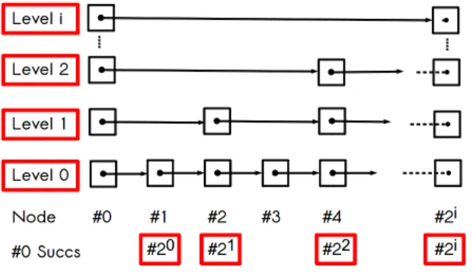
Figure 4.1: Skip links for element #0 within a perfect skip list
Skip list. A skip list is basically an ordered doubly linked list, where in addition to links to direct
successor and predecessor, each skip list element (called node) have also other links to distant successors and predecessors, called distant links or skip links.
In the original version[35]; supposing that the number of nodes is known; skip links are calculated in such a way to ensure that searching any value in the skip list will take a logarithmic time relative to the num-ber of skip list nodes. Indeed, each node will calculate a link to its 2ith successor until reaching the last
element. In the general case where the number of nodes is not known or changes over time, the author, in the same paper proposes a probabilistic version to ensure the same complexity with a high probability. To implement the skip list, we used a deterministic algorithm, inspired from [32], to calculate skip links to have a perfect skip list. Figure 4.1 shows links that a node (node ♯0) must calculate to have a perfect skip list. Note that in the figure only successors links are shown for reason of clarity. Also we will use the term neighbor to designate at the same time a successor and a predecessor. So in the deterministic version, skip links are organized in levels. The first level contains link to to the first (or direct) neighbor. At each level i the skip links are pointing to a neighbor that is two times distant than the neighbor at level i − 1. Therefor each level i calculates a link to the 2ith neighbor until reaching the
last node.
The skip list is well appropriate to implement our distributed structure as it have the required characteristics:
• skip list performances are mainly related to the establishment of the skip links. Rather than the probabilistic version, we use a deterministic version that converges always to the optimal configuration (a prefect skip list),
• as the skip list is a linear structure, its stabilization is more efficient. To ensure that we will use a set of algorithms similar to those used in Chord[39],
• an other interesting point about skip lists, is that the distant links can be also used for fault-tolerance, to recover from faults inducing many successive neighbors.
4.3
Experimental Evaluation
4.3.1 Experiments setupTo join the DHT each new peer first gets an entry peer from the directory that maintains a list of peers participating in the DHT. The DHT data counts more than 12 000 elements and the size of each one is between 5 and 50 Mega bytes. All tests were done using the SimGrid[14] simulator. We first implement a complete CAN DHT , and we implement on top of it the skip list algorithms. SimGrid have many API, we used the GRAS (for Grid Reality and Simulation) API, where the implemented application can be executed in simulation or on real machines.
4.3.2 Results & Discussion
Figure 4.2: Skip list experiments for load-balancing
Figure 4.3: DHT data distribution
Figure 4.2 shows the data load of peers just after building the DHT while using the skip list to insert new peers considering load-balancing criterion comparing to the canonical join algorithm. The data distribution of the DHT is not uniform and is shown in figure 4.3. Each graph traces the cumulative data load of DHT peers, where peers are ordered in the X axis following the decreasing order of their load.
When using the canonical algorithm, graph4.2.a shows that the total DHT data load is managed only by less than the half of peers, where the rest of peers have not practically any data load. However when using the skip list (to consider load-balancing criterion) graph4.2.b shows that all peers participate and have approximatively the same load of data to manage.
5
Data Transfers Minimization
In this chapter we will see how to fast build DHTs by minimizing data transfers while inserting new peers. In the previous chapter we have seen how to insert a new peer considering multiple intra-DHT criteria in the general case. Nevertheless considering extra-DHT criteria, as new peer data transfers minimization, is more difficult. First due to the lack of global view of the DHT, and second the more challenging, that extra-DHT criteria depends on each new peer and can’t calculated until the new peer arrives. So we will see how a new peer can build a partial view more interesting than the local available one. We then use it to develop a heuristic that lets the new peer minimize its input data transfers after being inserted. Yet the heuristic can’t be used for general case. Rather it can be adapted to any extra-DHT criterion that its evaluation depends on available zones and has a bounded objective function. Finally, we present our experimental evaluation and we discuss the results.
5.1
Understanding Data transfers
After a new peer is inserted, there will be some uncontrollable data transfers as the configuration of the DHT has been changed: the responsibility zone of the join peer is narrowed, and the new peer became responsible of a zone of the virtual space. Therefor, first the new peer will receive data form the join peer that it’s no more responsible on it. Second when new peer come with its data, it will send it to the responsible peers for storage.
Those transfers are qualified as uncontrollable as neither the new peer decides where it will store its input data, nor the join peer decides on which data it will pass to the new peer and which ones it keeps. Rather all depends on which sub-zone the join peer will keep and which one it will cede to the new peer, and on where each data element is mapped in the virtual space. Figure5.1 shows this two types of transfers where we call, from the point of view of the new peer:
• incoming data transfers: transfers from the join peer to the new peer, i.e. data that the join peer is no more responsible on,
• outgoing data transfers: transfers from the new peer to the join peer and to other peers, i.e. new peer input data that doesn’t map into its new acquired responsibility zone.
If we define the problematic of data transfers minimization when inserting new peer following our model (see section 3.4), we will have to resolve the following ILP problem:
Figure 5.1: Data transfers when inserting a new peer M in T =P p∈Pγp.(α.Tp + β.Tp′) Tp = T ip+ T op T′ p = T′ip+ T′op γp ∈ {0, 1} and Pp∈Pγp = 1; α, β ∈ {0, 1} and α + β = 1;
where : Tp(resp. Tp′) are data transf ers if new peer choose the
f irst (rep. second) sub zone of peer p
T ip (T op) : incomming (outgoing) data transf ers
P is the set of current DHT peers
(1.3)
So the new peer have to choose the sub-zone that will lead to less data transfers after its insertion. Note that for this criterion; differently than the criterion of load-balancing; we are talking about choosing the sub-zone not the join peer, as the criterion of data transfers minimization depends on the sub-zone that the new peer will get not the peer itself. Indeed, the sub-zone will automatically decide on the join peer.
In practice. It’s clear that the criterion of data transfers minimization is an extra-DHT criterion
as it depends also on the new peer (data). However, to propose a practical solution, we need to divide it in two sub-criterion:
• Outgoing data transfers minimization: concerns the new peer data t hat it will send to the join peer and other DHT peers. Or inversely, the new peer data that it will not keep after its insertion.
• Incomming data transfers minimization: concerns the data that the new peer will receive from the join peer, as it become under its responsibility.
One of the benefit of this separation is that the sub-criterion of incoming data transfers is intra-DHT as it doesn’t depend on the new peer, but only on the data quantity each proposed sub-zone contains. This is interesting because we know how to deal with such criteria. In the next sections we will see how to consider practically each sub-criterion (or simply criterion).
5.2
Incoming Data Transfers Minimization
To consider incoming data transfers minimization criterion; being intra-DHT; we can well use our dis-tributed structure to get the optimal solution to insert new peers. Even we can consider it with other criteria at the same time. For this case, each peer will have two proposals, where each sub-zone will be associated to the quantity of data it contains. The new peer have then to choose the proposal with minimum value. However, this criterion isn’t very interesting alone, because if we consider it alone, it will minimize data transfers but leads to inefficient DHT. Indeed, new peers will choose sub-zones with empty data and there will be no share of load between peers.
We can think about considering this criterion with the criterion of load-balancing to ensure efficiency, but it still not interesting and non significant as the two criteria are completely contradictory. And considering load-balancing alone will be sufficient enough. In next section we will see how to consider outgoing data transfers minimization which is more interesting and more challenging also.
5.3
Outgoing Data Transfers Minimization
Minimizing new peer data transfers will lead to build operational DHTs very rapidly. We mean by operational DHT, a DHT where all data elements are accessible. Indeed when new peers join the DHT with considerable input data it will take a lot of time to store all the data as each data element need to be forwarded to the responsible peer. So as much the new peer can keep of its input data as the construction of the DHT will be faster.
To do so, the new peer need to get information about available sub-zones to get the one where it will keep the most of its data after it is inserted. As this criterion is extra-DHT, we need to provide those information in short time, as they will be calculated for each new peer. In this section we will see how to build a partial view of the DHT based on zone identification algorithm that provide information about some available sub-zones. After we will see how can we decide on the best sub-zone without the need of the knowledge about all available sub-zones, in some special cases. Using those intermediate results, we will present the heuristic we proposed to minimize new peer outgoing data transfers.
5.3.1 Building partial view
To properly describe the information about existing zones when new peer want to join the DHT, we need first to identify each zone (or sub-zone) uniquely so that the new peer can correctly choose the optimal one.
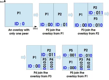
Most of DHTs overlays use the same partitioning procedure: the first peer will get the whole space, and when a new peer joins the DHT, the join peer (the peer that will insert the new one) will split its zone into two parts, and one will be given to the new peer. In fact we can define a deterministic algorithm to identify uniquely any available sub-zone at any time.
Note : In the following, all discussions will be given on CAN DHT as an example, but the ideas and solutions concern DHTs in the general case.
Zones can be identified using binary strings. The whole space will be identified by 0 or 1 following some convention, for example 0 if we start the partitioning over the first dimension (where there is multiple dimension like in CAN). After that we can identify all possible sub-zones using an inductive algorithm : for a zone identified by the bits string b0b1...bn, after it is partitioned, its two sub-zones are
identified by the bits strings b0b1...bn0 and b0b1...bn1. We can adapt a convention so that the choice of
the identifiers for the two sub-zones will be deterministic. For example the sub-zone with lower values (for the partitioning dimension) will have the suffix 0. Figure5.2 show an example of a 2D CAN DHT with 5 peers, and the identification of responsibility zones of each peer over time.
Figure 5.2: Zone identification algorithm. First we give an identifier for the whole space. After each time as a zone is divided new bits are added to create identifiers for the new sub-zones
This identification schema can be seen as a binary tree where each peer represents a zone. Each zone if partitioned will have its two sub-zones as children in the binary tree. Leafs are therefore the actual existing zones and other nodes are zones that no longer exist as they were partitioned before. Figure 5.3 shows an example of a 2D CAN overlay with 5 peers and the corresponding binary tree for zone identification.
Figure 5.3: Zone identification schema tree. Leafs are actual zones managed by overlay peers, and intermediate nodes are old zones that were partitioned.
Using zones identifiers we can get some partial knowledge. Figure 5.4 gives an example on how to get a historical knowledge just by analyzing one zone identifier.
Figure 5.4: How to get a partial view from one zone identifier (0101). The first left bit (0) indicates the first dimension of partitioning, and by analyzing the identifier from left to right, each bit will indicate which sub-zone was partitioned until having the actual zone.
Those informations are historical but still important (especially where there is no leaves and failures) because they give an upper bound of data that the new peer can keep. The heuristic we propose is based on the use of this partial view to get information about the DHT status.
5.3.2 Take Decision based on partial information
We have seen that (in section3.4), to insert a new peer in the optimal position considering an extra-DHT criterion, we need to calculate the objective function for each available sub-zone, and then select the one with the minimal value. This needs to have a global knowledge about DHT -to get all available sub-zones- that we haven’t. However, using the zone identification algorithm we came to get a partial knowledge. So the question now is if we can made a decision on the optimal sub-zone based only on that partial knowledge: how can we take profit from it?
Noticing that, in our problem, that is considering new peer outgoing data transfers, the objective func-tion has an upper bound (all new peer data will be transfered), and the new peer have to select exactly one sub-zone, we can decide that a sub-zone is optimal without calculating the objective function of any other sub-zone in one special case as the following lemma indicates :
Lemma: If for a given sub-zone the new peer will keep more than the half of its data, this zone is the optimal one considering the criterion of outgoing data transfers minimization.
Proof: lets recall how the virtual space I is managed by peers that we saw in the reference definition of DHTs (in section 2.1). At any point in time, I is managed by the set of current peers P. The responsibility for peers for specific identifiers is captured by a function M : I −→ 2P
, which associates with each identifier of a resource r, i = FR(r) ∈ I , the set of peers that are managing r. As we consider
that M is injective and complete, we can see it as a partition of the identifier space I , where each peer p is responsible on a part of I that we call its responsibility zone Zp = M−1(p).
Lets consider SZ the set of all current available sub-zones. SZ forms also a partition of I as each two sub-zones proposed by the same peer are a partition of its responsibility zone. Lets define the function T : SZ −→ R that associates to each sub-zone z the quantity of data, T (z), the new peer will keep if it selects z as its responsibility zone. Its clear that the function T is bounded by TM AX the quantity of
transfers where the new peer will loose all its data. So if the new peer will choose a sub-zone z′ where it will keeps more than the half of its data, i.e. T (z′) ≥ (T
M AX/2), z′ is the optimal sub-zone it can
get when looking to minimize its data transfers. Because, as the new peer can choose only one sub-zone from SZ, and SZ is a partition of the virtual space I any other sub-zone will keeps at most the half of its data.
follow: M ax T =P z∈SZ(γz.T (z)) γz ∈ {0, 1} and Pz∈SZγz = 1 (1.4)
If we have for a given sub-zone z′, T (z′) > (T
M AX/2) and knowing that the objective function T 6 TM AX,
we will have for the rest of sub-zones P
z∈SZ/{z′}(γz.T (z)) 6 (TM AX/2) as T = Pz∈SZ/{z′}(γz.T (z)) +
γz′.T (z′). So choosing z′, i.e. γz′ = 1 and for z ∈ SZ/{z′}, γz = 0, is the best solution to the ILP.
Figure 5.5 illustrates that on an example.
Figure 5.5: When minimizing new peer outgoing data transfers, the zone where the new peer will keep the half or more of its data, is the optimal one.
5.3.3 Heuristic for outgoing data transfers minimization (ODMH)
Now, having a partial view of the DHT built using zone identifiers, and the possibility to take a decision based on partial knowledge, we can propose a heuristic for the new peer so that it can choose the zone that minimize its outgoing data transfers.
In short, the idea of the heuristic is to get a partial view (about existing sub-zones) in the parts of the space where the new peer have most of its data. If the new peer data is very skewed; and then almost all data will be located in one place; the optimal solution will be very probably one of the sub-zones of the built partial view. Else if the new peer have its data located in different areas in the virtual space, the heuristic try to choose the best place to select and fetch for a good sub-zone. Finally if the new peer data is uniform over the virtual space, there will be no considerable gain between sub-zones, and we want to avoid useless calculation by choosing one sub-zone randomly to insert the new peer.
The heuristic proceed following next steps :
1. Be in the right position. Its clear that the partial partial knowledge we can get depends on
the zones that we analyzed. So for the new peer, to keep most of its data it needs to get information about how the virtual space is organized in the area where most of its data is located.
To do so, the new peer will first do a lookup for the [point that represents the] centroid of its data and it will get as a response the zone identifiers of the responsible peer and of its neighbors. If we call new peer data set DataN ewP eer where each data element is represented by the point where it is mapped

![Figure 2.1: Reference definition of Structured Overlay network[10].](https://thumb-eu.123doks.com/thumbv2/123doknet/14425189.706790/12.918.261.656.676.887/figure-reference-definition-of-structured-overlay-network.webp)