Copyright © 2013 Inderscience Enterprises Ltd.
Application of tolerance approach to fuzzy goal
programming to aggregate production planning
Mohammed Mékidiche,
Hocine Mouslim
and Abdelkader Sahed
University of Tlemcen,Annexe Universitaire de Maghnia, BP-600, Maghnia, Wilaya de Tlemcen, Algeria
Fax: 0021340922539 E-mail: [email protected] E-mail: [email protected] E-mail: [email protected] *Corresponding author
Abstract: This study presents the application of a tolerance approach to the fuzzy goal programming (FGP) developed by Kim and Whang (1998) and revised by Yaghoobi and Tamiz (2007-a) to aggregate production planning (RKW-APP) in a state-run enterprise of iron manufactures non-metallic and useful substances (Société des bentonites d’Algérie-BENTAL). The proposed formulation attempts to minimise total production and work force costs, inventory carrying costs and costs of changes in labour levels. A real-world industrial case study in demonstrating the applicability of the suggested model to practical APP decision problems is also given. The LINGO computer package has been used to solve the fi nal crisp linear programming problem package and get an optimal production plan.
Keywords: aggregate production planning; fuzzy goal programming; tolerance approach.
Reference to this paper should be made as follows: Mekidiche, M., Mouslim, H., Sahed A. (2013) ‘Application of tolerance approach to fuzzy goal programming to aggregate production planning’, Int. J. Mathematics in Operational Research, Vol. 5, No. 2, pp.183–204.
Biographical notes: Mékidiche Mohammed is currently an Assistant Professor in the Faculty of Economics and Commerce, University of Tlemcen, Maghnia Annex, Algeria, where he teaches statistics and econometrics, operations research, applied microeconomics and production planning, He received his MS and PHD in production and operations management from the Economics and Commerce Faculty , University of Tlemcen in Algeria. His research project is optimisation in production planning, multi criteria decision making and fuzzy sets theory, fuzzy goal programming, quality control, time series analysis and its application in forecasting, neural network and its application in management. He has published several articles in journals.
Mouslim Hocine is currently an Assistant Professor in the Faculty of Economics and Commerce, University of Tlemcen, Maghnia Annex, Algeria, where he teaches operations research, goal programming, decision making theory and fuzzy set theory. He holds an MSc and PHD in production and operations management from the Economics and Commerce Faculty, University of Tlemcen in Algeria. His research interests are in operations research, goal programming, multi criteria decision making, quality control and fuzzy sets theory. He has published several articles in journals.
Sahed Abdelkader is an Assistant Professor of Economics at the Faculty of Economics and Commerce, University of Tlemcen, Maghnia Annex-Algeria. He holds a Master’s Degree in production and operations management from Tlemcen University (2006), and is currently a PhD candidate in the fi eld of production and operations management at the University of Tlemcen. He teaches courses in statistics, probability, and cconometrics. His research interests include decision making, goal programming, fuzzy sets, operation and production management and econometrics.
1 Introduction
Aggregate production planning (APP), sometimes called intermediate-range planning, involves production planning activities for six months to two years with monthly or quarterly updates. Changes in the workforce, additional machines, subcontracting, and overtime are typical decisions in APP.
The problem with APP concerns management’s response to fl uctuations in the demand pattern. Specifi cally, how can productivity, manpower and goods resources best be utilised in the face of changing demands to minimise the total cost of operations over a given planning horizon?
In response to changing demands, management can utilise the following strategies: • adjust the work force through hiring and fi ring
• adjust the production rate through overtime and under-time absorb the demand fl uctuation rate through inventory back logging or by allowing lost sales
• the production rate may be kept on a constant level and the fl uctuations in demand met by altering the level of subcontracting.
Clearly, each of the above pure strategies implies a set of costs that may be both direct and opportunity. Changing the work force implies costs associated with hiring and layoff. Production rate changes entail costs of overtime and idle resource. Excess inventories require capital investment as well as direct costs, while shortages imply lost revenue and customer goodwill.
Any combination of these preceding strategies is, of course, also possible. The problem with APP is to select the strategy with least cost to the fi rm. This problem has been under extensive discussion, and several alternative methods for fi nding an optimal solution have been suggested in the literature.
2 Literature review
There are numerous methods available in the literature for APP. since Holt et al. (1955) proposed the HMMS rule in 1955, researchers have developed numerous models to help to solve the APP problem, each with its own pros and cons. According to Saad (1982), all traditional models of APP problems may be classifi ed into six categories: (1) linear programming (LP) (Charnes and Cooper, 1961; Singhal and Adlakha, 1989); (2) linear decision rule (LDR) (Holt et al., 1955); (3) transportation method (Bowman, 1956); (4) management coeffi cient approach (Bowman, 1963), (5) search decision rule (SDR) (Taubert, 1968); and (6) simulation (Jones, 1967). When using any of the APP models, the goals and model inputs (resources and demand) are generally assumed to be deterministic/crisp, and only APP problems with the single objective of minimising cost over the planning period can be solved. The best APP balances the cost of building and taking inventory with the cost of the adjusting activity levels to meet fl uctuating demand.
Masud and Hawang (1980) were the fi rst to propose an APP model for the multiple product, single facility case where confl icting multiple objectives are treated explicitly. Three multiple decision-making methods are used to solve this problem, among them the Goal Programming (GP) model developed by Charnes and Cooper (1961).
In practice, the input data in the APP problem , as also data on demand, resources and cost as well as the objective function are frequently imprecise/fuzzy because some information is incomplete or unobtainable. Traditional mathematical programming techniques clearly cannot solve all fuzzy programming problems. Zimmerman (1976) fi rst introduced the fuzzy set theory into conventional LP problems.
Many aspects of the APP problem and the solution procedures employed to solve APP problems lend themselves to the fuzzy set theory approach. Fuzzy APP allows the vagueness that exists in determining forecasted demand and the parameters associated with carrying charges, backorder costs, and lost sales to be included in the problem formulation. Fuzzy linguistic ‘f-then’ statements may be incorporated into the APP decision rules as a means for introducing the judgment and past experience of the decision maker into the problem. In this fashion, the fuzzy set theory increases the model’s realism and enhances the implementation of APP models in the industry. The usefulness of the fuzzy set theory also extends to multiple objective APP models where additional imprecision due to confl icting goals may enter into the problem.
Wang and Fang (2001) present a novel fuzzy linear programming method for solving the APP problem with multiple objectives where the product price, unit cost to subcontract, work force level, production capacity and market demands are fuzzy in nature. An interactive solution procedure is developed to provide a compromise solution.
Reay-ChenWang and Tien-Fu Liang (2005) have developed a fuzzy multi-objective linear programming model for solving the multi-product APP decision problem in a fuzzy environment. Their formulation attempts to minimise total production costs, carrying and backordering costs and costs of changes in labour levels considering inventory level, labour levels, capacity, warehouse space and the time value of money.
Abouzar Jamalnia and Mohammad Ali Soukhakian (2009) have developed a hybrid (including qualitative and quantitative objectives) fuzzy multi-objective non-linear programming model with different goal priorities for solving an APP problem in a fuzzy environment. The proposed model tries to minimise total production costs, carrying and back ordering costs and costs of changes in the workforce level (quantitative objectives) and maximise total customer satisfaction (qualitative objective) with regard to the inventory level, demand, labour level, machine capacity and warehouse space their formulation based on FGP developed bay Chen and Tsai (2001).
This study presents an application of the APP-based A tolerance approach to the fuzzy goal programming (FGP) developed by Kim and Whang (1998) and Revised by Yaghoobi and Tamiz (2007-a) and its application in the national fi rm of iron manufactures non- metallic and useful substances for solving the problems of the APp. The proposed model minimises total production and work force costs, cost of inventory and minimises the degree of change in the work force.
3 Basic structure of the GP model 3.1 Defi nition and literature of GP
The initial development of the concept of GP was due to Charnes and Cooper, in a discussion which took place in 1961, although they claim that the idea actually originated in 1952. In essence, they proposed a model and approach for dealing with certain linear programming
problems in which confl icting “goals of management were included as constraints (Ignizio, 1976; Romero, 1991).
The essential activity of a manager is decision-making. This activity is becoming more complex because managers (decision-makers) try to integrate into their own decisions many different factors. Multiple-criteria problems in conferences, in academic publications and in practice have increased in importance (Martel and Aouni, 1990). GP can be considered to be a mathematical programming method and a member of the multi-criteria decision-making MCDM family. GP constitutes of a modifi cation and extension of linear programming. These two programming techniques are similar to the fact that they both represent optimal solutions to goals and constraints. Nevertheless, GP and linear programming have signifi cant performance differences that give the advantage to GP, which is due to the greater scale of problems that is applied (Zeleny, 1981, 1982).
GP is a multi-objective programming (MOP) technique. GP is based on the distance function concept (Romero, 1991). It later became the most popular model of the MOP. Its popularity is due to the fact that it is a simple model, easy to apply, and takes advantage of the extensive number of mathematical programming software available in the market (Aouni and Kettani, 2001).
Until the middle of the 1970s, GP applications reported in the literature were rather scarce. Since that time, and chiefl y due to seminal works by Lee (1972) and Ignizio (1976), an impressive boom in GP applications and technical improvements has arisen. It can be said that GP has been, and still is, the most widely used multi-criteria decision-making technique (Romero, 1991). Although Schniederjans (1995) has detected a decline in the life cycle of GP with regard to theoretical developments, the number of cases along with the range of fi elds to which GP has been, and is still is, applied is impressive, as shown by recent surveys by Romero (1986), Schniederjans (1995) and Tamiz et al. (1993). It has been applied successfully in practice for many years (Jones and Tamiz, 2002). GP models aim to minimise deviations of the objective values from aspiration levels specifi ed by decision maker(s) (Yaghoobi and Tamiz, 2007-b). The variants of GP are numerous, and contain many different sub-areas which can bewilder practitioners with no knowledge of GP, but wish to apply it to their multi-objective real world situation (Tamiz et al., 1998).
3.2 Formulation of the GP model
Before we can defi ne the GP model, it is absolutely essential to establish precise defi nitions for certain keywords and concepts. This is particularly critical where such defi nitions differ or must be made sharper than in conventional mathematical programming. Now, since the defi nitions of such terms as variables (i.e., controllable/noncontrollable; continuous/discrete), functions (i.e., linear and nonlinear); equations inequalities; and mathematical models are the same as in the multi-objective area, we may move directly to the following set of defi nitions (Ignizio, 1983).
– Objectives: objectives are represented by mathematical functions of their decision or control variables. Such functions usually represent some desire or wish of the decision maker(s). It is important to note that the value of an objective function is left unspecifi ed. The two most common objective function forms are: maximise f(x) or minimise f(x). – Aspiration level: an aspiration level is a specifi c (realistic) value (or ‘target’ level) associated with a desired or acceptable level of achievement of an objective. Thus, an aspiration level may be used to measure the achievement or non-achievement of an objective.
– Goal: an objective in conjunction with an aspiration level is termed a goal. That is, if we say that we wish to maximise profi t, then that is an objective.
However, if we instead, wish to achieve a profi t level of at least $1000, we have established a goal. The mathematical form of a goal is either:
( ) , ( ) , ( ) satisfy f x b or satisfy f x b or satisfy f x b ≤ ≥ =
depending on the situation.
– Constraint: a constraint has exactly the same mathematical appearance as a goal. However, in multi-objective mathematical programming, a constraint is a subset of the concept of goals. In specifi c, a constraint is an infl exible (or rigid or hard) goal. Thus, when a truly infl exible constraint is encountered, we shall denote this relationship as a rigid constraint or, alternately, as an infl exible or absolute goal.
In conventional (i.e., single objective) mathematical programming, we did not have to worry about the distinctions between objectives and goals, or between goals and rigid constraints, as there we dealt with only objectives and (rigid) constraints. However, in multi-objective mathematical programming, precise, non-ambiguous defi nitions are necessary and, in fact, help to form the basis of the power and fl exibility of many of the multi-objective methods.
As we have noted in the previous section, generalised GP encompasses any method which converts the baseline model of into a model consisting solely of goals (some fl exible and some rigid). This is the single, distinguishing feature of generalised GP. The distinction between various types of generalised GP is made on the basis of how one actually measures the ‘goodness’ of any solution (value of b) to the set of goals. This is typically facilitated by means of the concepts of ‘goal deviations’ and the ‘achievement function’.
– Goal deviations: There are, as discussed, three forms of goals: f (x) < b, f (x) > b, and f (x) = b. Since we are using the philosophy of ‘satisfi cing’, we are only interested (at least initially) in measuring the non-achievement of each goal. This is the unwanted deviations from the aspiration levels (i.e., the value of each ‘b’). We let d be the deviation from the goal aspiration and, since such deviation may be either a negative or a positive value d, we let: d = n + p, where n* p = 0 and n, p > 0.
Typically, ni is known as the negative deviation of goal i, while pi, is the positive
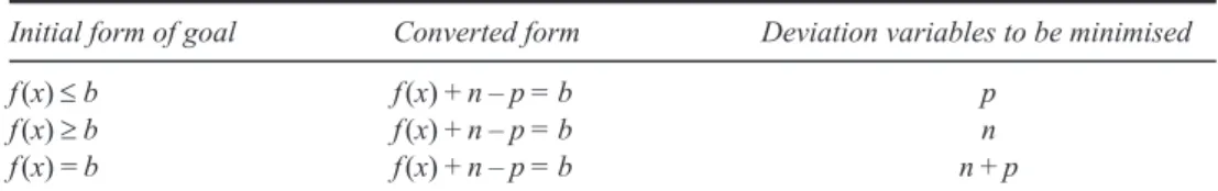
deviation. Thus, to satisfy a specifi c goal, we attempt to minimise the unwanted component (or components) of the goal deviation. This is summarised in Table 1, below:
Table 1 Goals and coal deviations
Initial form of goal Converted form Deviation variables to be minimised
f (x) ≤ b f (x) + n – p = b p
f (x) ≥ b f (x) + n – p = b n
f (x) = b f (x) + n – p = b n + p
Charnes and Cooper (1961) illustrated how that deviation could be minimised by placing the variables representing deviation directly in the objective function of the model. This allows
multiple goals to be expressed in a model that will permit a solution to be found. Multiple and confl icting goals are a distinguishing characteristic to describe how a GP model differs from a linear programming model.
– Model: Charnes and Cooper (1978) presented a generally accepted statement of a GP model, as follows: 1 ( ) : ( ) 1,..., ( int ) , , 0, 1,...., 1,..., k i i i i j i i i x i i j Min Z n p Subject to f x n p b for i k C c system constra s n p x for i k j m = = + + − = = ≤ ≥ = =
∑
(1)ni: is called a positive deviation variable or over-achievement of goal bi.
pi: is called a positive deviation variable or over-achievement of goal bi.
bi: is the arithmetic value of goal i.
Z: is the sum of all deviations. The deviation variables are related to the functionals where:
1 ( ) ( ( )) 2 1 ( ) ( ( )) 2 i i i j i i j i i i j i i j n b f x b f x p b f x b f x = − + − = − − −
Then the sum of the deviations gives:
1 1 ( ) ( ( )) ( ) ( ( )) 2 2 ( ) i i i i j i i j i i j i i j i i j n p b f x b f x b f x b f x d b f x + = − + − + − − − = = −
4 Basic structure of Fuzzy Goal Programming (FGP) 4.1 Defi nition and literature review of FGP
GP models have been classified based on the achievement function that is used to combine unwanted deviations (Romero, 2004): (1) weighted GP (also known as ‘non-pre-emptive GP’) where the weighted sum of deviations from the targets are minimised; (2) pre-emptive priority GP (also known as ‘lexicographic GP’), where a deviation from a higher priority level goal is considered to be infi nitely more important than a deviation from a lower priority goal, and (3) MINMAX GP (also known as ‘Chebyshev GP’), where minimisation of the maximum weighted deviation from the target values is sought. However, determining precise aspiration levels for the objectives in real world problems often is a diffi cult task for decision maker(s) (Yaghoobi and Tamiz, 2007-b). In fact, there are many decision-making situations where the DM does not have complete information on some parameters and, in particular, the goal values in the GP model (Aouni et al., 2010).
The literature review reveals that the FGP is one of the GP variants. According to this review, we notice that the majority of the FGP formulations and applications are based on the model developed by Hannan (1981-a, 1981-b).
Bellman and Zadeh (1970) set the basic principles of decision making in fuzzy environments, which have been used as building blocks of fuzzy linear programming. The use of membership functions in the GP based on the fuzzy set theory was fi rst carried out by Zimmerman (1976, 1978, 1983) and Narasimhan (1980). Further extensions were provided by Hannan (1981-a, 1981-b), Ignizio (1982-a), and Tiwari et al. (1987). Since the early 1980s, fuzzy sets have been used in GP models to represent the satisfaction degree of the decision maker with respect to his/ her preference structure (Narasimhan, 1980); Hannan, 1981-a; Tiwari et al., 1987; Mohamed, R.H 1997;, Chen and Tsai (2001); Yaghoobi and Tamiz (2007-b); and to represent uncertain knowledge about a certain parameter (Mohandas et al., 1990, Chanas and Kuchta (2002).
Various approaches to treating the relative importance of goals in FGP models have been developed. Narasimhan (1980) used a combination of linguistically defi ned weights, such as ‘very important’, ‘moderately important’ and achievement degrees of the goals. The weights and achievement degrees are combined by defi ning a membership function for each linguistic weight, where desirable achievement degrees are specifi ed to represent goal importance. Hannan (1981-b) showed that the above composite approach may lead to some contradictory results, and suggested the use of explicitly defi ned weights to represent the relative importance of goals. Hannan (1981-a) proposed a fuzzy logic-based methodology that employs piecewise linear functions, which represent the decision–maker’s satisfaction with attainment of goal values. A target achievement degree is determined for each goal and the problem is converted to a standard GP formulation, where deviations from these target values are minimised using standard pre-emptive, weighted or MINMAX achievement functions. A different approach is proposed by Tiwari et al. (1987). The authors considered an additive FGP model with relative importance of commensurable goals.
The model included a single-objective function defi ned as the weighted sum of achievement degrees of the goals with respect to their target values. Based on piecewise linear approximation (PLA), Yang et al. (1991) have further formulated the problem with fewer variables, which can yield the same solutions as Narasimhan’s and Hannan’s model. Kim and Whang (1998) have proposed an FGP formulation where the concept of tolerances is introduced to express the fuzzy goals of the DM, instead of using the conventional membership functions. Chen and Tsai (2001) proposed an extension of the additive model to consider goals of different importance and pre-emptive priorities, where the relative importance of goals is modelled by corresponding desirable achievement degrees. Recently, Yaghoobi and Tamiz (2007-b) have proposed a more effi cient formulation, and they have highlighted the fact that the model of Kim and Whang (1998) is different from the Hannan (1981-a, 1981-b) model. It is proved that the proposed model is an extension to the Hannan model that deals with unbalanced triangular linear membership functions. In addition, it is shown that the new model is equivalent to a model proposed by Yang et al. (1991).
Until the middle of the 1990s, FGP applications reported in the literature were rather scarce. We list a categorisation of the major applications of the FGP within management and economics below: Curve and response surface fi tting, Media planning, Manpower planning, Programme selection, Project selection, Hospital administration, Academic resource allocation, Municipal economic planning, Transportation problems, Energy/water resources, Radar system design, Sonar system design, Planning in wood products, Portfolio selection,
Determination of time standards, Development of cost estimating relationships, Urban renewal planning, Merger strategies, Multi-plant/product aggregate production loading, BMD systems design, Multi-objective facility location, Free fl ight rockets, Solar heating and cooling, Natural gas well siting and Maintenance level determination. All of these applications have one thing in common: they could be forced into a traditional single-objective model if one so wished. However, those investigating these problems believed that they truly involved multiple, confl icting objectives, and thus, were most naturally modelled as a FGP problem.
4.2 Formulation of FGP
A useful tool for dealing with imprecision is the fuzzy set theory (Zadeh 1965). An objective with an imprecise aspiration level can be treated as a fuzzy goal. Initially, Narasimhan incorporated the fuzzy set theory in GP in 1980 and presented an FGP model (Narasimhan 1980). Hannan simplifi ed Narasimhan’s method to an equivalent simple linear programming in 1981 (Hannan 1981-b). These pioneering works led to extensive research in the use and application of FGP to real life problems.
To solve FGP problems, various models based on different approaches have been proposed. A survey and classifi cation of FGP models has been presented by Chanas and Kuchta (2002). There are three types of fuzzy goals that are the most common. The following FGP model contains these fuzzy goals.
0 , ( ) 1,..., ( ) 1,..., ( ) 1,..., i i O i i O i O S OPT AX b i i AX b i i j AX i j K X C ≈ ≈ ≤ = ≥ = + ≅ = + ∈ (2)
where OPT means fi nding an optimal decision X such that all fuzzy goals are satisfi ed,
)i AX = 1 .... 1,..., n ij j j a x i k = =
∑
, bi is the aspiration level for i.th goal and the symbol ≅ is afuzzifi er representing the imprecise fashion in which the goals are stated.
The integrated use of GP and the fuzzy sets theory has already been reported in the literature. Zimmerman (1976), Hannan (1981-a; 1981-b), Leberling (1981), Rubin and Narasimhan (1984), Tiwari et al. (1987), Wang and Fu (1997), Kim and Whang (1998), Chen and Tsai (2001), Yaghoobi and Tamiz (2007-b), Yaghoobi et al. (2009), Jiminez et al. (2007), Hatami and Tavana (2011) further integrated several fuzzy linear and multi-objective programming techniques.
The approach chosen in this study for application to the problem of APP is similar to the method developed by Kim and Whang (1998) and revised by Yaghoobi and Tamiz (2007-a).
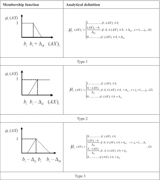
4.3 Membership function
The concept of membership functions, based on the fuzzy set theory, has been introduced and used by Zimmerman (1976; 1978; 1983) and Freeling (1980) for modelling fuzziness related to decision-making context parameters. The general formulation of the membership function used in their formulation is defi ned and depicted as follows (Figure 1, type 1 and type 2).
Narasimhan (1980) and Hannan (1981-a) were the fi rst to give a FGP formulation by using the concept of the membership function. This function is defi ned on the interval [0, 1]. Thus, the membership function for the i – th goal has a value of 1 when this goal is attained, and the decision maker is totally satisfi ed; otherwise, the membership functions assume a value between 0 and 1.
Linear membership functions are used in theory and practice more than other types of membership functions. For the above three types of fuzzy goals, linear membership functions are defi ned and depicted as follows (Figure 1):
Figure 1 Linear membership function and analytical defi nition Membership function Analytical defi nition
µi (AX) 1
b
ib
i+ ∆
iR(AX )
iµ
i 0 1... ..( ) ( ) ( ) .. .. ( ) ... 1,..., ...(1) 0... ..( ) i i i i i i i i iR iR i i iR if AX b AX b AX if b AX b i i if AX b ≤ − = ∆ ≤ ≤ + ∆ = ≥ + ∆ Type 1 µi (AX) 1b
ib
i–
∆
iL(AX )
iµ
i 0 0 1... ..( ) ( ) ( ) .. .. ( ) ... 1,..., ...(2) 0... ..( ) i i i i i i i i iL iL i i iL if AX b b AX AX if b AX b i i j if AX b ≥ − = ∆ ≤ ≤ + ∆ = + ≤ + ∆ Type 2 µi (AX) 1b
i–
∆
iLb
ib
i–
∆
iRµ
i 0 0 0... ..( ) ( ) .. .. ( ) . 1,...., ( ) ...(3) ( ) .. ... ( ) 0... .( ) i i i i i i i iR iR i i i i i i iL iL i i iR if AX b AX b if b AX b i j k AX b AX if b AX b if AX b ≤ − ≤ ≤ + ∆ = + ∆ = − ≤ ≤ + ∆ ∆ ≥ + ∆ Type 3where
∆
iR (or∆
iL) is the quantity of a tolerance in the case of fuzzy goal. This quantity is specifi ed by the decision makers (DMs).4.4 MINMAX approach to FGP problems
In conventional GP problems, the aspiration (target) levels are determined precisely. GP models attempt to minimise the deviations from precise aspiration levels to fi nd an optimal solution for GP problems. Consider a GP problem that is the same as FGP problems, but without the symbol ≈. There exist two major models in GP which are most widely used:
♦ Weighted GP (WGP) ♦ MINMAX GP
MINMAX GP was introduced by Flavell in 1976. This approach minimises the maximum deviation from any single goal. It provides an optimal solution that represents the most balanced solution among the achievements of different goals. Hannan(1981-a) introduced the fi rst MINMAX approach to FGP based on the MINMAX GP developed by Flavel (1976). He considered all fuzzy goals of type 3, Figure 1, with isosceles triangular membership functions (∆iR = ∆iL = ∆i). The linear programming for this special case of FGP
problems is as follows: : ( ) ( 1, 2,... ) 1 ( 1, 2,... ) , 0 i i i i i i i i i i Max Z subject to f x g for i p for i p x X and µ δ δ µ δ µ δ δ − + − + − + = ∆ + − = ∆ = + + δ ≤ = ∈ ≥ (3)
where µ is the degree of membership function.
Despite the fact that the FGP model allows imprecision modelling related to goals values, this model seems to be rigid. Ignizio (1982-b) stresses the fact that Narasimhan and Hannan’s formulations are limited to specifi c cases where the decision maker (DM) is supposed to have membership functions of particular forms like the triangular one. The use of such triangular membership functions was mainly criticised by Ignizio (1982-b) and Martel and Aouni (1998). These criticisms are related to the fact that the triangular form of membership functions does not adequately refl ect the DM’s preferences, and are not an appropriate way for modelling the goal’s fuzziness. Wang and Fu (1997), Pal and Moitra (2003) and Chen and Tsai (2001) have some concerns regarding the way to deal with goals fuzziness through the triangular form of the membership functions, and indicate that in some applications, this type of function leads to non-desirable results.
4.5 Weighted additive FGP (WAFGP)
Hannan (1981-a, 1981-b) introduced the fi rst weighted FGP. He considered all fuzzy goals of type 3, Figure 1, with isosceles triangular membership functions (∆iR = ∆iL = ∆i). The linear
1 ( ) : ( ) ( 1, 2,... ) 1 ( 1, 2,... ) , 0 P i i i i i i i i i i i i i i Min Z w n w p subject to f x n p b for i p n p for i p x X n and p λ λ − + = = + ∆ + − = ∆ = + + ≤ = ∈ ≥
∑
(4) where wi + and w i– are the relative importance coeffi cients associated with the positive and
the negative deviations, respectively. These weights refl ect, partially, the importance that the decision maker (DM) can express differently, depending on whether there is an over- or an under-achievement of the objective.
Tiwari et al. (1987) proposed an alternative formulation based on an WAFGP. They use the addition as an operator to aggregate the weighted membership function values. In their model, only fuzzy goals of types (1-2) are considered. Their model with the notations used in this paper is as follows:
1 0 0 . ( ) 1 1,..., ( ) 1 1,..., 0 1 1,..., K i i i i i i iR i i i iL i S Max Z w st AX b i i b AX i i K i K X C µ µ µ µ = = − = − = ∆ − = − = + ∆ ≤ ≤ = ∈
∑
(5)In Yaghoobi and Tamiz (2006), it is proved that model (5) sometimes yields suboptimal solutions and model (6) overcomes this weakness. Another advantage of model (6) is that in the optimal solution μi determines the degree of membership function for the i th fuzzy goal.
1 0 0 . ( ) 1 1,..., ( ) 1 1,..., 0 1 1,..., K i i i i i i iR i i i iL i S Max Z w st AX b i i b AX i i K i K X C µ µ µ µ = = − ≤ − = ∆ − ≤ − = + ∆ ≤ ≤ = ∈
∑
(6)Among the most important criticism of previous models is that they do not use all types of membership functions, but only use type 1 and type 2, which makes them of limited use in some applications. They do not incorporate the DM’s preferences.
4.6 A tolerance approach to FGP (RKW model)
Kim and Whang (1998) have proposed another approach based on the weighted additive model for solving FGP problems with unequal weights, which can be formulated as a single LP problem with the concept of tolerances. They attempted to extend the Hannan (1981-b) model by introducing an LP model that is able to handle unbalanced triangular linear membership functions. The Kim and Whang (KW) model for FGP can be formulated as follows: 0 0 0 1 1 1 0 0 0 0 _ ( ) : ( ) 1,..., ( ) 1,..., ( ) 1,..., , 0 1,...., ; j io k i i i i i i i i i i i j i iR i i i iL i i i iL i iR i i i i S Min Z w w w st AX b i i AX b i i j AX b i j K i K X C β β β β β β β β β β + − + − = = + = + + − − + + = + + + − ∆ ≤ = + ∆ ≥ = + + ∆ − ∆ = = + ≥ = ∈
∑
∑
∑
(7)where wi is the weight of the ith goal and βi
+ and β
i
– are the positive and negative deviational
variables.
However, Yaghoobi and Tamiz (2007-a), in a recent note, have shown that this model can yield undesirable results in comparison with the Hannan (1981-b) model. It is suggested to insert the following constraints into the model:
0 0 0 0 1... 1,..., 1... 1,..., 1... 1,..., i i i i i i i i j i j K β β β β + − + − ≤ = ≤ = + + ≤ = + (8)
Model (7) augmented with (8) is called the revised Kim and Whang (RKW) model.
• The operator (min sum of tolerances: max sum of all goals membership degrees) of the RKW model is more suitable to unbalanced development planning than the max–min operator of other FGP models. That is because in solving a FGP problem, the feasible solution region approached by the RKW model is larger than or equal to those of the other FGP models like Narasimhan (1980), Hannan (1981-b), Yang et al. (1991) and Tiwari et al. (1987). If we solved a given FGP problem, the sum of the membership degrees of the optimal solution achieved by the RKW model would be better than or equal to those of the other FGP models.
• In addition, when comparing degree differences between the grade of membership for the best satisfi ed goal and the grade for the worst satisfi ed goal, the difference solved by the RKW model is greater than or equal to those by other FGP models.
• The RKW model can be used for types 1–3 of membership functions. 5 Multi-objective programming (MOP) model to APP
5.1 Parameters and constants defi nition
vit: production cost for product i in period t, excluding labour cost in period t (units)
cit: inventory carrying cost for product i between period t and t + 1
rt: regular time work force cost per employee hour in period t
dit : forecast demand for product i in period t (units)
Kit: quantity to produce one worker in regular time for product i in period t
Iio: initial inventory level for product i (units)
T: horizon of planning
N: total number of products Pit: quantity of i product to the period t
Iit: inventory level for product i in period t (units)
Ht: worker hired in period t (man)
Ft: workers laid off in period t (man)
Iit.Min: minimum inventory level available for product i in period t (units)
Wt: total strength of work force level in period t (man)
WMin: the minimum work force level (man) available in period t
WMax: the maximum work force level (man) available in period t
5.2 Objective functions
Masud and Hwang (1980) specifi ed three objective functions to minimise total production costs, carrying and backordering costs and costs of changes in labour levels. In this study, we propose a model that will be using two strategies, where they are available, in a national fi rm dealing in iron manufactures and non-metallic and useful substances. In their multi-product APP decision model, the three objectives of the APP model can be formulated as follows:
•
Minimise total production costs1 1 1 1 . N T ( it it) T (t t) i t t Min Z v P rW = = = ≅
∑∑
+∑
The production costs include: regular time production, overtime, carrying inventory, and specify the costs of change in work force levels.
•
Minimise costs of changes in labour levels2 1 . T t t t t Min Z h H f F = ≅
∑
+•
Minimise carrying costs3 1 . T ( it it) t Min Z c I = ≅
∑
.where the symbol ≅ is the fuzzifi ed version of = and refers to the fuzzifi cation of the aspiration levels.
The objective functions of the APP model in this study assume that the DM has such imprecise goals as, the objective functions should be essentially equal to some value. These confl icting goals are required to be simultaneously optimised by the DM in the framework of fuzzy aspiration levels.
5.3 Constraints
•
The inventory level constraints: Pit + Ii,t–1 – It = dtIit > Iit.Min
•
Constraints on labour levels: Wt – Wi–1 – Hi + Ft = 0WMin < Wt < WMax
•
Constraints on labour capacity in regular and overtime: Pit – Kt * Wt < 0•
Non-negativity constraints on decision variables: Pit , It, Wt, Ht, Ft > 06 RKW model for APP (RKW-APP)
We will use the method that was developed by Kim and Wahang (1998) (models 7, 8) and revised by Yahgoobi and Tamiz (2007-a) (constraint 6) for formulating the APP problem with fuzzy gaols. The complete RKW-APP model can be formulated as follows.
3 4 1 1 1 1 2 2 2 3 3 3 : ( cos ) ( cos ) ( cos ) i i i IR IR IR Min Z w ST
Z b Minimize total production ts
Z b Mininmize tes of changes in labor leveles
Z b Minimize carying ts β β β β + = + + + = − ∆ ≤ − ∆ ≤ − ∆ ≤
∑
, 1 it i t it it X +I − −I =d . it it Min I ≥I 1 0 t t t t W W− − −H +F = Min t Max W ≤W ≤W* 0 it it t P −K W ≤ βi+ < 1 Pit, Iit, Wt, Ht, βi+ > 0 7 Model implementation
7.1 An industrial case study and data description
In this section, as a real-world industrial case, we use a data set provided by the national fi rm dealing in iron manufactures, non- metallic and useful substances (BENTAL) in Algeria. This company manufactures three types of products which are important, and one of the raw materials used in many industries, with bentonite (BEN), carbonate of calcium (CAL) and discolouring (TD). The fi rm employs 175 workers, and the system of work in the fi rm is continuous production (8 × 3 hours) for all days of the week except Thursday, a half-working day and Friday, which is a rest day. Production management is composed of 68 workers divided into 3 groups.
The demand for the products of the individual fi rm in the production of mineral products mentioned above is large, which may cause problems in the productive capacity of this fi rm. Figure 2 show fl uctuations in demand on the level of monthly production capacity of any production capacity (CAP).
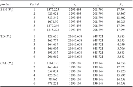
Therefore, the impact on the level and volatility of productive capacity calls for the fi rm, in an attempt to develop a plan of production, to try to cope with fl uctuations in demand due to seasonal changes. Table 2 summarises the basic data gathered from the fi rm. The proposed model implementation in the company has the following conditions:
1 There is a six-month period planning horizon. 2 A three product situation is considered.
3 The initial inventory in period 1 is I10 = 1857tons of BEN, I20 = 1029tons of TD and
I30 = 1860 tons of CAL.
4 Minimum inventory that must be maintained during the period t of product i is 500. Tons.
5 The costs associated with hiring and layoff, according to estimations of the human resource management department, are respectively 51,780 DA/man and 41,550 DA/man. 6 The cost of one worker in the production of three products during the t period is rt =
26940.706.DA/man.
7 The minimum work force level (man) available in each period is WMin = 55workers.
8 The maximum work force level available in each period is WMax = 68workers.
9 The initial worker level is (W0 = 56).
10 The maximum capacity of storage of the 3 products in the fi rm is 6,000 tons. 11 The board of directors of the fi rm has set four business goals as follows:
• Goal 1: The total production cost is about 32,500,000 DA, with positive tolerance of 1,000,000 DA.
• Goal 2: The total cost of changes in labour levels is about 0 DA, with positive tolerance of 100,000 DA.
• Goal 3: The total carrying cost is about 435,000 DA with positive tolerance of 250,000 DA.
Figure 2 The fl uctuation of the actual demand on the level of production capacity for TD, BEN, CAL
Table 2 The basic data provided by the Bental fi rm (in units of Algeria dinar DA (1US$≅ 100DA))
product Period dit vit cit Kit BEN (P1t) 1 1377.225 3293.493 208.796 17.794 2 923.021 3293.493 208.796 15.367 3 883.342 3293.493 208.796 18.602 4 1071.99 3293.493 208.796 16.985 5 1379.269 3293.493 208.796 17.794 6 1315.222 3293.493 208.796 17.794 TD (P2t) 1 128.620 21646.608 848.721 3.883 2 163.777 21646.608 848.721 3.353 3 164.617 21646.608 848.721 4.059 4 166.005 21646.608 848.721 3.706 5 193.317 21646.608 848.721 3.883 6 206.662 21646.608 848.721 3.883 CAL (P3t) 1 1164.191 1296.109 139.149 14.558 2 463.447 1296.109 139.149 12.573 3 659.034 1296.109 139.149 15.220 4 425.240 1296.109 139.149 13.897 5 78.967 1296.109 139.149 14.558 6 478.221 1296.109 139.149 14.558
7.2 Formulation of the RKW-APP
Based on the above information, and using a method (RKW) developed by Kim and Whang (1998) and revised by Yaghoobi and Tamiz (2007-a), the FGP formulation in this study as follows:
4 1 2 3 1 1 1 3 3 3 Min Z = β++ β++ β+ Subject to: 1 1 2 2 3 3 1000000 32000000 100000 0 250000 4350000 Z Z Z β β β + + + − ≤ − ≤ − ≤ , 1 1 0 0 it it t it i t it it t t t t P K W P I I d W W H F − − − × ≤ + − = − − + = 3 1 6000 Min t Max it i W W W I = ≤ ≤ ≤
∑
500 it I ≥ 1 2 3 1 1 1 β β β + + + ≤ ≤ ≤ 10 20 30 0 1856.25 1029 1860 68 I I I W = = = = Pit, Iit, Wt, Ht, Ft, B1+, B2+, B3+ > 0 i = 1, 2, 3 t = 1, 2.,..., 6 Wt , Ht , Ft (integers).7.3 Solving the RKW-APP problem
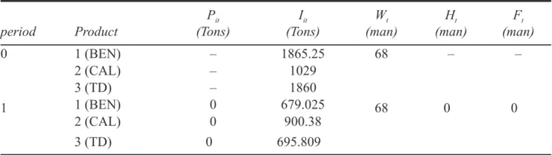
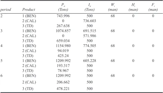
The LINGO computer software package was used to run the Linear programming model. Table 3 presents the optimal aggregate production plan in the industrial case study based on the current information.
Using the RKW-APP to simultaneously minimise total production costs (Z1), costs
of changes in labour levels (Z2) and carrying costs (Z3) yields total production cost of
32,032,504.2 DA, and carrying cost of 4,375,292.99 DA and costs of changes in labour levels of 0. The resulting deviational value for the three fuzzy goal (β1
+, β 2
+ and β 3
+) are
0.0371, 0 and 0.102 respectively; this means that the membership degrees of the three goals are 0.968, 1 and 0.898, respectively.
Table 3 Optimal production plan in the BENTAL fi rm case with the RKW-APP model
period Product Pit (Tons) Iit (Tons) Wt (man) Ht (man) Ft (man) 0 1 (BEN) – 1865.25 68 – – 2 (CAL) – 1029 3 (TD) – 1860 1 1 (BEN) 0 679.025 68 0 0 2 (CAL) 0 900.38 3 (TD) 0 695.809
period Product Pit (Tons) Iit (Tons) Wt (man) Ht (man) Ft (man) 2 1 (BEN) 743.996 500 68 0 0 2 (CAL) 0 736.603 3 (TD) 267.638 500 3 1 (BEN) 1074.857 691.515 68 0 0 2 (CAL) 0 571.986 3 (TD) 659.034 500 4 1 (BEN) 1154.980 774.505 68 0 0 2 (CAL) 94.019 500 3 (TD) 425.24 500 5 1 (BEN) 1209.992 605.228 68 0 0 2 (CAL) 193.317 500 3 (TD) 78.967 500 6 1 (BEN) 1209.992 500 68 0 0 2 (CAL) 206.662 500 3 (TD) 478.221 500
Despite the good results that were obtained through the proposed model, it remains very much sensitive to the accuracy of the information and data provided by the organisation under study.
8 Further scenario designs
This section discusses the actual implementation of the RKW-APP model by considering various alternatives and analysing the sensitivity of decision parameters to variations in relevant conditions, based on the preceding industrial case. The model is implemented in the following seven scenarios.
Scenario 1: Remove Z3 (carrying costs), consider only Z1 (total production costs) and Z2
(costs of changes in labour levels) simultaneously.
Scenario 2: Remove Z2 (costs of changes in labour levels), consider only Z1 (total production
costs) and Z3 (carrying costs) simultaneously.
Scenario 3: Remove Z1 (total production costs), consider only Z2 (costs of changes in labour
levels) and Z3 (carrying costs) simultaneously.
Scenario 4: Analyse the sensitivity by changing the quantity of tolerance for each goal. Table 4 shows the implementation data of scenario 4. In Table 4, positive values indicate increases and negative values indicate decreases in related items in each run.
The results of implementing the previous four scenarios are summarised in Table 5 and Table 6. Signifi cant decision making implications for management that were found after sensitivity analysis of the proposed model are as follows:
Table 4 Implementation data of scenario 4
Scenario Item Run 1 Run 2 Run 3 Run 4
Scenario 4 (Tolerance) ∆iL –30 % –20 % +20 % +30 %
Table 5 Results of implementation in Scenarios 1 to 3
Item Scenario 1 Scenario 2 Scenario 3
β1 + 0.06108 0,09881 – β2 + 0.04155 – 0.10354 β3 + – 0 0.04143 Z1 32561089,6 32598819,5 – Z2 517700 – 103540 Z3 – 435000 4360358,78
Table 6 Results of implementation in scenario 4
Item Run 1 Run 2 Run 3 Run 4
β1 + 0,0453 0.0396 0.0264 0.2440 β2 + 0 0 0 0 β3 + 0,146 0,128 0.085 0.07881 Z1 5475055,55 5475055,55 5475055,55 5475055,55 Z2 4375615,51 4375615,51 4375615,51 4375615,51 Z3 0 0 0 0
• Comparison of scenarios 1–3 demonstrates the interaction of trade-offs and confl icts among dependent objective functions. From Table 5, it is seen that the total production costs, carrying costs, and costs of changes in labour levels have diverse meanings. For instance, the combination of the total production costs and costs of changes in labour levels in scenario 1 was Z1=32,561,089.6 DA and Z2=517,700 DA. Moreover,
the combination of the total production costs and carrying costs in scenario 2 was Z1=32,598,819.5 and Z3=435,000 DA. Finally, the combination of the carrying
costs and costs of changes in labour levels in scenario 3 was Z2=103,540 DA and
Z3=4,360,358.78 DA. These solutions indicate that a fair difference and interaction
exists in the trade-offs and confl icts among dependent objective functions. Different combinations of the arbitrary objective function may infl uence the objective and β1+,
β2– and β3– values. Accordingly, the proposed RKW-APP model meets the requirements
of practical application since it can simultaneously minimise the total production costs, carrying costs, and costs of changes in the labour levels.
• The results of scenario 4 indicate that with increase in the quantity of tolerance for each goal, the value for each objective (Z1, Z2 , Z3) remains constant, and its deviational value
for the three fuzzy goals (β1+, β2+ and β3+) decreases with decrease in the quantity of
9 Conclusions
To conclude our research. we move to present fi rst a brief explanation of APP, which is concerned with determination of production, the inventory and the workforce levels of a company on a fi nite time horizon. The objective is to reduce the total overall cost to fulfi l a situation of inconstant demand, assuming fi xed sales and production capacities.
In this study, we used the tolerance approach to the FGP developed by Kim and Whang (1998) and revised by Yaghoobi and Tamiz (2007-a) for aggregate production planning (RKW-APP). The proposed model attempts to minimise total production and work force costs, carrying inventory costs and costs of changes in labour levels, so that in the end, the proposed model is solved by using the LINGO program and getting the optimal production plan.
Moreover, the major limitations of the proposed model concern the assumptions made in determining each of the decision parameters, with reference to production costs, forecast demand, maximum work force levels, and production resources. Hence, the proposed model must be modifi ed to make it better suited to practical applications. Future researchers may also explore the fuzzy properties of decision variables, coeffi cients and relevant decision parameters in APP decision problems. We will use linear programming with the fuzzy parameters developed by Jiménez et al. (2007) and extended by Marbini.A.H and Tavana M (2011), which will enable us to use the APP problems in cases where the parameters are fuzzy. Acknowledgements
The authors are grateful for the valuable comments and suggestions from the respected reviewers, which have enhanced the strength and signifi cance of our work.
References
Aouni, B., Martel, J.M. and Hassaine, A. (2010) ‘Fuzzy Goal Programming Model: An Overview of the Current State-of-the Art’, Journal Of Multi-Criteria Decision Analysis, Vol. 16, pp.149–161. Aouni, B. and Kettani, O. (2001) ‘Goal programming model: a glorious history and a promising
future’, European Journal of Operational Research, Vol. 133, pp.225–231.
Bellman, R.E. and Zadeh, L.A. (1970) ‘Decision making in a Fuzzy environment’, Management
Science, Vol. 17, No. 2, pp.141–164.
Bowman, E.H. (1956) ‘Production scheduling by the transportation method of linear programming’,
Operations Research, Vol. 4, pp.100–103.
Bowman, E.H. (1963) ‘Consistency and optimality in managerial decision making’, Management
Science, Vol. 9, pp.310–321.
Chanas, S. and Kuchta, D. (2002) ‘Fuzzy goal programming – One notation, many Meanings’, Control
and Cybernetics , Vol. 31, No. 4, pp.871–890.
Charnes, A., Cooper, WW. and Rhodes, E. (1978) ‘ Measuring the effi ciency of decision making units’,
European Journal of Operations Research, Vol. 2, pp.429–444.
Charnes, W. and Cooper, W. (1961) ‘Management Models and Industrial Applications of Linear
Programming’, John Wiley and Sons, New York.
Chen, L-H. and Tsai F-C. (2001) ‘Fuzzy goal programming with different importance and priorities’,
European Journal of Operational Research, Vol. 133, pp.548–556.
Flavell, R.B. (1976) ‘A new goal programming formulation’, Omega, Vol. 4, pp.731–732.
Freeling, A.N.S. (1980) ‘Fuzzy sets and decision analysis’, IEEE Transactions on Systems, Management
Gen, M. and Tsujimura, Y. and Ida, K. (1992) ‘Method for solving multiobjective aggregate production planning problem with fuzzy parameters’, Computers and Industrial Engineering, Vol. 23, pp.117–120.
Hannan, E.L. (1981-a) ‘On Fuzzy Goal Programming’, Decision Sciences, Vol. 12, pp.522–531. Hannan, E.L. (1981-b) ‘Linear programming with multiple fuzzy goals’, Fuzzy Sets and Systems,
Vol. 6, pp.235–248.
Holt, C.C., Modigliani, F. and Simon, H.A. (1955) ‘Linear decision rule for production and employment scheduling’, Management Science, Vol. 2, pp.1–30.
Iginizio, J.P. (1983) ‘Generalized Goal Programming, An Overview’, Computers and Operational
Research, Vol. 10, No. 4, pp.277–289.
Ignizio, J.P. (1976) ‘Goal Programming and Extensions’, Massachusetts, Lexington Books.
Ignizio, J.P. (1982-a) ‘On the (re)discovery of fuzzy goal programming’, Decision Sciences, Vol. 13, pp.331–336.
Ignizio, J.P. (1982–b) ‘Notes and communications of the (re)discovery of fuzzy goal programming’,
Decision Sciences, Vol. 13, pp.331–336.
Jamalnia, A. and Soukhakian, M.A. (2009) ‘A hybrid fuzzy goal programming approach with different goal priorities to aggregate production planning’, Computers and Industrial Engineering, Vol. 56, pp.1474–1486.
Jiménez, M., Arenas, M., Bilbao, A. and Rodríguez, M.V. (2007) ‘Linear programming with fuzzy parameters: an interactive method resolution’, European Journal of Operational Research, Vol. 177, No. 3, pp.1599–1609.
Jones, D.F. and Tamiz, M. (2002) ‘Goal programming in the period 1990–2000’, in Multiple criteria optimization state of the art annotated Bibliographic surveys’, Erghott M. and Gandibleux X. (eds.) Kluwver, pp.129-170.
Jones, C.H. (1967) ‘Parametric production planning’, Management Science, Vol. 13, pp.843–866. Kim, J.S. and Whang, K.S. (1998) ‘A tolerance approach to the fuzzy goal programming problems
with unbalanced triangular membership function’, European Journal of Operational
Research, Vol. 107, pp.614–624.
Lee, S.M. (1972) ‘Goal Programming for Decision Analysis’, Auerbach, Philadelphia, PA.
Marbini, A.H. and Tavana, M. (2011) ‘An extension of the linear programming method with fuzzy parameters’, International Journal of Mathematics in Operational Research, Vol. 3, No. 1, pp.44–55.
Martel, J-M. and Aouni, B. (1990) ‘Incorporating the decision makers preferences in the goal programming model’, Journal of Operational Research Society, Vol. 41, pp.1121–1132.
Martel, J-M. and Aouni, B. (1998) ‘Diverse imprecise goal programming model formulations’, Journal
of Global Optimization, Vol. 12, pp.127–138.
Masud, A.S.M. and Hwang, C.L. (1980) ‘An aggregate production planning model and application of three multiple objective decision methods’, International Journal of Production Research, Vol. 18, pp.741–752.
Mohamed, R.H. (1997) ‘The relationship between goal programming and fuzzy programming’, Fuzzy
Sets and Systems, Vol. 89, pp.215–222.
Mohandas, S.U., Phelps, T.A. and Ragsdell, K.M. (1990) ‘Structural optimization using a fuzzy goal programming approach’, Computers and Structures, Vol. 37, No. 1, pp.1–8.
Narasimhan, R. (1980) ‘Goal Programming in a Fuzzy Environment’, Decision Sciences, Vol. 11, pp.325–336.
Pal, B.B. and Moitra, B.N. (2003) ‘A goal programming procedure for solving problems with multiple fuzzy goals using dynamic programming’, European Journal of Operational Research, Vol. 144, pp.480–491.
Reay-Chen Wang and Tien-Fu Liang (2005) ‘Aggregate production planning with multiple fuzzy goals’, International Journal of Advanced Manufacturing Technology, Vol. 25, pp.589–597.
Romero, C. (2004) ‘A general structure of achievement function for a goal programming model’,
European Journal of Operational Research, Vol. 153, pp.675–686.
Romero, C. (1991) ‘Handbook of Critical Issues in Goal Programming’, Pergamon Press, Oxford. Saad, C. (1982) ‘An overview of production planning model: structure classifi cation and empirical
assessment’, International Journal of Production Research, Vol. 20, pp.105–114.
Schniederjans (1995) ‘Goal Programming: Methodology and Applications’, Kluwer Academic Publishers, Norwell, USA.
Singhal, K. and Adlakha,V. (1989) ‘Cost and shortage trade-offs in aggregate production planning’,
Decision Sciences, Vol. 20, pp.158–165.
Tamiz, M., Jones, D.F. and Romero, C. (1998) ‘Goal programming for decision making: An overview of the current state-of-the-art’, European Journal of Operational Research, Vol. 111, pp.569–581.
Tamiz, M., Jones, D.F. and EL-Darai, E. (1993) ‘A review of Goal Programming and for its application’,
Annals of operations Research, Vol. 58, pp.39–53.
Tang, J., Wang, D. and Fung, R.Y.K. (2000) ‘Fuzzy formulation for multi-product aggregate production planning’, Production Planning and Control, Vol. 11, pp.670–676.
Taubert, W.H. (1986) ‘A search decision rule for the aggregate scheduling problem’, Management
Science, Vol. l4, pp.343–359.
Tiwari, R.N. and Dharmar, J.R. Rao. (1987) ‘Fuzzy goal programming—An additive model’, Fuzzy
Sets and Systems, Vol. 24, pp.27–34.
Wang, H-F. and Fu, C-C. (1997) ‘A generalization of fuzzy goal programming with pre-emptive structure’, Computers Operational Research, Vol. 24, No. 9, pp.819–828.
Wang, R.C. and Fang, H.H. (2001) ‘Aggregate production planning with multiple objectives in a fuzzy environment’, European Journal of Operational Research, Vol. 133, pp.521– 536.
Yaghoobi, M.A. and Tamiz, M. (2007-a) ‘A note on article. A tolerance approach to the fuzzy goal programming problems with unbalanced triangular membership function’, European Journal of
Operational Research, Vol. 176, pp.636–640.
Yaghoobi, M.A. and Tamiz, M. (2007-b) ‘A method for solving fuzzy goal programming problems based on MINMAX approach’, European Journal of Operational Research, Vol. 177, pp.1580–1590.
Yaghoobi, M.A. and Tamiz, M. (2006) ‘On improving a weighted additive model for fuzzy goal programming problems, International Review of fuzzy mathematics, Vol. 1, pp.115–129. Yang, T., Ignizio, J.P. and Kim, H.J. (1991) ‘Fuzzy programming with nonlinear membership functions:
Piecewise linear approximation’, Fuzzy Sets and Systems, Vol. 41, pp.39–53. Zadeh, L.A. (1965) ‘Fuzzy Sets’, Information and Control, Vol. 8, pp.338–353.
Zeleny, M. (1982) ‘Multiple Criteria Decision Making’, McGraw Hill Book Company, New York. Zeleny, M. (1981) ‘The Pros and Cons of goal programming’, Computers and Operations Research ,
Vol. 8, No. 4, pp.357–359.
Zimmerman, H-J. (1983) ‘Using fuzzy sets in operations research’, Fuzzy Sets and Systems, Vol. 13, pp.201–216.
Zimmerman, H-J. (1976) ‘Description and optimization of fuzzy systems’, International Journal of
General Systems, Vol. 2, pp.209–215.
Zimmerman, H.J. (1978) ‘Fuzzy programming and linear programming with several objective functions’, Fuzzy Sets and Systems, Vol. 1, pp.45–56.