Death and rebirth of neural activity in sparse inhibitory networks

HAL Id: hal-01663999

https://hal.archives-ouvertes.fr/hal-01663999

Submitted on 11 May 2018

HAL is a multi-disciplinary open access

archive for the deposit and dissemination of

sci-entific research documents, whether they are

pub-lished or not. The documents may come from

teaching and research institutions in France or

abroad, or from public or private research centers.

L’archive ouverte pluridisciplinaire HAL, est

destinée au dépôt et à la diffusion de documents

scientifiques de niveau recherche, publiés ou non,

émanant des établissements d’enseignement et de

recherche français ou étrangers, des laboratoires

publics ou privés.

networks

David Angulo-Garcia, Stefano Luccioli, Simona Olmi, Alessandro Torcini

To cite this version:

David Angulo-Garcia, Stefano Luccioli, Simona Olmi, Alessandro Torcini. Death and rebirth of neural

activity in sparse inhibitory networks. New Journal of Physics, Institute of Physics: Open Access

Journals, 2017, 19 (5), pp.053011. �10.1088/1367-2630/aa69ff�. �hal-01663999�

PAPER • OPEN ACCESS

Death and rebirth of neural activity in sparse

inhibitory networks

To cite this article: David Angulo-Garcia et al 2017 New J. Phys. 19 053011

View the article online for updates and enhancements.

Related content

Spatiotemporal dynamics of continuum neural fields

Paul C Bressloff

-Neural networks as spatio-temporal pattern-forming systems

Bard Ermentrout

-Exploiting pallidal plasticity for stimulation in Parkinson’s disease

Marcel A J Lourens, Bettina C Schwab, Jasmine A Nirody et al.

-Recent citations

Exact firing time statistics of neurons driven by discrete inhibitory noise

Simona Olmi et al

PAPER

Death and rebirth of neural activity in sparse inhibitory networks

David Angulo-Garcia1,2_{, Stefano Luccioli}3,4_{, Simona Olmi}1,3,5_{and Alessandro Torcini}1,2,3,6,7,8 1 _{Aix Marseille Univ, INSERM, INMED and INS, Inst Neurosci Syst, Marseille, France}

2 _{Aix Marseille Univ, Université de Toulon, CNRS, CPT, UMR 7332, F-13288 Marseille, France}

3 _{CNR—Consiglio Nazionale delle Ricerche—Istituto dei Sistemi Complessi, I-50019 Sesto Fiorentino, Italy} 4 _{INFN—Istituto Nazionale di Fisica Nucleare—Sezione di Firenze, I-50019 Sesto Fiorentino, Italy} 5 _{Weierstrass Institute, Mohrenstraße 39, D-10117 Berlin, Germany}

6 _{Laboratoire de Physique Théorique et Modélisation, Université de Cergy-Pontoise, CNRS, UMR 8089, F-95302 Cergy-Pontoise Cedex,}

France

7 _{Max-Planck-Institut für Physik komplexer Systeme, Nöthnitzer Straße 38, D-01187 Dresden, Germany} 8 _{Author to whom any correspondence should be addressed.}

E-mail:david.angulo-garcia@univ-amu.fr,stefano.luccioli@fi.isc.cnr.it,simona.olmi@isc.cnr.itandalessandro.torcini@univ-amu.fr Keywords: neural network, inhibition, pulse-coupled neural models, lyapunov analysis, leaky integrate-and-fire model, firing statistics

Abstract

Inhibition is a key aspect of neural dynamics playing a fundamental role for the emergence of neural

rhythms and the implementation of various information coding strategies. Inhibitory populations are

present in several brain structures, and the comprehension of their dynamics is strategical for the

understanding of neural processing. In this paper, we clarify the mechanisms underlying a general

phenomenon present in pulse-coupled heterogeneous inhibitory networks: inhibition can induce not

only suppression of neural activity, as expected, but can also promote neural re-activation. In

particular, for globally coupled systems, the number of

firing neurons monotonically reduces upon

increasing the strength of inhibition

(neuronal death). However, the random pruning of connections

is able to reverse the action of inhibition, i.e. in a random sparse network a sufficiently strong synaptic

strength can surprisingly promote, rather than depress, the activity of neurons

(neuronal rebirth).

Thus, the number of

firing neurons reaches a minimum value at some intermediate synaptic strength.

We show that this minimum signals a transition from a regime dominated by neurons with a higher

firing activity to a phase where all neurons are effectively sub-threshold and their irregular firing is

driven by current

fluctuations. We explain the origin of the transition by deriving a mean field

formulation of the problem able to provide the fraction of active neurons as well as the

first two

moments of their

firing statistics. The introduction of a synaptic time scale does not modify the main

aspects of the reported phenomenon. However, for sufficiently slow synapses the transition becomes

dramatic, and the system passes from a perfectly regular evolution to irregular bursting dynamics. In

this latter regime the model provides predictions consistent with experimental

findings for a specific

class of neurons, namely the medium spiny neurons in the striatum.

1. Introduction

The presence of inhibition in excitable systems induces a rich dynamical repertoire, which is extremely relevant for biological[13], physical [32], and chemical systems [84]. In particular, inhibitory coupling has been invoked

to explain cell navigation[87], morphogenesis in animal coat pattern formation [46], and the rhythmic activity

of central pattern generators in many biological systems[27,45]. In brain circuits, the role of inhibition is

fundamental to balance massive recurrent excitation[73] in order to generate physiologically relevant cortical

rhythms[12,72].

Inhibitory networks are important not only for the emergence of rhythms in the brain, but also for the fundamental role they play in information encoding in the olfactory system[39] as well as in controlling and

regulating motor and learning activity in the basal ganglia[5,15,47]. Furthermore, stimulus-dependent OPEN ACCESS

RECEIVED

23 October 2016

REVISED

19 March 2017

ACCEPTED FOR PUBLICATION

29 March 2017

PUBLISHED

16 May 2017

Original content from this work may be used under the terms of theCreative Commons Attribution 3.0 licence.

Any further distribution of this work must maintain attribution to the author(s) and the title of the work, journal citation and DOI.

sequential activation of a group of neurons, reported for asymmetrically connected inhibitory cells[33,52], has

been suggested as a possible mechanism to explain sequential memory storage and feature binding[67].

These explain the long-term interest for numerical and theoretical investigations of the dynamics of inhibitory networks. The study of globally coupled homogeneous systems have already revealed interesting dynamical features, ranging from full synchronization to clustering appearance[23,83,85], and from the

emergence of splay states[90] to oscillator death [6]. The introduction of disorder, e.g. random dilution, noise,

or other forms of heterogeneity in these systems leads to more complex dynamics, ranging from fast global oscillations[9] in neural networks and self-sustained activity in excitable systems [37], to irregular dynamics

[3,29–31,42,49,56,82,90]. In particular, inhibitory spiking networks, due to stable chaos [63], can display

extremely long erratic transients even in linearly stable regimes[3,29,30,42,49,82,89,90].

One of the most studied inhibitory neural populations is represented by medium spiny neurons(MSNs) in the striatum(which is the main input structure of the basal ganglia) [36,57]. In a series of papers, Ponzi and

Wickens have shown that the main features of MSN dynamics can be reproduced by considering a randomly connected inhibitory network of conductance based neurons subject to external stochastic excitatory inputs [64–66]. Our study has been motivated by an interesting phenomenon reported for this model in [66]: namely,

upon increasing the synaptic strength the system passes from a regularlyfiring regime, characterized by a large part of quiescent neurons, to a biologically relevant regime where almost all cells exhibit a bursting activity, characterized by an alternation of periods of silence and of highfiring. The same phenomenology has been recently reproduced by employing a much simpler neural model[1], thus suggesting that this behavior is not

related to the specific model employed, but is indeed a quite general property of inhibitory networks. However, the origin of the phenomenon and the minimal ingredients required to observe the emergence of this effect remain unclear.

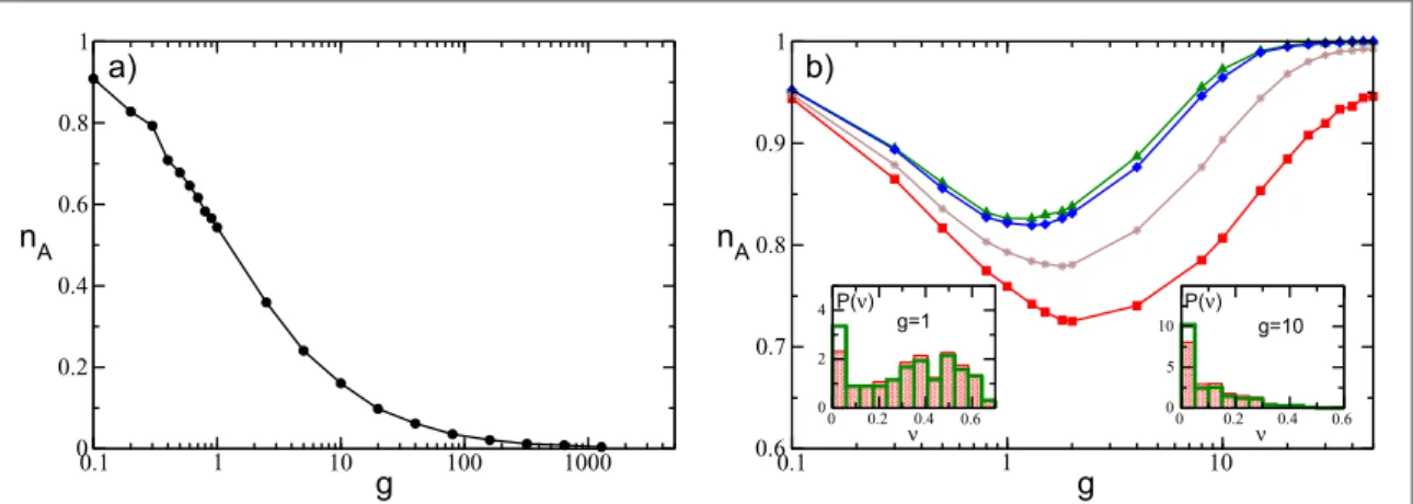
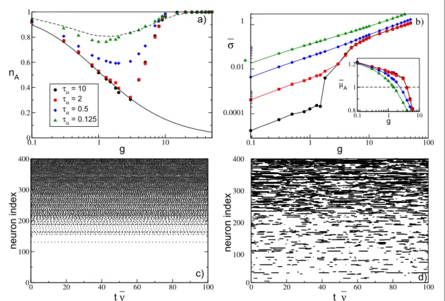
In order to exemplify the problem addressed in this paper, we report infigure1the fraction of active neurons nA(i.e. the ones emitting at least one spike during the simulation time) as a function of the strength of the

synaptic inhibition g in an heterogeneous network. For a fully coupled network, nAhas a monotonic decrease

with g(figure1(a)), while for a random sparse network, nAhas a non-monotonic behavior, displaying a

minimum at an intermediate strength gm(figure1(b)). In fully coupled networks the effect of inhibition is

simply to reduce the number of active neurons(neuronal death). However, quite counter-intuitively, in the presence of dilution by increasing the synaptic strength the previously silenced neurons can return tofiring (neuronal rebirth). Our aim is to clarify the physical mechanisms underlying neuronal death and rebirth, which are at the origin of the behavior reported in[1,66].

In particular, we consider a deterministic network of purely inhibitory pulse-coupled Leaky Integrate-and-Fire(LIF) neurons with an heterogeneous distribution of excitatory DC currents, accounting for the different level of excitability of the neurons. The evolution of this model is studied for fully coupled and for random sparse topology, as well as for synapses with different time courses. For the fully coupled case, it is possible to derive, within a self-consistent meanfield approach, the analytic expressions for the fraction of active neurons and for the averagefiring frequencyn¯as a function of coupling strength g. In this case, the monotonic decrease of nA

Figure 1. Fraction of active neurons nAas a function of the inhibitory synaptic strength g for(a) a globally coupled system, where

=

-K N 1, and(b) a randomly connected (sparse) network with K=20. In (a),the asymptotic value nAcalculated after a time

= ´

tS 1 106is reported. Conversely in(b), nAis reported at successive times: namely, tS= 985 (red squares),tS=1.1´104(brown

stars), = ´tS 5 105(blue diamonds), andtS= ´1 106(green triangles). An estimation of the times needed to reach nA= 1 can be

obtained by employing equation(13); these values range from = ´ts 5 109for g= 0.1, to ´5 105for g=50. Insets in (b) depict the probability distributionsP( )n of the single neuronfiring rate ν for the sparse network for a given g at two different times: tS= 985 (red

filled histograms) andtS= ´1 106(thick empty green histograms). The histograms are calculated by considering only active

neurons. The reported data refer to instantaneous synapses, to a system size N=400, and to an uniform distribution P(I) with =

with g can be interpreted as a Winner Takes All(WTA) mechanism [16,21,88], where only the most excitable

neurons survive the inhibition increase. For random sparse networks, neuronal rebirth can be interpreted as a re-activation process induced by erraticfluctuations in synaptic currents. Within this framework it is possible to semi-analytically obtain, for instantaneous synapses, a closed set of equations for nAas well as for the average

firing rate and coefficient of variation as a function of the coupling strength. In particular, the firing statistics of the network can be obtained via a meanfield approach by extending the formulation derived in [70] to account

for synaptic shot noise with constant amplitude. The introduction of afinite synaptic time scale does not modify the overall scenario provided that this is shorter than the membrane time constant. As soon as the synaptic dynamics become slower, the phenomenology of the transition is modified. Atg<g_mwe have a frozen phase where nAdoes not evolve in time on the explored time scales, since the currentfluctuations are negligible. Above

gmwe have a bursting regime, which can be related to the emergence of correlatedfluctuations induced by slow

synaptic times, as discussed in the framework of the adiabatic approach in[50,51].

The remainder of this paper is organized as follows: In section2we present the models that will be

considered in the paper as well as the methods adopted to characterize their dynamics. In section3we consider the globally coupled network where we provide analytic self-consistent expressions accounting for the fraction of active neurons and the averagefiring rate. Section4is devoted to the study of sparsely connected networks with instantaneous synapses, and to the derivation of the set of semi-analytic self-consistent equations providing nA, the averagefiring rate, and the coefficient of variation. In section5we discuss the effect of synapticfiltering

with a particular attention on slow synapses. Finally in section6, we briefly discuss the obtained results with a focus on the biological relevance of our model.

2. Model and methods

We examine the dynamical properties of a heterogeneous inhibitory sparse network made of N LIF neurons. The time evolution of the membrane potential viof the i-th neuron is ruled by the followingfirst-order ordinary

differential equation:

= -

-˙ ( ) ( ) ( ) ( )

v ti Ii v ti gE t ,i 1

whereg>0is the inhibitory synaptic strength, Iiis the neuronal excitability of the i-th neuron encompassing

both intrinsic neuronal properties and the excitatory stimuli originating from areas outside the considered neural circuit, and Ei(t) represents the synaptic current due to the recurrent interactions within the considered

network. The membrane potential viof neuron i evolves accordingly to equation(1) until it overcomes a

constant threshold q = 1, which leads to the emission of a spike(action potential) transmitted to all connected post-synaptic neurons while viis reset to its resting value vr= 0. The model in (1) is expressed in adimensional

units, this amounts to assume a membrane time constant t = 1m ; for the conversion to dimensional variables

see appendixA. The heterogeneity is introduced in the model by assigning to each neuron a different value of excitability Iidrawn from aflat distribution P(I), whose support is Î [I l l1, 2]withl1 q; therefore, all neurons

are supra-threshold.

The synaptic current Ei(t) is given by the linear superposition of all the inhibitory post-synaptic potentials

(IPSPs)h ( )t emitted at previous timest_nj<tby the pre-synaptic neurons connected to neuron i, namely

å

å

where K is the number of pre-synaptic neurons. Cijrepresents the elements of the N×N connectivity matrix

associated with an undirected random network, whose entries are 1 if there is a synaptic connection from neuron j to neuron i, and 0 otherwise. For the sparse network, we randomly select the matrix entries; however, to reduce the sources of variability in the network, we assume that the number of pre-synaptic neurons isfixed, namely å_{j i¹} Cij =KNfor each neuron i, where autaptic connections are not allowed. We have verified that the

results do not change if we randomly choose the links accordingly to an Erdös–Renyi distribution with a probability K/N. For a fully coupled network we have =K N-1.

The shape of the IPSP characterizes the type offiltering performed by the synapses on the received action potentials. We have considered two kinds of synapses: instantaneous ones, where h( )t =d( )t , and synapses

where the PSP is anα-pulse, namely

h_{( )t} =_{H t( )}a2_te-ta_{, ( )3} with H denoting the Heaviside step function. In this latter case the rise and decay time of the pulse are the same, namely ta=1 a, and therefore the pulse durationtPcan be assumed to be twice the characteristic timeta. Model equations(1) and (2) are integrated exactly in terms of the associated event driven maps for different

synapticfiltering, which correspond to Poincaré maps performed at the firing times (for details see appendixA) [53,91].

For instantaneous synapses, we have usually considered system sizes N=400 and N = 1400, and in the sparse case in-degrees20K80 and20 K600, respectively, with integration times up to

= ´

tS 1 106. For synapses with afinite decay time we have limited the analysis to N=400 and K=20, and to maximal integration timestS= ´1 105. Finite size dependencies on N are negligible with these parameter choices, as we have verified.

In order to characterize the network dynamics, we measure the fraction of active neuronsn tA( )S at time tS,

i.e. the fraction of neurons emitting at least one spike in the time interval[0,tS]. Therefore a neuron will be

considered silent if it has a frequency smaller than1 tS, and with our choices oftS=105-106, this

corresponds to neurons with frequencies smaller than10-3-10-4_{Hz by assuming a membrane time constant}

t = 10m ms as time scale. Estimation of the number of active neurons always begins after a sufficiently long

transient time has been discarded, usually corresponding to the time needed to deliver 106spikes in the network. Furthermore, for each neuron we estimate the time averaged inter-spike interval(ISI) TISI, the associated

firing frequency n =1 TISI, as well as the coefficient of variation CV, which is the ratio of the standard deviation

of the ISI distribution divided by TISI. For a regular spike train CV=0, and for a Poissonian distributed one

CV= 1, whileCV>1 is an indication of bursting activity. The indicators reported in the following to characterize network activity are ensemble averages over all active neurons, which we denote as ¯a for a generic

observable a.

To analyze the linear stability of the dynamical evolution we measure the maximal Lyapunov exponentλ, which is positive for chaotic evolution, and negative(zero) for stable (marginally stable) dynamics[4]. In

particular, by following[2,55], λ is estimated by linearizing the corresponding event driven map.

3. Fully coupled networks: WTA

In the fully coupled case we observe that the fraction of active neurons nAsaturates, after a short transient, to a

value that remains constant in time. In this case, it is possible to derive a self-consistent meanfield approach to obtain analytic expressions for the fraction of active neurons nAand for the averagefiring frequencyn¯of

neurons in the network. In a fully coupled network each neuron receives the spikes emitted by the other =

-K N 1 neurons; therefore, each neuron is essentially subject to the same effective input> μ, apart from the

finite size corrections (1 N).

The effective input current, for a neuron with an excitability I, is given by

m= - ¯I g n ,n A ( )4 wheren NA( -1)is the number of active pre-synaptic neurons assumed tofire with the same average

frequencyn¯.

In a meanfield approach, each neuron can be seen as isolated from the network and driven by the effective input currentμ. Taking into account the distribution of excitabilities P(I), one obtains the following self-consistent expression for the averagefiring frequency:

ò

where the integral is restricted only to active neurons, i.e. toIÎ { }IA values for which the logarithm is defined,

while =

ò

is the fraction of active neurons. In(5) we have used the fact that for an isolated LIF

neuron with constant excitability C, the ISI is simply given byTISI=ln[(C-vr) (C-q)][11].

An implicit expression for nAcan be obtained by estimating the neurons with effective inputm>q; in

particular, the fraction of silent neurons is given by

*

ò

where l1is the lower limit of the support of the distribution, while *l =g nn¯ A+q. By solving self-consistently

equations(5) and (6), one can obtain the analytic expression for nAandn¯for any distribution P(I).

In particular, for excitabilities distributed uniformly in the interval [l l1, 2], the expression for the average frequency equation(5) becomes

ò

while the fraction of active neurons is given by the following expression q n = -- + ¯ ( ) n l l l g 8 A 2 2 1

with the constraint that nAcannot be larger than one.

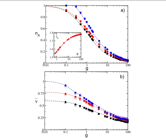
The analytic results for these quantities compare quite well with the numericalfindings estimated for different distribution intervals [l l1, 2], coupling strengths, and system sizes, as shown infigure2. For definitively large coupling g>10, some discrepancies between the mean field estimations and the simulation results are observable(see figure 2(b)). These differences are probably due to the discreteness of the pulses, which cannot be neglected for very large synaptic strengths.

As a general feature we observe that nAis steadily decreasing with g, thus indicating that a group of neurons

with higher effective inputs(winners) silence the other neurons (losers) and that the number of winners eventually vanishes for sufficiently large coupling in the limit of large system sizes. Furthermore, the average excitability of active neurons(the winners) ¯IAincreases with g, as shown in the inset offigure2(a), thus revealing

that only neurons with higher excitabilities survive the silencing action exerted by the other neurons. At the same time, as an effect of the growing inhibition, the averagefiring rate of the winners dramatically slows down. Therefore, despite the increase of¯IA, the average effective input m¯ indeed decreases for increasing inhibition.

This represents a clear example of the WTA mechanism obtained via(lateral) inhibition, which has been shown to have biological relevance for neural systems[20,60,88].

It is important to understand what is the minimal coupling value gcfor which thefiring neurons start to die.

In order to estimate gcit is sufficient to set nA= 1 in equations (7) and (8). In particular, one gets

q n

=( - ) ¯ ( )

g_c l1 , 9

Figure 2. Globally coupled systems.(a) Fraction of active neurons nAand(b) average network frequency n¯ as a function of the synaptic

strength g for uniform distributions P_{(I) with different supports. Inset: average neuronal excitability of the active neurons}¯IAversus g.

Empty(filled) symbols refer to numerical simulation with N=400 (N = 1400), and dashed lines refer to the corresponding analytic solution. Symbols and lines correspond from bottom to top to[l l1, 2]=[1.0, 1.5](black),[l l1, 2]=[1.0, 1.8](red), and

=

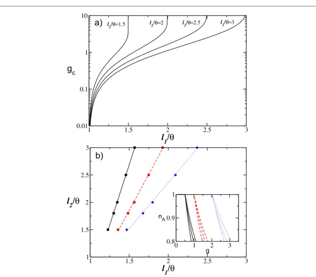
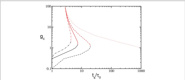
and thus, forl1=qeven an infinitesimally small coupling is in principle sufficient to silence some neurons.

Furthermore, fromfigure3(a) it is evident that whenever the excitabilities become homogeneous, i.e. for l1 l2,

the critical synaptic coupling gcdiverges toward infinity. Thus, heterogeneity in the excitability distribution is a

necessary condition in order to observe a gradual neuronal death, as shown infigure2(a).

This is in agreement with the results reported in[7], where homogeneous fully coupled networks of

inhibitory LIF neurons have been examined. In particular, forfinite systems and slow synapses, the authors in [7]

revealed the existence of a sub-critical Hopf bifurcation from a fully synchronized state to a regime characterized by oscillator death occurring at some critical gc. However, in the thermodynamic limitg_c ¥for fast as well as

slow synapses, which is in agreement with our meanfield result for instantaneous synapses.

We also proceed to investigate the isolines corresponding to the same critical gcin the(l l1, 2)-plane, and the

results are reported infigure3(b) for three selected values of gc. It is evident that the l1and l2-values associated

with the isolines display a direct proportionality among them. However, despite lying on the same gc-isoline,

different parameter values induce a completely different behavior of nAas a function of the synaptic strength, as

shown in the inset offigure3(b).

Direct simulations of the network atfinite sizes, namely for N=400 and N=1400, show that sufficiently large coupling neurons with similar excitabilities tend to form clusters, similarly to what was reported in[42], but with a

delayed pulse transmission. However, in contrast to[42], the overall macroscopic dynamics is asynchronous, and no

collective oscillations can be detected for the whole range of considered synaptic strengths.

4. Sparse networks: neuronal rebirth

In this section we will consider a network with sparse connectivity, namely each neuron is supra-threshold and it receives instantaneous IPSPs fromKNrandomly chosen neurons in the network. Due to the sparseness, the

Figure 3. Globally coupled systems.(a) Critical value gcas a function of the lower value of the excitability l1for several choices of the

upper limit l2.(b) Isolines corresponding to constant values of gcin the(l l1, 2)-plane: namely, gc= 0.5 (black solid line), gc= 1.0 (red

dashed line_{), and g}c= 2.0 (blue dotted line). Inset: Dependence of nAon g for three couples of values(l l1, 2)chosen along each of the

input spike trains can be considered as uncorrelated, and at afirst approximation it can be assumed that each spike train is Poissonian with a frequencyn¯corresponding to the averagefiring rate of the neurons in the network[8,9]. Usually, the mean activity of a LIF neural network is estimated in the context of the diffusion

approximation[69,80]. This approximation is valid whenever the arrival frequency of the IPSPs is high with

respect to thefiring emission, while the amplitude of each IPSPs (namely, =G g K) is small with respect to the

firing threshold θ. This latter hypothesis in our case is not valid for sufficiently large (small) synaptic strength g (in-degree K ), as can be appreciated by the comparison shown in figure13in appendixB. Therefore, the synaptic inputs should be treated as shot noise. In particular, here we apply an extended version of the analytic approach derived by Richardson and Swabrick in[70] to estimate the average firing rate and the average

coefficient of variation for LIF neurons with instantaneous synapses subject to inhibitory shot noise of constant amplitude(for more details see appendicesBandC).

Contrasting with the fully coupled case, the fraction of active neurons nAdoes not saturate to a constant

value for sufficiently short times. Instead, nAincreases in time due to the rebirth of losers previously silenced by

thefiring activity of winners, as shown in figure1(b). This effect is clearly illustrated by considering the

probability distributionsP( )n of thefiring rates of the neurons at successive integration times tS. These are

reported in the insets offigure1(b) for two coupling strengths and two times: namely, tS= 985 (red lines) and

= ´

tS 1 106(green lines). From these data is evident that the fraction of neurons with low firing rate (the losers) increases with time, while the fraction of highfiring neurons remains almost unchanged. Moreover, the

variation of nAslows down for increasing tS, and nAapproaches some apparently asymptotic profile for

sufficiently long integration times. Furthermore, nAhas a non-monotonic behavior with g, which is opposite to

the fully coupled case. In particular, nAreveals a minimumnAmat some intermediate synaptic strength gm

followed by an increase toward nA= 1 at large g. As we have verified, as long as <1 KN,finite size effects are

negligible and the actual value of nAdepends only on the in-degree K and the considered simulation time tS. In

the following we will try to explain the origin of such a behavior.

Despite the model being fully deterministic, due to the random connectivity the rebirth of silent neurons can be interpreted in the framework of activation processes induced by randomfluctuations. In particular, we can assume that each neuron in the network will receive n KA independent Poissonian trains of inhibitory kicks of

constant amplitude G characterized by an average frequencyn¯; thus, each synaptic input can be regarded as a single Poissonian train with total frequencyR=n KA n¯. Therefore, each neuron, characterized by its own excitability I, will be subject to an average effective inputm ( )I (as reported in equation (4)) plus fluctuations in

the synaptic current of intensity

s=g n n¯ ( )

K . 10

A

Indeed, we have verified that (10) gives a quantitatively correct estimation of the synaptic current fluctuations

over the whole range of synaptic coupling considered(as shown in figure4). A closer analysis of the probability

distributions P(IAT) of the inter-arrival times (IATs) reveals that these are essentially exponentially distributed, as expected for Poissonian processes, with a decay rate given by R, as evident fromfigure5for two different synaptic strengths. However, all these indications are not sufficient to guarantee that the IAT statistics are indeed Poissonian. In particular, as pointed out in[40], a superposition of uncorrelated spike trains generated by the

same non-Poissonian renewal process can result in a peculiar non-renewal process characterized by

exponentially distributed and uncorrelated IATs with a non-flat power spectrum. In our case we have indeed verified that for small coupling the power spectrum associated with the IATs deviates from the flat one at low frequencies, which is similar to the results reported in[40]; meanwhile, at large g the spectrum recovers a

Poissonian shape. Therefore the hypothesis that the neuronal input is Poissonian in our case should be considered only as afirst-order approximation, in particular for small synaptic couplings.

For instantaneous IPSP, the currentfluctuations are due to stable chaos [63] since the maximal Lyapunov

exponent is negative for the whole range of coupling, as we have verified. Therefore, as reported by many authors, erraticfluctuations in inhibitory neural networks with instantaneous synapses are due to finite amplitude instabilities, while at the infinitesimal level the system is stable [3,29,30,42,49,82,90].

In this circumstance, the silent neurons stay in a quiescent state corresponding to the minimum of the effective potential ( )v =v2 2-mv_{, and in order tofire they should overcome a barrier D =(q-m)}2 _2.

The average time tArequired to overcome such a barrier can be estimated accordingly to the Kramers’ theory for

activation processes[25,80], namely

t q m s - ⎛ ⎝ ⎜ ⎞ ⎠ ⎟ ( ( )) ( ) tA 0exp I , 11 2 2

wheret0is an effective time scale taking in account the intrinsic non-stationarity of the process, i.e. the fact that

It is important to stress that the expression(11) will remain valid also in the limit of large synaptic couplings,

not only because of s2_{, but also because the barrier height will increase with g. Furthermore, both these}

quantities grow quadratically with g at sufficiently large synaptic strength, as it can be inferred from equations (4)

and(10).

It is reasonable to assume that at a given time tSall neurons withtA<tSwill havefired at least once, and that

the more excitable willfire first. Therefore, by assuming that the fraction of active neurons at time tSisn tA( )S, the

last neuron that hasfired should be characterized by the following excitability:

= -

-ˆ _{( )( ) ( )}

I l2 n tA S l2 l .1 12

Here, excitabilities I are uniformly distributed in the interval [l l1, 2]. In order to obtain an explicit expression for the fraction of active neurons at time tS, one should solve the equation(11) for the neuron with excitability ˆI by

setting tS= tA, thus obtaining the following solution

f bg f fbg g = - + -< ⎧ ⎨ ⎪ ⎩ ⎪ ( ) ( ) n t n 2 4 2 if 1 1 otherwise 13 A S 2 2 A

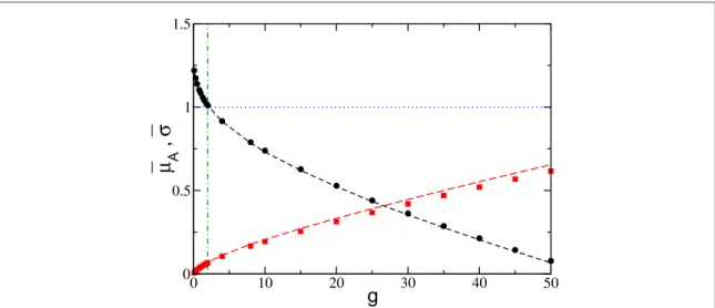
Figure 4. Effective average input of active neurons m¯A(black circles) and average fluctuations of the synaptic currentss¯(red squares)

as a function of the inhibitory coupling g. The threshold potentialq = 1is marked by the(blue) horizontal dotted line and gmby the

(green) vertical dash-dotted line. The dashed black (red) line refers to the theoretical estimation formA(σ) reported in equation (4)

(equation (10)) and averaged only over the active neurons. The data refer to N=1400, K=140,[l l1, 2]=[1.0, 1.5], and to a simulation timetS= ´1 106.

Figure 5. Probability distributions of IATs for a generic neuron in the network for(a) g = 1.3 and (b) g=10. In both panels, the red continuous line indicates the exponential distribution corresponding to a purely Poissonian process with an arrival rate given by

n

= ¯

R n KA , and the dashed blue vertical lines refer to the average IAT for the Poissonian distribution, namely1 R. The distributions

where g=(l -l)+gn f¯ = g n¯ ( t) b= -q K ln t l. 2 1 2 S 0 2

Equation(13) gives the dependence of nAon the coupling strength g for afixed integration time tSand time

scalet0whenever we can provide the value of the average frequencyn¯. A quick inspection of equations(11) and

(13) shows that, setting nA= 1, we obtain two solutions for the critical couplings gc1(gc2) below (above) that all

neurons willfire at least once in the considered time interval. The solutions are reported in figure6. In particular, we observe that wheneverl1qthe critical coupling gc1will vanish, which is analogous to the fully coupled

situation. These results clearly indicate that nAshould display a minimum for somefinite coupling strength

Î ( )

g_m g_c1,g_c2 . Furthermore, as shown infigure6the two critical couplings approach one another for increasing tSandfinally merge, indicating that at sufficiently long times all neurons will be active at any synaptic coupling

strength g.

The average frequencyn¯can be obtained analytically by following the approach described in appendixBfor LIF neurons with instantaneous synapses subject to inhibitory Poissonian spike trains. In particular, the self-consistent expression for the average frequency reads as

ò

where the explicit expression of n0is given by equation(31) in appendixB.

The simultaneous solution of equations(13) and (14) provides a theoretical estimation of nAandn¯for the

whole considered range of synaptic strength, once the unknown time scalet0isfixed. This time scale has been

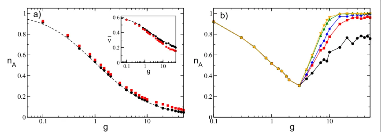
determined via an optimalfitting procedure for sparse networks with N=400 and K=20, 40, and 80 at a fixed integration timetS= ´1 106. The results for nAare reported infigure7(a). The estimated curves reproduce

reasonably well the numerical data for K=20 and 40, while for K=80 the agreement worsens at large coupling strengths. This could be due to the fact that by increasing g and K, the spike trains stimulating each neuron cannot be assumed to be completely independent, as done for the derivation of equations(13) and (14).

Nevertheless, the average frequencyn¯is quantitatively well reproduced for the considered K values over the entire range of synaptic strengths, as is evident fromfigures7(b)–(d). A more detailed comparison between the

theoretical estimations and the numerical data can be obtained by considering the distributionsP( )n of the single neuronfiring rate for different coupling strengths reported in figures7(k)–(m) for K=40. The overall

agreement can be considered as more than satisfactory, while observable discrepancies are probably due to the fact that our approach neglected a further source of disorder present in the system and related to heterogeneity in the number of active pre-synaptic neurons[9].

We have also analytically estimated the average coefficient of variation of the firing neuronsCVby extending the method derived in[70] to obtain the response of a neuron receiving synaptic shot noise input. The analytic

expressions of the coefficient of variation for LIF neurons subject to inhibitory shot noise with fixed post-synaptic amplitude are obtained by estimating the second moment of the associatedfirst-passage-time distribution; the details are reported in appendixC. The coefficient of variation can be estimated once the

self-Figure 6. Critical values gc1(black) and gc2(red) as calculated from equation (13), fixing =l2 1.5and forl1=1.2(dash-dotted),

=

l1 1.15(continuous),l1=1.1(dashed), andl1=1.0(dotted line). All values entering equation (13) are taken from simulation. All

consistent values for nAandn¯have been obtained via equations(13) and (14). The comparison with the

numerical data, reported infigures7(e)–(g), reveals a good agreement over the whole range of synaptic strengths

for all considered in-degrees.

At sufficiently small synaptic coupling the neurons fire tonically and almost independently, as shown by the raster plot infigure7(h) and by the fact thatn¯approaches the average value for the uncoupled system(namely, 0.605) andCV 0. Furthermore, the neuronalfiring rates are distributed toward finite values, indicating that the inhibition has a minor role in this case, as shown infigure7(k). By increasing the coupling, nAdecreases, and

as an effect of the inhibition more and more neurons are silenced(as evident from figure7(l)) and the average

firing rate decreases; at the same time, the dynamics become slightly more irregular, as shown in figure7(i). At

large couplingg>g_m, a new regime appears, where almost all neurons become active but with extremely slow dynamics that are essentially stochastic withCV 1, as also testified by the raster plot reported in figure7(j) and

by thefiring rate distribution shown in figure7(m).

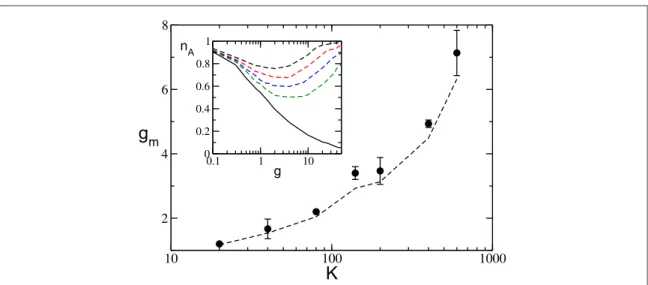
Furthermore, fromfigure7(a) it is clear that the minimum value of the fraction of active neuronsnAm decreases by increasing the network in-degree K, while gmincreases with K. This behavior is further investigated

in a larger network, namely N=1400, and reported in the inset of figure8. It is evident that nAstays close to the

globally coupled solutions over larger and larger intervals for increasing K. This can be qualitatively understood by the fact that the currentfluctuations in equation (10), responsible for the rebirth of silent neurons, are

proportional to g and scales as1 K. Therefore, at larger in-degrees thefluctuations have similar intensities only for larger synaptic coupling.

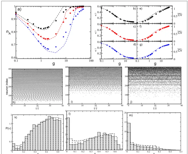
Figure 7.(a) Fraction of active neurons nAas a function of inhibition for several values of K.(b–d) Average network firing rate n¯ for the

same cases depicted in(a), and the correspondingCV(e–f). In all panels, filled symbols correspond to numerical data, and dashed

lines correspond to semi-analytic values: black circles correspond to K=20 ( t =ts 0 11), red squares to K=40 (ts t =0 19), and

blue diamonds to K=80 (ts t =0 26.6). The data are averaged over a time intervaltS= ´1 106and 10 different realizations of the

random network.(h–j) Raster plots for three different synaptic strengths for N=400 and K=40: namely, (h) =g 0.1,(i) g=1, and (j) g=8. The corresponding value for the fraction of active neurons, average frequency, and average coefficient of variation are

= ( )

nA 0.94, 0.76, 0.88, n =¯ (0.55, 0.34, 0.10 , and) CV= (0.04, 0.27, 0.76 , respectively. The neurons are ordered in terms of their) intrinsic excitability, and the time is rescaled by the average frequency n¯ ._{(k–l) Probability distributions}P( )n of the single neuron firing rate ν, for the same values of g in the panels above. Empty-discontinuous bars correspond to the theoretical prediction while filled bars indicate the histogram calculated with the simulation. The remaining parameters are as in figure1(b).

The general mechanism behind neuronal rebirth can be understood by considering the values of the effective neuronal input and currentfluctuations as a function of g. As shown in figure4, the effective input currentm¯_A, averaged over the active neurons, essentially coincides with the average excitability ¯IAforg0, where the

neurons can be considered as independent from others. The inhibition leads to a decrease ofm¯_A, and to a crossing of the thresholdθ at exactlyg=g_m. This indicates that atg<g_mthe active neurons, being on average supra-threshold,fire almost tonically inhibiting the losers via a WTA mechanism. In this case the firing neurons are essentially mean-driven and the currentfluctuations play a role in the rebirth of silent neurons only on extremely long time scales; this is confirmed by the low values of s¯ in such a range, as evident from figure4. On the other hand, forg>g_m, the active neurons are now on average below threshold whilefluctuations dominate dynamics. In particular, thefiring is now extremely irregular mainly due to re-activation processes. Therefore, the origin of the minimum in nAcan be understood as a transition from a mean-driven to afluctuation-driven

regime[68].

A quantitative definition of gmcan be given by requiring that the average input current of the active neurons m¯_Acrosses the thresholdθ atg=g_m, namely

m¯ (_g )=_I¯ -_g n_{¯ n} =q_,

A m A m m Am

where¯IAis the average excitability of thefiring neurons, whilenAmandn¯mare the fraction of active neurons and

the average frequency at the minimum.

For a uniform distribution P(I), a simpler expression for gmcan be derived, namely

n q = - ⎡ - + -⎣ ⎢ ⎤ ⎦ ⎥ ¯ ( ) ( ) g l n l l 1 2 . 15 m m1 2 A 1 2 m

We have compared the numerical measurements of gmwith the estimations obtained by employing

equation(15), wherenAmandn¯are obtained from the simulations. As shown infigure8, for a network of size

N= 1400, the overall agreement is more than satisfactory for in-degrees ranging over almost two decades (namely, for20K600). This confirms that our guess (that the minimumnAmoccurs exactly at the

transition from mean-driven tofluctuation-driven dynamics) is consistent with the numerical data for a wide range of in-degrees.

It should be stressed that, as we have verified for various system sizes (namely, N = 700, 1400, and 2800) and for a constant average in-degree K=140, for instantaneous synapses the network is in an heterogeneous asynchronous state for all considered values of synaptic coupling. This is demonstrated by the fact that the intensity of thefluctuations of average firing activity, measured by considering the low-pass filtered linear superposition of all the spikes emitted in the network, vanishes as1 N[85]. Therefore, the observed transition

atg=g_mis not associated with the emergence of irregular collective behaviors as reported for globally coupled heterogeneous inhibitory networks of LIF neurons with delay[42] or pulse-coupled phase oscillators [82].

Figure 8. gmas a function of the in-degree K. The symbols refer to numerical data, while the dashed line refers to expression(15). Inset:

nAversus g for the fully coupled case(solid black line) and for diluted networks (dashed lines); from top to bottom K=20, 40, 80, and

140. A network of size N=1400 is evolved during a period = ´tS 1 105after discarding a transient of 106spikes, and the data are averaged over 5 different random realizations of the network. Other parameters are as infigure1.

5. Effect of synaptic

filtering

In this section we will investigate how synapticfiltering can influence the previously reported results. In particular, we will consider non-instantaneous IPSP with anα-function profile(3), whose evolution is ruled by

a single time scaleta.

5.1. Fully coupled networks

Let usfirst examine the fully coupled topology. In this case we analogously observe the δ-pulse coupling by increasing the inhibition so that the number of active neurons steadily decreases toward a limit where only few neurons(or eventually only one) will survive. At the same time the average frequency also decreases

monotonically, as shown infigure9for two differenttadiffering by almost two orders of magnitude.

Furthermore, the meanfield estimations (7) and (8) obtained for nAandn¯represent a very good approximation

forα-pulses (as shown in figure9). In particular, the mean field estimation essentially coincides with the

numerical values for slow synapses, as evident from the data reported infigure9for t =a 10(black filled circles). This can be explained by the fact that for sufficiently slow synapses, with t > ¯TP ISI, the neurons feel the synaptic

input current as continuous because each input pulse has essentially no time to decay between twofiring events. Therefore, the meanfield approximation for the input current(4) works well in this case. This is particularly

true for t =a 10, where t = 20P andT¯ISI2-6in the range of the considered coupling. While for

t =a 0.125, we observe some deviation from the meanfield results (red squares in figure9). The reason for these discrepancies resides in the fact that t < ¯P TISIfor any coupling strength, and therefore the discreteness of the

pulses cannot be completely neglected, particularly for large amplitudes(large synaptic couplings). This is analogous to what is observed for instantaneous synapses.

5.2. Sparse networks

For sparse networks, nAhas the same qualitative behavior as a function of the synaptic inhibition observed for

instantaneous IPSPs, as shown infigure9(b) and figure10(a). The value of nAdecreases with g and reaches a

minimal value at gm; afterwards, it increases towards nA= 1 at larger coupling. The origin of the minimum of nA

as a function of g is the same as for instantaneous synapses. Forg<g_m, active neurons are subject to, on average, a supra-threshold effective inputm¯_Awhile at larger coupling m¯_A<q, as shown in the inset offigure10(b). This is

true for any value ofta; however, this transition from mean- tofluctuation-driven dynamics becomes dramatic for slow synapses. As evidenced from the data for the average outputfiring raten¯and the average coefficient of variationCV, these quantities have almost discontinuous jumps atg=g_m, as shown infigure11.

Therefore, let usfirst concentrate on slow synapses withtalarger than the membrane time constant, which is one for adimensional units. Forg<g_mthe fraction of active neurons is frozen in time, at least on the considered time scales, as revealed by the data infigure9(b). Furthermore, forg<g_m, the meanfield approximation obtained for the fully coupled case works almost perfectly both for nAandn¯, as reported infigure10(a). The

frozen phase is characterized by extremely small values of currentfluctuations s¯ (as shown figure10(b)) and a

quite highfiring rate n¯ 0.4-0.5 with an associated average coefficient of variationCVof almost zero(see black circles and red squares infigure11). Instead, forg>g_mthe number of active neurons increases in time

Figure 9. Fraction of active neurons nAas a function of inhibition with IPSPs withα-profiles for (a) a fully coupled topology and (b) a

sparse network with K=20. (a) Black (red) symbols correspond to t =a 10(t =a 0.125), while dashed lines are theoretical

predictions(7) and (8) previously reported for instantaneous synapses. The data are averaged over a time window = ´tS 1 105. Inset: average frequency n¯ as a function of g.(b) nAis measured at successive times: from lower to upper curves, the considered times are

= { }

tS 1000, 5000, 10000, 50000, 100000 , while t =a 10. The system size is N=400 in both cases, the distribution of excitabilities

similarly to what is observed for instantaneous synapses, while the average frequency becomes extremely small

n¯ 0.04-0.09 and the value of the coefficient of variation becomes definitely larger than one.

These effects can be explained by the fact that below gmthe active neurons(the winners) are subject to an

effective input m¯_A>qthat induces a quite regularfiring, as testified by the raster plot displayed in figure10(c).

The supra-threshold activity of the winners joined together with thefiltering action of the synapses guarantee that on average each neuron in the network receives an almost continuous current with smallfluctuations in time. These results explain why the meanfield approximation still works in the frozen phase, where fluctuations in synaptic currents are essentially negligible and unable to induce any neuronal rebirth, at least on realistic time

Figure 10._{(a) Fraction of active neurons for a network of α-pulse-coupled neurons as a function of g for various}ta: namely, t =a 10

(black circles), t =a 2(red squares),t =a 0.5(blue diamonds), and t =a 0.125(green triangles). For instantaneous synapses, the fully coupled analytic solution is reported(solid line), as well as the measured nAfor the sparse network with same level of dilution and

estimated over the same time interval(dashed line). (b) Average fluctuations of the synaptic currents¯versus g for ISPSs with α-profiles; the symbols refer to the sametaas in panel(a). Inset: Average input current m¯Aof the active neurons versus g, where the

dashed line is the threshold valueq = 1. The simulation time has beenfixed to = ´tS 1 105.(c–d) Raster plots for two different synaptic strengths for t =a 10: namely,(c) g=1 corresponds tonA0.52,n ¯ 0.45, andCV3´10-4; while(i) g=10 to



nA 0.99, n ¯ 0.06, andCV4.1. The neurons are ordered according to their intrinsic excitability and the time is rescaled by the average frequency n¯ . The data were obtained for a system size N=400 and K=20, and other parameters are as in figure9.

Figure 11.(a) Average firing rate n¯ versus g for a network of α-pulse-coupled neurons, for four values ofta. Theoretical estimations for n¯ calculated with the adiabatic approach(45) are reported as dashed lines of colors corresponding to the relative symbols. (b) Average coefficient of variationCVfor four values oftaas a function of inhibition. The dashed line refers to the values obtained for instantaneous synapses and a sparse network with the same value of dilution._{(c) Average ¯T}ISI(filled black circles) as a function of g for

t =a 10. Forg>g_mthe average inter-burst interval(empty circles) and the average ISI measured within bursts (gray circles) are also shown, together with the position of gm(green vertical line). The symbols and colors denote the sametavalues as infigure10. All the

scales. In this regime the only mechanism in action is the WTA, andfluctuations begin to have a role for slow synapses only forg>g_m. Indeed, as shown infigure10(b), the synaptic fluctuations s¯ for t =a 10(black circles) are almost negligible forg<g_mand show an enormous increase of almost two orders of magnitude at

=

g g_m. Similarly, at t =a 2(red square) a noticeable increase of s¯ is observable at the transition.

In order to better understand the abrupt changes inn¯andCVobservable for slow synapses atg=g_m, let us consider the case t =a 10. As shown infigure11(c), t >P T¯ISI2-3forg<g_m. Therefore, for these

couplings the IPSPs have no time to decay between afiring emission and the next one, and thus the synaptic fluctuations s¯ are definitely small in this case. At gman abrupt jump is observable to large values whereT¯ISI>tP,

which is due to the fact that now the neurons display bursting activities, as evident from the raster plot shown in figure10(d). The bursting is due to the fact that, forg>g_m, the active neurons are subject to an effective input, which is on average sub-threshold; therefore, the neurons tend to be silent. However, due to current

fluctuations, a neuron can pass the threshold and silent periods can be interrupted by bursting phases where the neuronfires almost regularly. In fact, the silent (inter-burst) periods are very long700-900 compared to the duration of the bursting periods, namely25-50, as shown infigure11(c). This explains the abrupt decrease

of the averagefiring rate reported in figure11(a). Furthermore, the inter-burst periods are exponentially

distributed with an associated coefficient of variation0.8-1.0, which clearly indicates the stochastic nature of the switching from the silent phase to the bursting phase. Thefiring periods within the bursting phase are instead quite regular, with an associated coefficient of variation 0.2, and with a duration similar to_T¯_ISI

measured in the frozen phase(shaded gray circles in figure11(c)). Therefore, above gmthe distribution of the ISI

exhibits a long exponential tail associated with the bursting activity, and this explains the very large values of the measured coefficient of variation. By increasing coupling, the fluctuations in the input current become larger, and thus the fraction of neurons thatfires at least once within a certain time interval increases. At the same time,

n¯, the average inter-burst periods, and thefiring periods within the bursting phase remain almost constant at

>

g 10, as shown infigure11(a). This indicates that the decrease ofm¯_Aand increase of s¯ due to the increased inhibitory coupling essentially compensate for each other in this range. Indeed, we have verified that for t =a 10 and t =a 2,m¯A(s¯) decreases (increases) linearly with g with similar slopes, namely m¯A0.88-0.029g

while s¯ 0.05+0.023 .g

For faster synapses, the frozen phase is no longer present. Furthermore, due to rebirths induced by current fluctuations, nAis always larger than the fully coupled meanfield result (8), even atg<gm. It is interesting to

notice that by decreasingta, we are now approaching the instantaneous limit, as indicated by the results reported for nAinfigure10(a) andCVinfigure11(b). In particular, for t =a 0.125(green triangles) the data

almost collapses on the corresponding values measured for instantaneous synapses in a sparse network with the same characteristics and over a similar time interval(dashed line). Furthermore, for fast synapses with t <a 1 the bursting activity is no longer present, as can be appreciated by the fact that at mostCVapproaches one in the very large coupling limit.

For sufficiently slow synapses, the average firing raten¯can be estimated by applying the so-called adiabatic approach developed by Moreno-Bote and Parga in[50,51]. This method applies to LIF neurons with a synaptic

time scale longer than the membrane time constant. In these conditions, the outputfiring rate can be

reproduced by assuming that the neuron is subject to an input current with time-correlatedfluctuations, which can be represented as colored noise with a correlation time given by the pulse duration tP=2ta(for more details see appendixD). In this case we are unable to develop a self-consistent approach to obtain at the same

time nAand the average frequency. However, once nAis provided by simulations, the estimated solution to(45)

obtained with the adiabatic approach gives very good agreement with the numerical data for sufficiently slow synapses, namely fortP1, as shown infigure11(a) for t =a 10, 2, and 0.5. The theoretical expression(45) is even able to reproduce the jump in average frequencies observable at gm, and can therefore capture the bursting

phenomenon. By considering t < 1P , as expected, the theoretical expression fails to reproduce the numerical

data, particularly at large coupling(see the dashed green line in figure11(a) corresponding to t =a 0.125). By following the arguments reported in[50], the bursting phenomenon observed for t >a 1 andg>gmcan

be interpreted at a meanfield level as the response of a sub-threshold LIF neuron subject to colored noise with correlationtP. In this case, the neuron is definitely sub-threshold, but in the presence of a large fluctuation it can

lead tofiring, and due to the finite correlation time, it can remain supra-threshold regularly firing for a period

t

_P. The validity of this interpretation is confirmed by the fact that the measured average bursting periods are of the order of the correlation time tP=2ta, namely,27-50(7-14) for t =a 10(t =a 2).

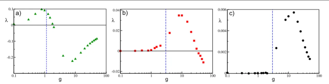
As afinal point, to better understand the dynamical origin of the measured fluctuations in this deterministic model, we have estimated the maximal Lyapunov exponentλ. As expected from previous analysis, for non-instantaneous synapses we can observe the emergence of regular chaos in purely inhibitory networks[1,30,89].

In particular, for sufficiently fast synapses, we typically note a transition from a chaotic state at low coupling to a linearly stable regime(withl < 0) at large synaptic strengths, as shown in figure12(a) for t =a 0.125. This is despite the fact that currentfluctuations are monotonically increasing with synaptic strength. Therefore,

fluctuations are due to chaos at small coupling, while at larger g they are due to finite amplitude instabilities, as expected for stable chaotic systems[3]. However, the passage from positive to negative values of the maximal

Lyapunov exponent is not related to the transition occurring at gmfrom mean-driven to afluctuation-driven

dynamics in the network.

For slow synapses,λ is essentially zero at small coupling in the frozen phase, characterized by tonic spiking of the neurons, but becomes positive by approaching gm. For larger synaptic strengthsλ, after reaching a maximal

value, it decreases and eventually becomes negative atgg_m, as reported infigures12(b)–(c). Only for

extremely slow synapses, as shown infigure12(c) for t =a 10, the chaos onset seems to coincide with the transition occurring at gm. Thesefindings are consistent with recent results concerning the emergence of

asynchronous rate chaos in homogeneous inhibitory LIF networks with deterministic[26] and stochastic [31]

evolution. However, a detailed analysis of this aspect goes beyond the scope of the present paper.

6. Discussion

In this paper we have shown that the effect reported in[1,66] is observable whenever two sources of quenched

disorder are present in the network: namely, a random distribution of neural properties and a random topology. In particular, we have shown that neuronal death due to synaptic inhibition is observable only for heterogeneous distributions of neural excitabilities. Furthermore, in a globally coupled network the less excitable neurons are silenced for increasing synaptic strength until only one or few neurons remain active. This scenario corresponds to the WTA mechanism via lateral inhibition, which has often been invoked in neuroscience to explain several brain functions[88]. WTA mechanisms have been proposed to model hippocampal CA1 activity [16], as well as

to be at the basis of visual velocity estimates[24], and to be essential for controlling visual attention [28].

However, most brain circuits are characterized by sparse connectivity[10,38,60], and in these networks we

have shown that an increase in inhibition can lead from a phase dominated by neuronal death to a regime where neuronal rebirths occur. Therefore, the growth of inhibition can have the counter-intuitive effect to activate silent neurons due to the enhancement of currentfluctuations. The reported transition is characterized by a passage from a regime dominated by the almost tonic activity of a group of neurons, to a phase where sub-thresholdfluctuations are at the origin of the irregular firing of a high number of neurons in the network. For instantaneous synapses, thefirst and second moment of the firing distributions have been obtained together with the fraction of active neurons using a meanfield approach, where the neuronal rebirth is interpreted as an activation process driven by synaptic shot noise[70].

For afinite synaptic time smaller than the characteristic membrane time constant, the scenario is similar to that observed for instantaneous synapses. However, the transition from mean-driven tofluctuation-driven dynamics becomes dramatic for sufficiently slow synapses. In this situation one observes for low synaptic strength a frozen phase, where synapticfiltering washes out the current fluctuations, thus leading to extremely regular dynamics controlled only by a WTA mechanism. As soon as the inhibition is sufficiently strong to lead the active neurons below threshold, neuronal activity becomes extremely irregular, exhibiting long silent phases interrupted by bursting events. The origin of these bursting periods can be understood in terms of the emergence of correlations in currentfluctuations induced by the slow synaptic time scale, as explained in [50].

In our model, the random dilution of network connectivity is a fundamental ingredient to generate current fluctuations, whose intensity is controlled by the average network in-degree K. A natural question is whether the reported scenario will remain observable in the thermodynamic limit. On the basis of previous studies we can affirm that this depends on how K scales with the system size [22,41,75]. In particular, if K stays finite for

 ¥

N the transition will remain observable. For K diverging with N, thefluctuations become negligible for

Figure 12. Maximal Lyapunov exponent_{λ versus g for a network of α-pulse-coupled neurons, for (a) t =}a 0.125,(b) t =a 2, and(c)

t =a 10. The blue dashed vertical line denotes the gmvalue. All the reported data were calculated for a system size N=400 and

K=20 and for simulation times5´104t 7´10

S 5, thus ensuring a good convergence ofλ to its asymptotic value. The other

sufficiently large system sizes, impeding neuronal rebirths, and the dynamics will be controlled only by the WTA mechanism.

An additional source of randomness present in the network is related to the variability in the number of active pre-synaptic neurons. In our meanfield approach we have assumed that each neuron is subject to n KA

spike trains; however, this is true only on average. The number of active pre-synaptic neurons is a random variable binomially distributed with average n KA and variancenA(1-n KA) . Future developments of the

theoretical approach reported here should include also such variability in modeling network dynamics[9].

Furthermore, we show that the considered model is not chaotic for instantaneous synapses; in such a case, we observe irregular asynchronous states due to stable chaos[63]. The system can become truly chaotic for only

finite synaptic times [3,30]. However, we report clear indications that for synapses faster than the membrane

time constanttmthe passage from mean-driven tofluctuation-driven dynamics is not related to the onset of

chaos. Only for extremely slow synapses do we have numerical evidence that the appearance of the bursting regime could be related to a passage from a zero Lyapunov exponent to a positive one. This is in agreement with the results reported in[26,31] for homogeneous inhibitory networks. These preliminary indications demand

more detailed investigations of deterministic spiking networks in order to relatefluctuation-driven regimes and chaos onsets. Moreover, we expect that it will be hard to distinguish whether the erratic currentfluctuations are due to regular chaos or stable chaos on the basis of network activity analysis, as also pointed out in[30].

Concerning the biological relevance of the presented model, we can attempt a comparison with

experimental data obtained for MSNs in the striatum. This population of neurons is fully inhibitory with sparse lateral connections(connection probability ;10%–20% [77,81]) that are unidirectional and relatively weak

[78]. Furthermore, for MSNs within the same collateral network the axonal propagation delays are quite small

;1–2 ms [76] and can be safely neglected. The dynamics of these neurons in behaving mice reveals a low average

firing rate with irregular firing activity (bursting) with an associated large coefficient of variation [47]. As we have

shown, these features can be reproduced by sparse networks of LIF neurons with sufficiently slow synapses at

>

g g_mand ta>tm. For values of the membrane time constant that are comparable to those measured for

MSNs[59,61] (namely, t  –m 10 20msec), the model is able to capture some of the main aspects of MSNs dynamics, as shown in table1. We obtain a reasonable agreement with the experiments for sufficiently slow

synapses, where the interaction among MSNs is mainly mediated by GABAAreceptors, which are characterized

by IPSP durations of the order of;5–20 ms [34,81]. However, apart the burst duration, which is definitely

shorter, all other aspects of the MSN dynamics can be already captured for ta=2tm(with t = 10m ms), as

shown in table1. Therefore, we can safely affirm, as also suggested in [66], that the fluctuation-driven regime

emerging atg>g_mis the most appropriate in order to reproduce the dynamical evolution of this population of neurons.

Other inhibitory populations are present in the basal ganglia. In particular, two coexisting inhibitory populations, arkypallidal(Arkys) and prototypical (Protos) neurons, have been recently discovered in the external globus pallidus[43]. These populations have distinct physiological and dynamical characteristics, and

have been shown to be fundamental for action suppression during the performance of behavioral tasks in rodents[44]. Protos are characterized by a high firing rate 47 Hz and a not too large coefficient of variation

(namely,CV 0.58) both in awake and slow wave sleep (SWS) states; meanwhile, Arkys have clear bursting dynamics withCV1.9[18,44]. Furthermore, the firing rate of Arkys is definitely larger in the awake state

(namely, 9 Hz) with respect to the SWS state, where firing rates are  –3 5 Hz[44].

On the basis of our results, on the one hand, Protos can be modeled as LIF neurons with reasonably fast synapses in a mean-driven regime, namely with synaptic couplingg<g_m. On the other hand, Arkys should be characterized by IPSP with definitely longer durations, and should be in a fluctuation-driven phase as suggested from the results reported infigure11. Since, as shown infigure11(a), the firing rate of inhibitory neurons

decreases by increasing synaptic strength g, we expect that the passage from awake to SWS should be

characterized by a reinforcement of Arkys synapses. Our conjectures about Arkys and Protos synaptic properties based on their dynamical behaviors ask for experimental verification, which we hope will happen shortly.

Table 1. Comparison between the results obtained for slowα-synapses and experimental data for MSNs. The numerical data refer to results obtained in the bursting phase, namely for synaptic strength g in the range [10: 50 , for simulation times] tS= ´1 105, N_{=400, and K=20. The experimental data refer to MSNs population in the striatum of free behaving wild type mice [}47_]. t ta m tm(msec) Spike rate(Hz) CV Burst duration(msec) Spike rate within bursts(Hz)

2 10 4–6 1.8 100±40 42±2

20 2–3 1.8 200±80 21±1

10 10 4–6 4.2 400±150 41±2

20 2–3 4.2 800±300 20±1